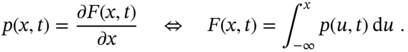
2
Probability and Stochastic Processes
In stochastic processes the future is not uniquely determined, but we have at least probability relations enabling us to make predictions.
William Feller [47], p. 420.
Signals and messages containing information about electrical, mechanical, chemical, biological, and other processes are usually affected by various types of noise and disturbances, the values of which often cannot be ignored. In such cases, the deterministic approximation becomes too rough, and probabilistic methods are used to achieve the best results. Under the influence of noise, any process becomes random, and accurate information extraction about its features requires mathematical methods describing random variables, stochastic processes, and SDEs. This chapter provides a brief introduction to the concepts and foundations of the theory of probability and stochastic processes, which will be used later in the discussion of methods of state estimation.
2.1 Random Variables
In engineering practice we often deal with some kind of experiment and elements ![]() of its random outcomes that cannot be used directly. For example, tracking distance
of its random outcomes that cannot be used directly. For example, tracking distance ![]() can be measured via time of arrival. Thus, to each
can be measured via time of arrival. Thus, to each ![]() we can assign a real number
we can assign a real number ![]() , call it random variable [191], and describe
, call it random variable [191], and describe ![]() or simply
or simply ![]() in terms of the probability theory. A collection of random variables sets up some random process.
in terms of the probability theory. A collection of random variables sets up some random process.
Scalar random variable: Since ![]() is random, it cannot be described in deterministic terms. But we may wonder how frequently the variable
is random, it cannot be described in deterministic terms. But we may wonder how frequently the variable ![]() occurs above some constant value of
occurs above some constant value of ![]() , which leads to the concept of probability. Let us think that
, which leads to the concept of probability. Let us think that ![]() occurs many times and assign an event
occurs many times and assign an event ![]() , which means that
, which means that ![]() is happening below
is happening below ![]() . The probability that
. The probability that ![]() is calculated as
is calculated as

and ![]() is represented by the cumulative distribution function (cdf),
is represented by the cumulative distribution function (cdf),
which is equal to the probability ![]() for
for ![]() to take values below
to take values below ![]() with the following properties:
with the following properties:

One might also be interested in a function that represents the concentration of ![]() values around
values around ![]() . The corresponding function
. The corresponding function ![]() is called the probability density function (pdf). But if the random variable
is called the probability density function (pdf). But if the random variable ![]() is discrete, it is represented with the probability mass function (pmf). An example is the Bernoulli distribution of two discrete random values 0 and 1.
is discrete, it is represented with the probability mass function (pmf). An example is the Bernoulli distribution of two discrete random values 0 and 1.
Both ![]() and
and ![]() are positive‐valued with the following fundamental properties:
are positive‐valued with the following fundamental properties:

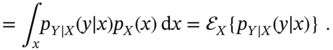
Another way to describe the properties of a random variable ![]() is to define the expectation of its exponential measure as
is to define the expectation of its exponential measure as

which is the direct Fourier transform of pdf ![]() with the variable
with the variable ![]() playing the role of negative angular frequency. The
playing the role of negative angular frequency. The ![]() function, which is usually complex, is called the characteristic function (cf) and represents
function, which is usually complex, is called the characteristic function (cf) and represents ![]() in the transform domain. Provided
in the transform domain. Provided ![]() , the pdf of
, the pdf of ![]() can be defined by inverse Fourier transform as
can be defined by inverse Fourier transform as

In some cases, one can also use the logarithm of the characteristic function or log‐characteristic function
which can be more convenient for some forms of ![]() .
.
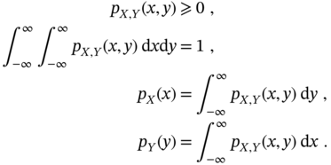
Multiple random variables: Let us now consider two random variables ![]() and
and ![]() such that, by (2.2),
such that, by (2.2), ![]() and
and ![]() . The joint cdf of
. The joint cdf of ![]() and
and ![]() is defined by
is defined by
to exist with the following main properties:

The joint pdf and cdf of random ![]() and
and ![]() relate to each other as
relate to each other as
and ![]() has the following properties:
has the following properties:
Given the distribution of a random variable ![]() , the latter can be represented in general by an infinite number of quantitative measures, called moments associated with
, the latter can be represented in general by an infinite number of quantitative measures, called moments associated with ![]() and cumulants associated with
and cumulants associated with ![]() . For example, the zero moment of
. For example, the zero moment of ![]() is its total probability (i.e., one), the first moment is the mean or average, the second central moment is the variance, the third standardized moment is the skewness, and the fourth standardized moment is the kurtosis.
is its total probability (i.e., one), the first moment is the mean or average, the second central moment is the variance, the third standardized moment is the skewness, and the fourth standardized moment is the kurtosis.
2.1.1 Moments and Cumulants
Two kinds of special characteristics called moments have found applications in the representation of random variables: raw (ordinary) moments and central moments.
Raw Moments
The raw moment of the ![]() ‐order of a random variable
‐order of a random variable ![]() is defined by the average of
is defined by the average of ![]() as
as
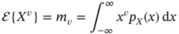
and the infinite set of raw moments completely represents the variable ![]() .
.
The ![]() ‐order raw moment of a discrete population of
‐order raw moment of a discrete population of ![]() ,
, ![]() , can be represented with the raw moments calculated by
, can be represented with the raw moments calculated by

and it represents ![]() exactly when
exactly when ![]() .
.
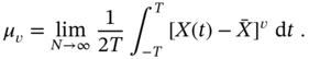
For the population of ![]() observed on a continuous time interval
observed on a continuous time interval ![]() , the raw moment can also be calculated by
, the raw moment can also be calculated by
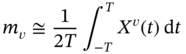
and it represents a variable ![]() exactly when
exactly when ![]() .
.
The most commonly used raw moment is of the 1‐order, ![]() , and is known as the mean or average of
, and is known as the mean or average of ![]() ,
,
There are also two other special characteristics associated with the mean of ![]() called median and mode.
called median and mode.
Median: The median “![]() ” is the value separating the higher half of the population of
” is the value separating the higher half of the population of ![]() values from the lower half. Therefore, the median may be thought as the “middle” value. For example, given a set
values from the lower half. Therefore, the median may be thought as the “middle” value. For example, given a set ![]() , the median is 5, and for
, the median is 5, and for ![]() it is 4.5. But for
it is 4.5. But for ![]() the median is also 5. Therefore, this statistic is robust against outliers.
the median is also 5. Therefore, this statistic is robust against outliers.
Mode: The “![]() ” of a population of
” of a population of ![]() is the value that appears most often. The mode is thus the value of
is the value that appears most often. The mode is thus the value of ![]() at which the pmf
at which the pmf ![]() takes its maximum value. The mode is not unique if
takes its maximum value. The mode is not unique if ![]() takes the same maximum value at several points. The most extreme case is the uniform distributions, where all values occur equally.
takes the same maximum value at several points. The most extreme case is the uniform distributions, where all values occur equally.
Mean, median, and mode: The mean, median, and mode are the same in unimodal distributions, such as the Gaussian distribution, and they are different in skewed distributions.
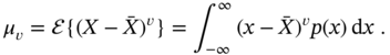
Central Moments
It is also desirable to have moments relative to the mean (2.13) of a random variable ![]() . The corresponding
. The corresponding ![]() ‐order moment
‐order moment ![]() is called the central moment and is defined by the mean value of
is called the central moment and is defined by the mean value of ![]() as
as
For discrete and continuous populations of ![]() , the
, the ![]() ‐order central moment can be determined by, respectively,
‐order central moment can be determined by, respectively,

The most common central moment has the 2‐order, ![]() , and is called the variance
, and is called the variance ![]() , which can also be calculated by
, which can also be calculated by
The root square of the variance is called the standard deviation
which always has positive values and is the degree of dissipation of a variable ![]() with respect to its mean value
with respect to its mean value ![]() .
.
Cumulants
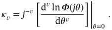
The moments of a random variable ![]() can also be determined using the expansion of cf
can also be determined using the expansion of cf ![]() in a Maclaurin series. The corresponding coefficients of the Maclaurin series are called semi‐invariants or cumulants
in a Maclaurin series. The corresponding coefficients of the Maclaurin series are called semi‐invariants or cumulants ![]() of order
of order ![]() and are calculated as
and are calculated as
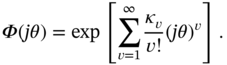
For given cumulants ![]() , the characteristic function
, the characteristic function ![]() is defined by
is defined by
It follows from the definition of ![]() that the raw moments of
that the raw moments of ![]() can be specified via
can be specified via ![]() as
as
and ![]() restored through raw moments as
restored through raw moments as

What also comes is that cumulants can be represented through moments and vise versa as ![]() ,
, ![]() ,
, ![]() , … and
, … and ![]() ,
, ![]() ,
, ![]() , …, due to exact transitions from one type of characteristics to another.
, …, due to exact transitions from one type of characteristics to another.
Skewness and Kurtosis
Symmetrically distributed ![]() is not always the case in physics and engineering, since many quantities are positive‐valued, such as distance, range, and magnitude. On the other hand, many symmetric distributions differ from the normal law by a greater rectangularity or longer tails. In such cases, two other statistics are used: skewness and kurtosis.
is not always the case in physics and engineering, since many quantities are positive‐valued, such as distance, range, and magnitude. On the other hand, many symmetric distributions differ from the normal law by a greater rectangularity or longer tails. In such cases, two other statistics are used: skewness and kurtosis.
Skewness: If a real‐valued random variable ![]() is distributed asymmetrically about the mean, skewness is often used as a measure of asymmetry. The skewness value is calculated by
is distributed asymmetrically about the mean, skewness is often used as a measure of asymmetry. The skewness value is calculated by
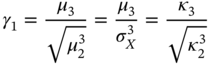
and it can be positive, negative, undefined, or zero for symmetric distributions.
Figure 2.1 illustrates the effect of skewness on a Gaussian distribution, which is unimodal and symmetric. It is seen that the mean, median, and mode are equal in the Gaussian distribution (Fig. 2.1b). However, negative skewness (Fig. 2.1a) and positive skewness (Fig. 2.1c) matter, so ![]() .
.

Figure 2.1 Effects of skewness on unimodal distributions: (a) negatively skewed, (b) normal (no skew), and (c) positively skewed.
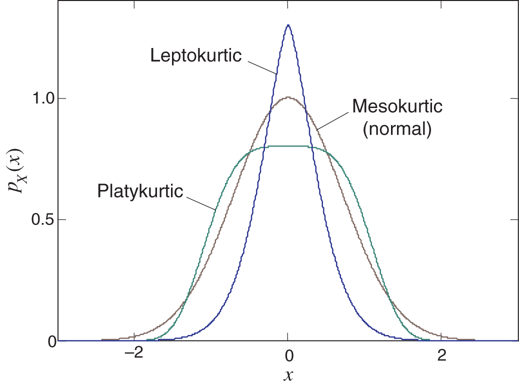
Figure 2.2 Common forms of kurtosis: mesokurtic (normal), platykurtic (higher rectangularity), and leptokurtic (longer tails).
Kurtosis: In some cases, a real‐valued random variable ![]() is distributed with multiple outliers, and kurtosis is used as a measure of the “tailedness” or “peakedness” of its pdf. In this sense, kurtosis is called a descriptor of the pdf shape. There are different ways of quantifying kurtosis and estimating it from the population of
is distributed with multiple outliers, and kurtosis is used as a measure of the “tailedness” or “peakedness” of its pdf. In this sense, kurtosis is called a descriptor of the pdf shape. There are different ways of quantifying kurtosis and estimating it from the population of ![]() . The most widely used measure of kurtosis is the fourth standardized moment
. The most widely used measure of kurtosis is the fourth standardized moment

Figure 2.2 illustrates three commonly recognized forms of kurtosis: leptocurtic, mesokurtic (normal), and platycurtic.
The difference is that the platykurtic has a higher squareness and the leptokurtic has longer tails compared to the mesokurtic, which is normal.
In Fig. 2.3 we summarize the previous analysis with connections between cdf ![]() , pdf
, pdf ![]() , cf
, cf ![]() , raw moments
, raw moments ![]() , central moments
, central moments ![]() , and cumulants
, and cumulants ![]() of a random variable
of a random variable ![]() .
.

Figure 2.3 Relationships and connections between cdf  , pdf
, pdf  , cf
, cf  , raw moments
  , central moments
  , and cumulants
  of a random variable
  .
.
2.1.2 Product Moments
Let a random variable ![]() or simply
or simply ![]() represent a random measurement
represent a random measurement ![]() and
and ![]() or
or ![]() represent a random measurement
represent a random measurement ![]() . Thus, we can think that the two variables are distributed with a joint pdf
. Thus, we can think that the two variables are distributed with a joint pdf ![]() .
.
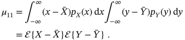
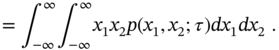
Similarly to a singe variable, the product moment ![]() of two variables
of two variables ![]() and
and ![]() is defined as follows:
is defined as follows:

Accordingly, the central product moment or the mean‐adjusted product moment is defined by

and called the covariance.
In the special case where ![]() and
and ![]() are independent, pdf
are independent, pdf ![]() is represented by the product as
is represented by the product as ![]() , and the product moments become
, and the product moments become

If two random variables ![]() and
and ![]() are independent with properties (2.28) and (2.29), then it follows that they are also uncorrelated. However, the converse is generally not true, except in a few special cases. Note also that terminologically, if
are independent with properties (2.28) and (2.29), then it follows that they are also uncorrelated. However, the converse is generally not true, except in a few special cases. Note also that terminologically, if ![]() , then the random variables
, then the random variables ![]() and
and ![]() are orthogonal.
are orthogonal.
It is often convenient to use normalized measures. The normalized mean‐adjusted product moment is called the correlation coefficient or population Pearson correlation coefficient, and it is defined as
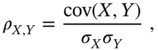
where ![]() and
and ![]() are standard deviations of variables
are standard deviations of variables ![]() and
and ![]() .
.
As the degree of correlation between two random variables ![]() and
and ![]() , the correlation coefficient ranges as
, the correlation coefficient ranges as ![]() due to the following limiting properties:
due to the following limiting properties:
- If
 , the correlation ia maximum,
  .
. - If
 , it is obvious that
  .
. - For uncorrelated
 and
and  , we have
  and hence
  .
.
Product moments are fundamental when analyzing interactions between random variables. However, if two random variables are considered at two different points in some space or at two different points in time, it is necessary to use another function, called the correlation function.
2.1.3 Vector Random Variables
Let us now represent two random variable as column vectors
where entries are drawn from populations or variables of some random processes. Such vectors can be characterized by their autocorrelation and cross‐correlation.
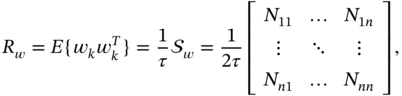
The autocorrelation matrix ![]() and autocovariance matrix
and autocovariance matrix ![]() of a vector
of a vector ![]() are defined as
are defined as


where ![]() is the variance of
is the variance of ![]() and
and ![]() is the covariance of
is the covariance of ![]() and
and ![]() for
for ![]() . It follows that matrices
. It follows that matrices ![]() and
and ![]() are square and symmetric. It can also be shown that for any vector
are square and symmetric. It can also be shown that for any vector ![]() the following values are nonnegative,
the following values are nonnegative,

and both ![]() and
and ![]() are thus positive semidefinite. Note that if the previous relationships are inequalities, matrices
are thus positive semidefinite. Note that if the previous relationships are inequalities, matrices ![]() and
and ![]() are called positive definite.
are called positive definite.
Similarly, the cross‐correlation matrix and cross‐covariance matrix of random vectors ![]() and
and ![]() are defined by, respectively,
are defined by, respectively,


2.1.4 Conditional Probability: Bayes' Rule
We have already mentioned that random variables can be distributed jointly. They can also be distributed conditionally, when the probability of one variable depends on another already observed. To arrive at probabilistic relations associated with such variables, turn to [47] and consider two events ![]() and
and ![]() that have a joint probability
that have a joint probability ![]() . We can now introduce the conditional probability
. We can now introduce the conditional probability ![]() of the event
of the event ![]() , assuming that
, assuming that ![]() is observed. The conditional probability
is observed. The conditional probability ![]() can be defined as
can be defined as
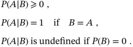
where the probability ![]() of event
of event ![]() is called marginal probability because it is independent on other events. The conditional probability
is called marginal probability because it is independent on other events. The conditional probability ![]() has the following key properties [47,91]:
has the following key properties [47,91]:
Because ![]() incorporates some already known information about the relation between two variables, it is also called an a posteriori probability, while
incorporates some already known information about the relation between two variables, it is also called an a posteriori probability, while ![]() is also called an a priori probability.
is also called an a priori probability.
By applying (2.38) to a collection of random variables ![]() , we arrive at the important chain rule
, we arrive at the important chain rule
that for three variables gives
Note that the rule (2.39) plays a fundamental role in the Bayes theory.
Bayes' Theorem
Let us consider a general case of multiple events [145]. For a finite set ![]() of mutually exclusive events called a finite partition and another event
of mutually exclusive events called a finite partition and another event ![]() such that the events
such that the events ![]() ,
, ![]() , are mutually exclusive, we can refer to the total probability theorem and write
, are mutually exclusive, we can refer to the total probability theorem and write
Using (2.38), we can further modify this relation as
because
On the other hand, since events ![]() and
and ![]() are interchangeable, we can write
are interchangeable, we can write ![]() and conclude that
and conclude that

which is stated by Bayes' theorem. Note that Tomath Bayes was the first to use conditional probability and describe the probability of an event via prior knowledge of conditions related to the event.
The conditional probability ![]() represented with (2.43) is the likelihood of event
represented with (2.43) is the likelihood of event ![]() given that event
given that event ![]() is true. Likewise,
is true. Likewise, ![]() is the likelihood of event
is the likelihood of event ![]() given that event
given that event ![]() is true. The a priori probability
is true. The a priori probability ![]() is often omitted in (2.43), and the constant
is often omitted in (2.43), and the constant ![]() is introduced (2.45) to normalize
is introduced (2.45) to normalize ![]() , to get the unit area.
, to get the unit area.
Inserting (2.41) into (2.43) gives

which generalizes Bayes' rule.
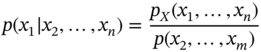
Conditional Probability Density
Considering two random variables ![]() and
and ![]() instead of two events
instead of two events ![]() and
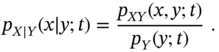
and ![]() and omitting the derivation, which can be found in [45],[145],[79], the relation (2.38) can be equivalently rewritten as
and omitting the derivation, which can be found in [45],[145],[79], the relation (2.38) can be equivalently rewritten as

where ![]() is the conditional pdf of
is the conditional pdf of ![]() given
given ![]() ,
, ![]() is the joint pdf of
is the joint pdf of ![]() and
and ![]() , and
, and ![]() is called the marginal pdf of
is called the marginal pdf of ![]() defined by
defined by

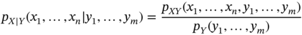
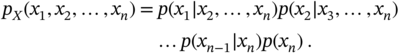
For multiple random variables collected as ![]() and
and ![]() , (2.47) can be written as
, (2.47) can be written as
and the cdf found by integrating over ![]() as
as

In the case of three random variables ![]() ,
, ![]() , and
, and ![]() , we accordingly have
, we accordingly have
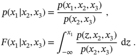
It is worth noting that the rule (2.48) allows excluding any primary variable from (2.50), and one can use (2.49) to exclude any conditional variable from (2.50). For example, given ![]() , we can find
, we can find


Most generally, for a set ![]() one can write
one can write
and, by the chain rule (2.39), obtain
2.1.5 Transformation of Random Variables
Sometimes a deterministic transformation of one random variable ![]() with known pdf
with known pdf ![]() into another
into another ![]() with unknown or desired pdf
with unknown or desired pdf ![]() is required. For example, the pdf of the system input variable
is required. For example, the pdf of the system input variable ![]() is known, and the pdf of the output variable
is known, and the pdf of the output variable ![]() must be defined. It is also often required to transform two nonlinearly related random variables into two linearly related ones, or vice versa. An example can be found in tracking where measurements made in polar coordinates are to be represented in Cartesian coordinates.
must be defined. It is also often required to transform two nonlinearly related random variables into two linearly related ones, or vice versa. An example can be found in tracking where measurements made in polar coordinates are to be represented in Cartesian coordinates.
Single‐to‐Single Variable Transformation
Let two random variables, ![]() and
and ![]() , be related to each other as follows:
, be related to each other as follows:
where ![]() and
and ![]() are some known smooth functions. Suppose we know pdf
are some known smooth functions. Suppose we know pdf ![]() for
for ![]() and would like to know pdf
and would like to know pdf ![]() for
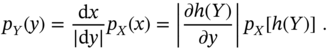
for ![]() . To find
. To find ![]() , we can refer to the dependencies of
, we can refer to the dependencies of ![]() on
on ![]() (2.56) and
(2.56) and ![]() on
on ![]() (2.57) and assert that the probability that
(2.57) and assert that the probability that ![]() lies within the interval
lies within the interval ![]() is equal to the probability that
is equal to the probability that ![]() lies within
lies within ![]() . This can be formalized as
. This can be formalized as
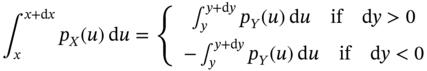
and further rewritten equivalently in the differential form as
Since we assume that ![]() , we arrive at the transformation rule
, we arrive at the transformation rule
Transformation of Vector Random Variables
Given sets of random variables, ![]() represented with pdf
represented with pdf ![]() and
and ![]() with
with ![]() . Suppose the variables
. Suppose the variables ![]() and
and ![]() ,
, ![]() , are related to each other as
, are related to each other as
Then the ![]() of
of ![]() can be defined via
can be defined via ![]() of
of ![]() as
as
where ![]() is the determinant of the Jacobian
is the determinant of the Jacobian ![]() of the transformation,
of the transformation,

2.2 Stochastic Processes
Recall that a random variable ![]() corresponds to some measurement outcome
corresponds to some measurement outcome ![]() . Since
. Since ![]() exists at some time
exists at some time ![]() as
as ![]() , the variable
, the variable ![]() is also a time function
is also a time function ![]() . The family of time functions
. The family of time functions ![]() dependent on
dependent on ![]() is called a stochastic process or a random process
is called a stochastic process or a random process ![]() , where
, where ![]() and
and ![]() are variables. As a collection of random variables, a stochastic process can be a scalar stochastic process, which is a set of random variables
are variables. As a collection of random variables, a stochastic process can be a scalar stochastic process, which is a set of random variables ![]() in some coordinate space. It can also be a vector stochastic process
in some coordinate space. It can also be a vector stochastic process ![]() , which is a collection of
, which is a collection of ![]() random variables
random variables ![]() ,
, ![]() , in some coordinate space.
, in some coordinate space.
The following forms of stochastic processes are distinguished:
- A stochastic process represented in continuous time with continuous values is called a continuous stochastic process.
- A discrete stochastic process is a process that is represented in continuous time with discrete values.
- A stochastic process represented in discrete time with continuous values is called a stochastic sequence.
- A discrete stochastic sequence is a process represented in discrete time with discrete values.
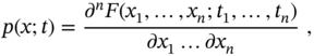
Using the concept of random variables, time‐varying cdf ![]() and pdf
and pdf ![]() of a scalar stochastic process process
of a scalar stochastic process process ![]() can be represented as
can be represented as
For a set of variables ![]() corresponding to a set of time instances
corresponding to a set of time instances ![]() , we respectively have
, we respectively have

A stochastic process can be ether stationary or nonstationary. There are the following types of stationary random processes:
- Strictly stationary, whose unconditional joint pdf does not change when shifted in time; that is, for all
 , it obeys
(2.68)
, it obeys
(2.68)
- Wide‐sense stationary, whose mean and variance do not vary with respect to time.
- Ergodic, whose probabilistic properties deduced from a single random sample are the same as for the whole process.
It follows from these definitions that a strictly stationary random process is also a wide‐sense random process, and an ergodic process is less common among other random processes. All other random processes are called nonstationary.
2.2.1 Correlation Function
The function that described the statistical correlation between random variables in some processes is called the correlation function. If the random variables represent the same quantity measured at two different points, then the correlation function is called the autocorrelation function. The correlation function of various random variables is called the cross‐correlation function.
Autocorrelation Function
The autocorrelation function of a scalar random variable ![]() measured at different time points
measured at different time points ![]() and
and ![]() is defined as
is defined as

where ![]() is a joint time‐varying pdf of
is a joint time‐varying pdf of ![]() and
and ![]() .
.
For mean‐adjusted processes, the correlation function is called an autocovariance function and is defined as

Both ![]() and
and ![]() tell us how much a variable
tell us how much a variable ![]() is coupled with its shifted version
is coupled with its shifted version ![]() .
.
There exists a simple relation between the cross‐correlation and autocorrelation functions assuming a complex random process ![]() ,
,
where ![]() is a complex conjugate of
is a complex conjugate of ![]() .
.
If the random process is stationary, its autocorrelation function does not depend on time, but depends on the time shift ![]() . For such processes,
. For such processes, ![]() is converted to
is converted to
If the joint pdf ![]() is not explicitly known and the stochastic process is supposed to be ergodic, then
is not explicitly known and the stochastic process is supposed to be ergodic, then ![]() can be computed by averaging the product of the shifted variables as
can be computed by averaging the product of the shifted variables as
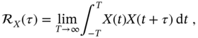
and we notice that the rule (2.73) is common to experimental measurements of correlation. Similarly to (2.73), the covariance function ![]() (2.70b) can be measured for ergodic random processes.
(2.70b) can be measured for ergodic random processes.
Cross‐Correlation Function
The correlation between two different random processes ![]() and
and ![]() is described by the cross‐correlation function. The relationship remains largely the same if we consider these variables at two different time instances and define the cross‐correlation function as
is described by the cross‐correlation function. The relationship remains largely the same if we consider these variables at two different time instances and define the cross‐correlation function as

and the cross‐covariance function as

For stationary random processes, function (2.74a) can be computed as


and function (2.75a) modified accordingly.
Properties of Correlation Function
The following key properties of the autocorrelation and cross‐correlation functions of two random processes ![]() and
and ![]() are highlighted:
are highlighted:
- The autocorrelation function is non‐negative,
 , and has the property
  .
. - The cross‐correlation function is a Hermitian function,
 .
. - The following Cauchy‐Schwartz inequality holds,
(2.77)

- For a stationary random process
 , the following properties apply:


The latter property requires the study of a random process in the frequency domain, which we will do next.
2.2.2 Power Spectral Density
Spectral analysis of random processes in the frequency domain plays the same role as correlation analysis in the time domain. As in correlation analysis, two functions are recognized in the frequency domain: power spectral density (PSD) of a random process ![]() and cross power spectral density (cross‐PSD) of two random processes
and cross power spectral density (cross‐PSD) of two random processes ![]() and
and ![]() .
.
Power Spectral Density
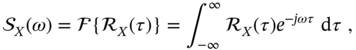
The PSD of a random process ![]() is determined by the Fourier transform of its autocorrelation function. Because the Fourier transform requires a process that exists over all time, spectral analysis is applied to stationary processes that satisfy the Dirichlet conditions [165].
is determined by the Fourier transform of its autocorrelation function. Because the Fourier transform requires a process that exists over all time, spectral analysis is applied to stationary processes that satisfy the Dirichlet conditions [165].
Dirichlet conditions: Any real‐valued periodic function can be extended into the Fourier series if, over a period, a function 1) is absolutely integrable, 2) is finite, and 3) has a finite number of discontinuities.
The Wiener‐Khinchin theorem [145] states that the autocorrelation function ![]() of a wide‐sense stationary random process
of a wide‐sense stationary random process ![]() is related to its PSD
is related to its PSD ![]() by the Fourier transform pair as
by the Fourier transform pair as

and has the following fundamental properties:
- Since
 is conjugate symmetric,
 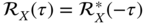 , then it follows that
  is a real function of
  of a real or complex stochastic process.
 - If
 is a real process, then
  is real and even, and
  is also real and even:
 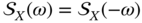 . Otherwise,
  is not even.
 - The PSD of a stationary process
 is positive valued,
  .
. - The variance
 of a scalar
  is provided by
(2.80)
is provided by
(2.80)
- Given an LTI system with a frequency response
 , then
  of an input process
  projects to
  of an output process
  as
(2.81)
as
(2.81)
Cross Power Spectral Density
Like the PSD, the cross‐PSD of two stationary random processes ![]() and
and ![]() is defined by the Fourier transform pair as
is defined by the Fourier transform pair as


and we notice that the cross‐PSD usually has complex values and differs from the PSD in the following properties:
- Since
 and
and  are not necessarily even functions of
  , then it follows that
  and
and  are not obligatorily real functions.
 - Due to the Hermitian property
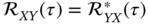 , functions
  and
and  are complex conjugate of each other,
  , and the sum of
  and
and  is real.
If ![]() is the sum of two stationary random processes
is the sum of two stationary random processes ![]() and
and ![]() , then the autocorrelation function
, then the autocorrelation function ![]() can be found as
can be found as
Therefore, the PSD of ![]() is generally given by
is generally given by
A useful normalized measure of the cross‐PSD of two stationary processes ![]() and
and ![]() is the coherence
is the coherence ![]() defined as
defined as
which plays the role of the correlation coefficient (2.30) in the frequency domain. Maximum coherence is achieved when two processes are equal, and therefore ![]() . On the other extreme, when two processes are uncorrelated, we have
. On the other extreme, when two processes are uncorrelated, we have ![]() , and hence the coherence varies in the interval
, and hence the coherence varies in the interval ![]() .
.
2.2.3 Gaussian Processes
As a collection of Gaussian variables, a Gaussian process is a stochastic process whose variables have a multivariate normal distribution. Because every finite linear combination of Gaussian variables is normally distributed, the Gaussian process plays an important role in modeling and state estimation as a useful and relatively simple mathematical idealization. It also helps in solving applied problems, since many physical processes after passing through narrowband paths acquire the property of Gaussianity. Some nonlinear problems can also be solved using the Gaussian approach [187].
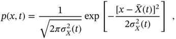
Suppose that a Gaussian process is represented with a vector ![]() of Gaussian random variables corresponding to a set of time instances
of Gaussian random variables corresponding to a set of time instances ![]() and that each variable is normally distributed with (2.37a). The pdf of this process is given by
and that each variable is normally distributed with (2.37a). The pdf of this process is given by

where ![]() ,
, ![]() , and the covariance
, and the covariance ![]() (2.34) is generally time‐varying. The standard notation of Gaussian process is
(2.34) is generally time‐varying. The standard notation of Gaussian process is
If the Gaussian process is a collection of uncorrelated random variables and, therefore, ![]() holds for
holds for ![]() and
and ![]() is diagonal, then pdf (2.85) becomes a multiple product of the densities of each of the variables,
is diagonal, then pdf (2.85) becomes a multiple product of the densities of each of the variables,

The log‐likelihood corresponding to (2.85) is
and information entropy representing the average rate at which information is produced by a Gaussian process (2.85) is given by [2]
Properties of Gaussian Processes
As a mathematical idealization of real physical processes, the Gaussian process exhibits several important properties that facilitate process analysis and state estimation. Researchers often choose to approximate data histograms with the normal law and use standard linear estimators, even if Gaussianity is clearly not observed. It is good if the errors are small. Otherwise, a more accurate approximation is required. In general, each random process requires an individual optimal estimator, unless its histogram can be approximated by the normal law to use standard solutions.
The following properties of the Gaussian process are recognized:
- In an exhaustive manner, the Gaussian process
 is determined by the mean
  and the covariance matrix
  , which is diagonal for uncorrelated Gaussian variables.
 - Since the Gaussian variables are uncorrelated, it follows that they are also independent, and since they are independent, they are uncorrelated.
- The definitions of stationarity in the strict and wide sense are equivalent for Gaussian processes.
- The conditional pdf of the jointly Gaussian stochastic processes
 and
and  is also Gaussian. This follows from Bayes' rule (2.47), according to which
- Linear transformation of a Gaussian process gives a Gaussian process; that is, the input Gaussian process
 goes through the linear system to the output as
  in order to remain a Gaussian process.
 - A linear operator can be found to convert a correlated Gaussian process to an uncorrelated Gaussian process and vice versa.
2.2.4 White Gaussian Noise
White Gaussian noise (WGN) occupies a special place among many other mathematical models of physical perturbations, As a stationary random process, WGN has the same intensity at all frequencies, and its PSD is thus constant in the frequency domain. Since the spectral intensity of any physical quantity decreases to zero with increasing frequency, it is said that WGN is an absolutely random process and as such does not exist in real life.
Continuous White Gaussian Noise
The WGN ![]() is the most widely used form of white processes. Since noise is usually associated with zero mean,
is the most widely used form of white processes. Since noise is usually associated with zero mean, ![]() , WGN is often referred to as additive WGN (AWGN), which means that it can be added to any signal without introducing a bias. Since the PSD of the scalar
, WGN is often referred to as additive WGN (AWGN), which means that it can be added to any signal without introducing a bias. Since the PSD of the scalar ![]() is constant, its autocorrelation function is delta‐shaped and commonly written as
is constant, its autocorrelation function is delta‐shaped and commonly written as
where ![]() is the Dirac delta [165] and
is the Dirac delta [165] and ![]() is some constant. It follows from (2.89) that the variance of WGN is infinite,
is some constant. It follows from (2.89) that the variance of WGN is infinite,
and the Fourier transform (2.78) applied to (2.89) gives

which means that the constant value ![]() in (2.89) has the meaning of a double‐sided PSD
in (2.89) has the meaning of a double‐sided PSD ![]() of WGN, and
of WGN, and ![]() is thus a one‐sided PSD. Due to this property, the conditional pdf
is thus a one‐sided PSD. Due to this property, the conditional pdf ![]() ,
, ![]() , of white noise is marginal,
, of white noise is marginal,
For zero mean vector WGN ![]() , the covariance is defined by
, the covariance is defined by
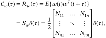
where ![]() is the PSD matrix of WGN, whose component
is the PSD matrix of WGN, whose component ![]() ,
, ![]() , is the PSD or cross‐PSD of
, is the PSD or cross‐PSD of ![]() and
and ![]() .
.
Discrete White Gaussian Noise
In discrete time index ![]() , WGN is a discrete signal
, WGN is a discrete signal ![]() , the samples of which are a sequence of uncorrelated random variables. Discrete WGN is defined as the average of the original continuous WGN
, the samples of which are a sequence of uncorrelated random variables. Discrete WGN is defined as the average of the original continuous WGN ![]() as
as

where ![]() is a proper time step.
is a proper time step.
Taking the expectation on the both sides of (2.92) gives zero,
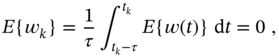
and the variance of zero mean ![]() can be found as
can be found as

where ![]() is the PSD (2.90) of WGN.
is the PSD (2.90) of WGN.
Accordingly, the pdf of a discrete WGN ![]() can be written as
can be written as
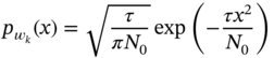
and ![]() denoted as
denoted as ![]() . Since a continuous WGN
. Since a continuous WGN ![]() can also be denoted as
can also be denoted as ![]() , the notations become equivalent when
, the notations become equivalent when ![]() .
.
For a discrete zero mean vector WGN ![]() , whose components are given by (2.92) to have variance (2.93), the covariance
, whose components are given by (2.92) to have variance (2.93), the covariance ![]() of
of ![]() is defined following (2.93) as
is defined following (2.93) as
where ![]() is the PSD matrix specified by (2.91). It follows from (2.91) and (2.94) that the covariance
is the PSD matrix specified by (2.91). It follows from (2.91) and (2.94) that the covariance ![]() of the discrete WGN evolves to the covariance
of the discrete WGN evolves to the covariance ![]() of the continuous WGN when
of the continuous WGN when ![]() as
as
Because ![]() is defined for any
is defined for any ![]() , and
, and ![]() is defined at
is defined at ![]() , then it follows that there is no direct connection between
, then it follows that there is no direct connection between ![]() and
and ![]() . Instead,
. Instead, ![]() can be viewed as a limited case of
can be viewed as a limited case of ![]() when
when ![]() .
.
2.2.5 Markov Processes
The Markov (or Markovian) process, which is also called continuous‐time Markov chain or continuous random walks, is another idealization of real physical stochastic processes. Unlike white noise, the values of which do not correlate with each other at any two different time instances, correlation in the Markov process can be observed only between two nearest neighbors.
A stochastic process ![]() is called Markov if its random variable
is called Markov if its random variable ![]() , given
, given ![]() at
at ![]() , does not depend on
, does not depend on ![]() since
since ![]() . Thus, the following is an exhaustive property of all types of Markov processes.
. Thus, the following is an exhaustive property of all types of Markov processes.
Markov process: A random process is Markovian if on any finite time interval of time instances
the conditional probability of a variable
given
depends solely on
; that is,
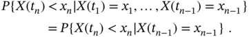
The following probabilistic statement can be made about the future behavior of a Markov process: if the present state of a Markov process at ![]() is known explicitly, then the future state at
is known explicitly, then the future state at ![]() ,
, ![]() , can be predicted without reference to any past state at
, can be predicted without reference to any past state at ![]() ,
, ![]() .
.
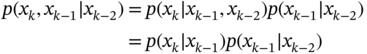
It follows from the previous definition that the multivariate pdf of a Markov process can be written as
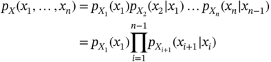
to be the chain rule (2.55) for Markov processes. In particular, for two Markovian variables one has
An important example of Markov processes is the Wiener process, known in physics as Brownian motion.
When a Markov process is represented by a set of values at discrete time instances, it is called a discrete‐time Markov chain or simply Markov chain. For a finite set of discrete variables ![]() , specified at discrete time indexes
, specified at discrete time indexes ![]() , the conditional probability (2.95) becomes
, the conditional probability (2.95) becomes

Thus, the Markov chain is a stochastic sequence of possible events that obeys (2.98). A notable example of a Markov chain is the Poisson process [156,191].
Property (2.98) can be written in pdf format as
Since (2.99) defines the distribution of ![]() via
via ![]() , the conditional pdf
, the conditional pdf ![]() for
for ![]() is called the transitional pdf of the Markov process.
is called the transitional pdf of the Markov process.
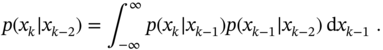
The transitional probability can be obtained for any two random variables ![]() and
and ![]() of the Markov process [79]. To show this, one can start with the rule (2.52) by rewriting it as
of the Markov process [79]. To show this, one can start with the rule (2.52) by rewriting it as
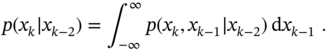
Now, according to the chain rule (2.96) and the Markov property (2.99), the integrand can be rewritten as
and (2.101) transformed to the Chapman‐Kolmogorov equation
Note that this equation also follows from the general probabilistic rule (2.53) and can be rewritten more generally for ![]() as
as

The theory of Markov processes and chains establishes a special topic in the interpretation and estimation of real physical processes for a wide class of applications. The interested reader is referred to a number of fundamental and applied investigations discussed in [16,45,79,145,156,191].
2.3 Stochastic Differential Equation
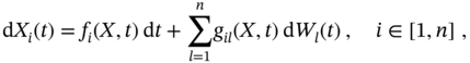
Dynamic physical processes can be both linear and nonlinear with respect to variables and perturbations. Many of them can be generalized by a multivariate differential equation in the form
where ![]() is a nonlinear function of a general vector stochastic process
is a nonlinear function of a general vector stochastic process ![]() and noise
and noise ![]() . We encounter such a case in trajectory measurements where values and disturbances in Cartesian coordinates are nonlinearly related to values measured in polar coordinates (see Example 2.5).
. We encounter such a case in trajectory measurements where values and disturbances in Cartesian coordinates are nonlinearly related to values measured in polar coordinates (see Example 2.5).
2.3.1 Standard Stochastic Differential Equation
Since noise in usually less intensive than measured values, another form of (2.104) has found more applications,
where ![]() and
and ![]() are some known nonlinear functions,
are some known nonlinear functions, ![]() is some noise, and
is some noise, and ![]() . A differential equation 2.105 or (2.106) can be thought of as SDE, because one or more its terms are random processes and the solution is also a random process. Since a typical SDE contains white noise
. A differential equation 2.105 or (2.106) can be thought of as SDE, because one or more its terms are random processes and the solution is also a random process. Since a typical SDE contains white noise ![]() calculated by the derivative of the Wiener process
calculated by the derivative of the Wiener process ![]() , we will further refer to this case.
, we will further refer to this case.
If the noise ![]() in (2.105) is white Gaussian with zero mean
in (2.105) is white Gaussian with zero mean ![]() and autocorrelation function
and autocorrelation function ![]() , and noise
, and noise ![]() in (2.106) is a Wiener process with zero mean
in (2.106) is a Wiener process with zero mean ![]() and autocorrelation function
and autocorrelation function ![]() , then (2.105) and (2.106) are called SDE if the following Lipschitz condition is satisfied.
, then (2.105) and (2.106) are called SDE if the following Lipschitz condition is satisfied.
Lipschitz condition: An equation ((2.105)) representing a scalar random process
is said to be SDE if zero mean noise
is white Gaussian with known variance and nonlinear functions
and
satisfy the Lipschitz condition
for constant
.
The problem with integrating either (2.105) or (2.106) arises because the integrand, which has white noise properties, does not satisfy the Dirichlet condition, and thus the integral does not exist in the usual sense of Riemann and Lebesgue. However, solutions can be found if we use the Itô calculus and Stratonovich calculus.
2.3.2 Itô and Stratonovich Stochastic Calculus
Integrating SDE (2.106) from ![]() to
to ![]() gives
gives
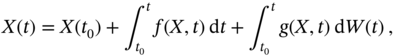
where it is required to know the initial ![]() , and the first integral must satisfy the Dirichlet condition.
, and the first integral must satisfy the Dirichlet condition.
The second integral in (2.108), called the stochastic integral, can be defined in the Lebesgue sense as [140]
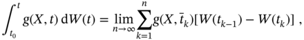
where the integration interval ![]() is divided into
is divided into ![]() subintervals as
subintervals as ![]() and
and ![]() . This calculus allows one to integrate the stochastic integral numerically if
. This calculus allows one to integrate the stochastic integral numerically if ![]() is specified properly.
is specified properly.
Itô proved that a stable solution to (2.109) can be found by assigning ![]() . The corresponding solution for (2.108) was named the Itô solution, and SDE (2.106) was called the Itô SDE [140]. Another calculus was proposed by Stratonovich [193], who suggested assigning
. The corresponding solution for (2.108) was named the Itô solution, and SDE (2.106) was called the Itô SDE [140]. Another calculus was proposed by Stratonovich [193], who suggested assigning ![]() at the midpoint of the interval. To distinguish the difference from Itô SDE, the Stratonovich SDE is often written as
at the midpoint of the interval. To distinguish the difference from Itô SDE, the Stratonovich SDE is often written as
with a circle in the last term. The circle is also introduced into the stochastic integral as ![]() to indicate that the calculus (2.109) is in the Stratonovich sense. The analysis of Stratonovich's solution is more complicated, but Stratonovich's SDE can always be converted to Itô's SDE using a simple transformation rule [193]. Moreover,
to indicate that the calculus (2.109) is in the Stratonovich sense. The analysis of Stratonovich's solution is more complicated, but Stratonovich's SDE can always be converted to Itô's SDE using a simple transformation rule [193]. Moreover, ![]() makes both solutions equivalent.
makes both solutions equivalent.
2.3.3 Diffusion Process Interpretation
Based on the rules of Itô and Stratonovich, the theory of SDE has been developed in great detail [16,45,125,145,156]. It has been shown that if the stochastic process ![]() is represented with (2.105) or (2.106), then it is a Markovian process [45]. Moreover, the process described using (2.105) or (2.106) belongs to the class of diffusion processes, which are described using the drift
is represented with (2.105) or (2.106), then it is a Markovian process [45]. Moreover, the process described using (2.105) or (2.106) belongs to the class of diffusion processes, which are described using the drift ![]() and diffusion
and diffusion ![]() coefficients [193] defined as
coefficients [193] defined as
and associated with the first and second moments of the stochastic process ![]() . Depending on the choice of
. Depending on the choice of ![]() in (2.109), the drift and diffusion coefficients can be defined in different senses. In the Stratonovich sense, the drift and diffusion coefficients become
in (2.109), the drift and diffusion coefficients can be defined in different senses. In the Stratonovich sense, the drift and diffusion coefficients become
In the Itô sense, the second term vanishes on the right‐hand side of (2.113).
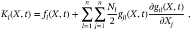
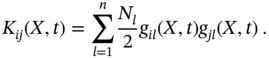
In a more general case of a vector stochastic process ![]() , represented by a set of random subprocesses
, represented by a set of random subprocesses ![]() , the
, the ![]() th stochastic process
th stochastic process ![]() can be described using SDE [193]
can be described using SDE [193]
where the nonlinear functions ![]() and
and ![]() satisfy the Lipschitz condition (2.107) and
satisfy the Lipschitz condition (2.107) and ![]() ,
, ![]() , are independent Wiener processes with zero mean
, are independent Wiener processes with zero mean ![]() and autocorrelation function
and autocorrelation function
where ![]() ,
, ![]() is the Kronecker symbol, and
is the Kronecker symbol, and ![]() is the PSD of
is the PSD of ![]() .
.
Similarly to the scalar case, the vector stochastic process ![]() , described by an SDE (2.110), can be represented in the Stratonovich sense with the following drift coefficient
, described by an SDE (2.110), can be represented in the Stratonovich sense with the following drift coefficient ![]() and diffusion coefficient
and diffusion coefficient ![]() [193],
[193],
Given the drift and diffusion coefficients, SDE can be replaced by a probabilistic differential equation for the time‐varying pdf ![]() of
of ![]() . This equation is most often called the Fokker‐Planck‐Kolmogorov (FPK) equation, but it can also be found in the works of Einstein and Smoluchowski.
. This equation is most often called the Fokker‐Planck‐Kolmogorov (FPK) equation, but it can also be found in the works of Einstein and Smoluchowski.
2.3.4 Fokker‐Planck‐Kolmogorov Equation
If the SDE (2.105) obeys the Lipschitz condition, then it can be replaced by the following FPK equation representing the dynamics of ![]() in probabilistic terms as
in probabilistic terms as
This equation is also known as the first or forward Kolmogorov equation. Closed‐form solutions of the partial differential equation (2.118) have been found so far for a few simple cases. However, the stationary case, assuming ![]() with
with ![]() , reduces it to a time‐invariant probability flux
, reduces it to a time‐invariant probability flux
which is equal to zero at all range points. Hence, the steady‐state pdf ![]() can be defined as
can be defined as

by integrating (2.119) from some point ![]() to
to ![]() with the normalizing constant
with the normalizing constant ![]() . By virtue of this, in many cases, a closed‐form solution is not required for (2.118), because pdf
. By virtue of this, in many cases, a closed‐form solution is not required for (2.118), because pdf ![]() (2.120) contains all the statistical information about stochastic process
(2.120) contains all the statistical information about stochastic process ![]() at
at ![]() .
.
The FPK equation 2.118 describes the forward dynamics of the stochastic process ![]() in probabilistic terms. But if it is necessary to study the inverse dynamics, one can use the second or backward Kolmogorov equation
in probabilistic terms. But if it is necessary to study the inverse dynamics, one can use the second or backward Kolmogorov equation
specifically to learn the initial distribution of ![]() at
at ![]() , provided that the distribution at
, provided that the distribution at ![]() is already known.
is already known.
2.3.5 Langevin Equation
A linear first‐order SDE is known in physics as the Langevin equation, the physical nature of which can be found in Brownian motion. It also represents the first‐order electric circuit driven by white noise ![]() . Although the Langevin equation is the simplest in the family of SDEs, it allows one to study the key properties of stochastic dynamics and plays a fundamental role in the theory of stochastic processes.
. Although the Langevin equation is the simplest in the family of SDEs, it allows one to study the key properties of stochastic dynamics and plays a fundamental role in the theory of stochastic processes.
The Langevin equation can be written as
where ![]() is a constant and
is a constant and ![]() is white Gaussian noise with zero mean,
is white Gaussian noise with zero mean, ![]() , and the autocorrelation function
, and the autocorrelation function ![]() . If we assume that the stochastic process
. If we assume that the stochastic process ![]() starts at time
starts at time ![]() as
as ![]() , then the solution to (2.122) can be written as
, then the solution to (2.122) can be written as

which has the mean
and the variance
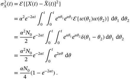
Since the Langevin equation is linear and the driving noise ![]() is white Gaussian, it follows that
is white Gaussian, it follows that ![]() is also Gaussian with a nonstationary pdf
is also Gaussian with a nonstationary pdf
where the mean ![]() is given by (2.124) and the variance
is given by (2.124) and the variance ![]() by (2.125).
by (2.125).
The drift coefficient (2.113) and diffusion coefficient (2.114) are defined for the Langevin equation 2.122 as

and hence the FPK equation 2.118 becomes

whose solution is a nonstationary Gaussian pdf (2.126) and the moments (2.124) and (2.125).
Langevin's equation is a nice illustration of how a stochastic process can be investigated in terms of a probability distribution, rather than by solving its SDE. Unfortunately, most high‐order stochastic processes cannot be explored in this way due to the complexity, and the best way is to go into the state space and use state estimators, which we will discuss in the next chapter.
2.4 Summary
In this chapter we have presented the basics of probability and stochastic processes, which are essential to understand the theory of state estimation. Probability theory and methods developed for stochastic processes play a fundamental role in understanding the features of physical processes driven and corrupted by noise. They also enable the formulation of feature extraction requirements from noise processes and the development of optimal and robust estimators.
A random variable ![]() of a physical process can be related to the corresponding measured element
of a physical process can be related to the corresponding measured element ![]() in a linear or nonlinear manner. A collection of random variables is a random process. The probability
in a linear or nonlinear manner. A collection of random variables is a random process. The probability ![]() that
that ![]() will occur below some constant
will occur below some constant ![]() (event
(event ![]() ) is calculated as the ratio of possible outcomes favoring event
) is calculated as the ratio of possible outcomes favoring event ![]() to total possible outcomes. The corresponding function
to total possible outcomes. The corresponding function ![]() is called cdf. In turn, pdf
is called cdf. In turn, pdf ![]() represents the concentration of
represents the concentration of ![]() values around
values around ![]() and is equal to the derivative of
and is equal to the derivative of ![]() with respect to
with respect to ![]() , since cdf is the integral measure of pdf.
, since cdf is the integral measure of pdf.
Each random process can be represented by a set of initial and central moments. The Gaussian process is the only one that is represented by a first‐order raw moment (mean) and a second‐order central moment (variance). Product moments represent the power of interaction between two different random variables ![]() and
and ![]() . The normalized measure of interaction is called the correlation coefficient, which is in the ranges
. The normalized measure of interaction is called the correlation coefficient, which is in the ranges ![]() . A stochastic process is associated with continuous time and stochastic sequence with discrete time.
. A stochastic process is associated with continuous time and stochastic sequence with discrete time.
The conditional probability ![]() of the event
of the event ![]() means that the event
means that the event ![]() is observed. Therefore, it is also called the a posteriori probability, and
is observed. Therefore, it is also called the a posteriori probability, and ![]() and
and ![]() are called the a priori probabilities. Bayes' theorem states that the joint probability
are called the a priori probabilities. Bayes' theorem states that the joint probability ![]() can be represented as
can be represented as ![]() , and there is always a certain rule for converting two correlated random variables into two uncorrelated random variables and vice versa.
, and there is always a certain rule for converting two correlated random variables into two uncorrelated random variables and vice versa.
The autocorrelation function establishes the degree of interaction between the values of a variable measured at two different time points, while the cross‐correlation establishes the degree of interaction between the values of two different variables. According to the Wiener‐Khinchin theorem, PSD and correlation function are related to each other by the Fourier transform.
Continuous white Gaussian noise has infinite variance, while its discrete counterpart has finite variance. A stochastic process is called Markov if its random variable ![]() , for a given
, for a given ![]() at
at ![]() , does not depend on
, does not depend on ![]() , since
, since ![]() .
.
The SDE can be solved either in the Itô sense or in the Stratonovich sense. It can also be viewed as a diffusion process and represented by the probabilistic FPK equation. The Langevin equation is a classical example of first‐order stochastic processes associated with Brownian motion.
2.5 Problems
- Two events
 and
and  are mutually exclusive. Can they be uncorrelated and independent?
 - Two nodes
 and
and  transmit the same message over the wireless network to a central station, which can only process the previously received one. Assuming a random delay in message delivery, what is the probability that 10 consecutive messages will belong to node
  ?
? - A network of 20 nodes contains 5 damaged ones. If we choose three nodes at random, what is the probability that at least one of these nodes is defective?
- Show that if
 , then 1)
  and 2)
  .
. - The binomial coefficients are computed by
 . Show that 1)
  and 2)
  .
. - Given events
 ,
,  , and
, and  and using the chain rule, show that
- Given two independent identically distributed random variables
 and
and  with zero mean, variance
  , and join pdf
  , find the pdf of the following variables: 1)
  , 2)
, 2)  , and 3)
  .
. - The Bernoulli distribution of the discrete random variable
 is given by pmf
to represent random binary time delays in communication channels. Find the cdf for (2.128) and show that the mean is
 and the variance is
  .
. - A generalized normal distribution of a random variable
 is given by the pdf
where all are real,
 is location,
  is scale, and
  is shape. Find the moments and cumulants of (2.129). Prove that the mean is
  and the variance is
  . Find the values of
  at which this distribution becomes Gaussian, almost rectangular, and heavy‐tailed.
 - The random variable
 representing the measurement noise has a Laplace distribution with pdf
where
 is the location parameter and
  is the scale parameter. Find cdf, the mean
  , and the variance
  of this variable.
 - Consider a set of
 independent samples
  ,
,  , each of which obeys the Laplace distribution (2.130) with variance
  . The maximum likelihood estimate of location is given by [13]
(2.131)
. The maximum likelihood estimate of location is given by [13]
(2.131)
and is called the median estimate. Redefine this estimate considering
 as a state variable and explain the meaning of the estimate.
 - A measured random quantity
 has a Cauchy distribution with pdf
where
 is the location parameter and
  is the scale parameter. Prove that cdf is
  and that the mean and variance are not definable.
 - Consider a measurable random variable
 represented by a Cauchy pdf (2.132) with
  and
and  . The set of measured variables passes through an electric circuit, where it is saturated by the power supply as
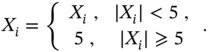
Modify the Cauchy pdf (2.132) for saturated
 and numerically compute the mean and variance.
 - The measurement of some scalar constant quantity is corrupted by the Gauss‐Markov noise
 , where
  and
and  is the white Gaussian driving noise. Find the autocorrelation function and PSD of noise
  . Describe the properties of
  in two extreme cases:
  and
and  .
. - Given a discrete‐time random process
 , where
  and
and  is some random driving force. Considering
  as input and
  as output, find the input‐to‐output transfer function
  .
. - Explain the physical nature of the skewness
 and kurtosis
  and how these measures help to recognize the properties of a random variable
  . Illustrate the analysis based on the Bernoulli, Gaussian, and generalized normal distributions and provide some practical examples.
 - The joint pdf of
 and
and  is given by
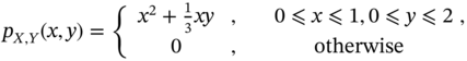
Prove that the marginal pdfs are
 and
and  .
. - Two uncorrelated phase differences
 and
and  are distributed with the conditional von Mises circular normal pdf
(2.133)
are distributed with the conditional von Mises circular normal pdf
(2.133)
where
 is a random phase mod
  and
and  is its deterministic constituent,
  is a modified Bessel function of the first kind and zeroth order, and
  is a parameter sensitive to the power signal‐to‐noise ratio (SNR)
  . Show that the phase difference
  with different SNRs
  is conditionally distributed by(2.134)
and define the function
 for
for  .
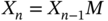
. - A stable system with random components is represented in discrete‐time state space with the state equation
 and the observation equation
  . Considering
  as input and
  as output, find the input‐to‐output transfer function
  .
. - The Markov chain
 with three states is specified using the transition matrix

Represent this chain as
 , specify the transition matrix
  , and find
  .
. - Given a stationary process
 with derivative
  , show that for a given time
  the random variables
  and
and  are orthogonal and uncorrelated.
 - The continuous‐time three‐state clock model is represented by SDE
 , where the zero mean noise
 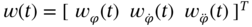 has the following components:
  is the phase noise,
  is the frequency noise, and
 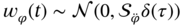 is the linear frequency drift noise. Show that the noise covariance for this model is given by
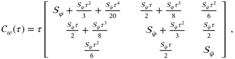
if we provide the integration from
 to
to  .
. - Two discrete random stationary processes
 and
and  have autocorrelation functions
(2.135)
have autocorrelation functions
(2.135)
which are measured relative to each point on the horizon
 by shifting
  and
and  by
by  . What is the PSD of the first process
  and the second process
  ?
? - Given an LTI system with the impulse response
 , where
  ,
,  , and
, and  is the unit step function. In this system, the input is a stationary random process
  with the autocorrelation function
  applied at
  and disconnected at
  . Find the mean
  and the mean square value
  of the output signal
  and plot these functions.
