
10
Latency Minimization Through Optimal Data Placement in Fog Networks
Ning Wangand Jie Wu
Department of Computer Science, Rowan University, Glassboro, NJ, USA
Center for Networked Computing, Temple University, Philadelphia, PA, USA
10.1 Introduction
With the wide availability of smart devices, people are able to access social websites, videos, and software from the Internet anywhere at any time. According to [1], in 2016, Netflix had more than 65 million users, with a total of 100 million hours spent streaming movies and TV shows daily. This accounted for 32.25% of the total downstream traffic during peak periods in North America. Facebook had 2.19 billion monthly active users up to the first quarter of 2018 [2]. The traditional mechanism is to store content into the central server, which leads to a relatively long data retrieving latency. To alleviate this issue, Fog Networks (FNs) are proposed and applied in commercial companies. According to Cisco's white paper [3], global streaming traffic is expected to account for 32% of all consumer traffic on the Internet by 2021, and more than 70% of this traffic will cross FNs up, an increase from 56% in 2016.
To solve the problem of the long content retrieving latency when storing data in the center, FNs can geographically store partial or entire data at fog servers deployed close to clients. This will then reduce network and center server loading times and provide a better quality of service, i.e. low latency to end-clients [4, 5]. Due to the relatively large storage space and bandwidth needs of retrieving data, an FN typically employs a limited number of fog servers, each of which has medium or low storage capacity. Such servers can collectively store a larger number of objects and serve clients from all networks with larger aggregate bandwidth needs.
An illustration of the FN network model is shown in Figure 10.1. There are five fog server nodes where data can be stored to support two different data requests, represented by red and blue colors. Note that there is a capacity limit for each server node. In a given time period, we can assume that there are different sets of data requests that arrive based on the prediction. If the data request cannot be satisfied in the local server node, it will search the nearby servers in FNs to find the requested data and there is a corresponding access latency. For example, user u2 needs to retrieve data from the server p2, which incurs a transmission from p2 to p1. The access latency between a pair of nodes is assumed to be constant over a relatively long period. In addition, there may be multiple identical data requests, for instance, trending news. In Figure 10.1, users u1 and u4 request the same data and users u2 and u3 request another data. The bandwidth and server processing speed are assumed to be sufficient, and thus, multiple identical data requests can retrieve data from the same server node.

Figure 10.1 An illustration of a typical fog network.
In this chapter, we address the latency minimization problem in FNs through data placement optimization with limited total placement budget, called the multiple data placement with budget problem (MDBP). It is motivated by the fact that the data deployment cost is the major cost in FNs [6]. However, MDBP is nontrivial. For example, in Figure 10.1, only servers p2, p3, and p4 have available storage and the available slots are 2, 1, and 1. The total budget is 3 and all link latencies are 1. The first challenge is due to the network topology. For example, it is easy to see that p5 is a bad placement location since it is far from all users. However, p2 is a good location for user u1, but bad for user u4. Therefore, for each data placement, we need to jointly consider its influence to all corresponding requests. The competition between two data requests further complicates this challenge. The second challenge is due to limited budget and request demands. In this example, users u1 and u4 have relatively larger demands; these high demand users should have low access latency but it does not mean that we need to always assign them more data copies. For example, it may be the case all the high demand requests are close to each other. The third challenge is due to copy distribution. If we have multiple data for a request, its decision should be further revised. For example, if we use two data copies for data request 1, we can place data at locations p2 and p4 to satisfy users u1 and u4 so that they both have low access latency. In addition, the limited storage size of each server location further complicates the proposed problem. It is because we cannot simply apply the individual solutions of each single data request since they may violate the server storage constraint.
We discuss the solution for the MDBP in two different cases depending on whether there is data replication. In the first case, we do not consider data replication so that we can focus on optimizing data placement. We find that we can transfer the MDBP into a min-cost flow formulation and thus find the optimal solution. We also propose a local information collection method to reduce the time complexity of the min-cost flow transformation in the tree topology, the common topology of FNs. In a general case with data replication, the MDBP turns out to be NP-complete even when there is only one type of data request. We propose a dynamic programming solution to find the optimal solution in the single request scenario with line topology. In the general case, we first propose a heuristic algorithm. However, its performance is related to the system environments. In addition, we further propose a novel assignment approach based on the rounding technique. It first finds the optimal fractional solution and then gradually transfers into the integer solution without avoiding the server capacity constraint. The proposed approach is proved to have an approximation ratio of 10.
The contributions of this chapter are summarized as follows:
- To our best knowledge, we are the first to consider the optimal data placement with budget in FNs for multiple data requests under the server capacity constraint.
- We find the optimal solution of MDBP in the scenario where there is no data replication through min-cost flow formulation, and propose a local information collection method to reduce the time complexity.
- In the general case, we prove that the MDBP is NP-complete. A novel rounding approach is proposed, and it has a constant approximation ratio of 10.
- We verify the effectiveness of the proposed approaches using the PlanetLab trace, which is a worldwide Internet trace.
The remainder of the chapter is organized as follows: the related works are in Section 10.2. The problem statement is in Section 10.3. The min-cost flow formulation is provided in Section 10.4 for the data placement without replication. In the general scenario, we first prove that the proposed problem is NP-complete and then propose a novel rounding solution with approximation analysis in Section 10.5. The experimental results from the PlanetLab trace are shown in Section 10.6, and we conclude the chapter with Section 10.7.
10.2 Related Work
The data placement problem [7, 8] in FNs is a fundamental problem. The existing work can be briefly categorized into two types based on whether the data placement changes with time.
10.2.1 Long-Term and Short-Term Placement
Early work in [9] studied the k-cache placement problem in a given network with special topologies, i.e. line and ring. The difference between [9] and this chapter is that in [9], each data can fractionally support clients, but this assumption is not true in this chapter. The work in [10] studied the trade-off between selecting a better traffic-delivery path and increasing the number of FN servers. In recent work in [6], the authors considered the dynamic network demand and found that deploying data close to the end-users might not always be the optimal solution. In [1], to find the optimal on-demand content delivery in the short term (e.g. one-week), the authors formulated and solved the content placement problem with the constraints of storage space and edge bandwidth. In [11], the authors discussed the optimal data update frequency decision in data placement. In [12], the authors provided a hierarchical data management architecture to maximize the traffic volume served from data and minimize the bandwidth cost (Table 10.1).
10.2.2 Data Replication
The work in [13] addressed the facility location problem with different client types, which is equivalent to the case of data placement without replication since there is only one facility for a type of client. Authors in [14] discuss the optimal single data request placement with replication in the tree topology. The optimal solution is obtained through the dynamic programming technique. In [15], data can be transferred between a set of proxy servers and thus the authors optimized the data transformation cost. In [16], authors jointly considered optimization of data replication costs and access latency. In [17], they jointly consider the data receiving for multiple different data. Therefore, the co-locations of data are important.
Table 10.1 Summary of symbols.
| Symbol | Interpretation |
| m | Total type of data request |
| n | Number of fog servers |
| pi | Server i |
| si | Server pi's storage size |
| lij | Access latency to between servers pi to pj |
| dij | Demand of the data request j at server i |
| xij | Server node i has data j |
| θ | Data placement budget |
| Overall data placement planning | |
| Latency of dij with a placement planning |
This chapter addresses long-term data placement with data replication. Our work differs from existing works by considering multiple data requests with different demands and limited total placement budgets.
10.3 Problem Statement
In this section, we discuss the proposed network models, followed by the problem formulation and challenges.
10.3.1 Network Model
An FN is an overlay network over the Internet; it is composed of a set of fog servers. The server nodes are potential places for data deployment. Without loss of generality, we model the topology of the overlay network with a connected undirected graph G(V, E), where V is the set of vertices denoting the servers, and E is the set of edges denoting the data transmission between servers in the network and the edge weight is the corresponding latency. We assume that the topology of the target network is known in advance and there is a total of n server nodes in the FN, i.e. ∣V ∣ = n. Note that there is a storage limit in each server, denoted by si.
This chapter considers an off-line scenario. We assume that there are m different data in total. For each data, there can be one or multiple data requests (up to n). A data request is denoted by dij, which means there is a request from location i for the data j and the value of dij is the total demand at that location. Let ![]() be a feasible placement plan. For each data request, it will be satisfied by the nearest server that stores the data in the FN. The nearest data can be found through the shortest-path algorithms. Therefore, for a data request dij, its latency for a given placement planing
be a feasible placement plan. For each data request, it will be satisfied by the nearest server that stores the data in the FN. The nearest data can be found through the shortest-path algorithms. Therefore, for a data request dij, its latency for a given placement planing ![]() is
is ![]() , which is
, which is
Currently, we assume that all data requests are the same size. In the future, we might extend it to a more general case where different data requests might have different sizes.
10.3.2 Multiple Data Placement with Budget Problem
To meet all data requests and minimize data access latency, the system provider can place data in the server nodes of FNs. However, the data placement can be costly. Therefore, we propose the MDBP to minimize the average data access latency for the FN. Specifically, the MDBP is as follows – we would like to plan the data placement locations to minimize the user's data access latency while avoiding the server's capacity. Based on whether there is replication, we consider two versions: (1) there is only one data for each data request in the network. (2) There may be multiple data for a data request, but there is an overall data placement budget. The problem can be mathematically formulated as follows.


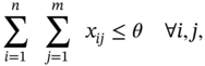
where ![]() is a placement decision. The first constraint, i.e. Equation (10.3), means that each server cannot exceed its capacity. The second constraint, i.e. Equation (10.4), is the total budget constraint where θ is the given placement budget. The last constraint, i.e. Equation (10.5), means that data cannot be partitioned.
is a placement decision. The first constraint, i.e. Equation (10.3), means that each server cannot exceed its capacity. The second constraint, i.e. Equation (10.4), is the total budget constraint where θ is the given placement budget. The last constraint, i.e. Equation (10.5), means that data cannot be partitioned.
Note that in the aforementioned formulation, the MDBP does not consider the users' mobility [17], that is, a data request represents a user. However, it can be easily extended to a case that considers users' mobility. The idea of the conversion is that we can transfer a mobile user into multiple static users in the MDBP, where the demand of each static user is the percentage of staying at that mobile node [18]. An example is shown in Figure 10.1, where there are two users. User 1 spends 60% of its time in p1, and 40% of its time in p4. User 2 spends 50% of its time in p1 and p3. After the conversion, we can apply the solution of MDBP to the extended model.
10.3.3 Challenges
The proposed MDBP is nontrivial even when the user request pattern is given/predicted, because we need to jointly consider the data placement distribution for multiple data requests. We cannot simply consider each data request individually and then combine the solutions. The reason is that it might be the case that there are optimal locations for multiple data requests, but the server storage size is not large enough to hold all of them. Given the data replication, how to jointly distribute the data in each type of request another challenge. An illustration of the challenges of the MDBP is shown in Figure 10.2, where there are two different types of data requests and three available servers. We ignore the access servers in this example. The weights on the edges represent the corresponding communication latency. In this toy example, the storage size of each of these three servers is 2, 2, and 1, respectively, and the total data budget in the network is 4. In this example, all data requests have the unit demand to simplify the illustration. We propose four different strategies to minimize the overall latency and show the placement challenge. First, if we place one data copy for data request 1 and three data copies for data request 2, we find that improper placement leads to large latency. In strategy 1, the latency for data request 1 is 7 + 2, and the latency for data request 2 is 3 + 2 + 1. Therefore, the overall latency is 15. In this toy example, strategies 1 and 2 and strategies 3 and 4 have the same data distribution but different latencies. In addition, this example shows that different data distributions influence on the latency, i.e. strategies 3 and 4 have lower latency compared to strategies 1 and 2.

Figure 10.2 An illustration of the problem's challenges.
10.4 Delay Minimization Without Replication
In this section, we focus on the storage placement optimization without replication. The problem formulation is introduced first, followed by the min-cost flow solution.
10.4.1 Problem Formulation
The MDBP can be simplified since different data have no influence on each other in terms of the latency and thus, Equation (10.1) can be reformulated as follows.


where xij is a decision variable to show that the server pi has a data j. The first constraint is that each data can be placed at one location and only one location in the network and therefore, there is no replication. The second constraint is that the total amount of data placed at a server node cannot exceed its capacity constraint.
10.4.2 Min-Cost Flow Formulation
In this subsection, we would like to explain that the MDBP can be solved by the min-cost flow formulation.
Figure 10.3 shows the min-cost flow formulation for the example in Figure 10.2. Each data request can be assigned to any server. The capacity constraint of each server location is controlled by the edge flow constraint between the server node and virtual destination in the min-cost flow formulation. For example, the cumulated latency for data request 1 in three servers is 9, 7, and 7, respectively. The min-cost flow can be solved by the successive shortest path [20].
10.4.3 Complexity Reduction
In this subsection, we design an efficient local information collecting method that can reduce the overall time complexity of cumulated latency calculation in min-cost flow calculation. The time complexity of calculating the cumulated latency of each type of data request in all server locations is O(n2) in the simple approach since we need to traverse the network for each data request. Here, we show that the overall time complexity can be reduced to O(n) in the tree topology, which is the common topology in FNs [21].
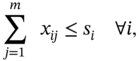
The procedure is as follows: We transfer G into a tree by considering an arbitrary node as the root node. Then, we aggregate the latency cost gradually from the leaves to the root of the networks. For each node i, it keeps a vector of Ci, Ci = {c1, c2, ⋯, ck}, where k is the total number of data requests. It records its distance to all the data request access locations. In Figure 10.4, k = 2. Initially, all elements in the vector are 0. Then, we calculate the total latency of the data placement in any node by using the following two steps:
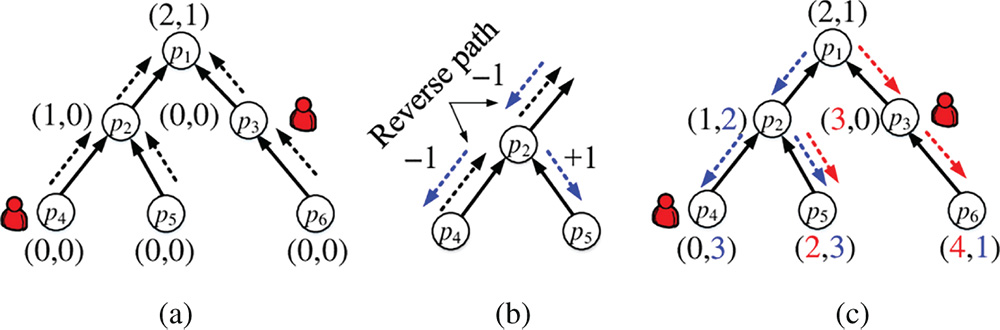
Figure 10.4 An illustration of latency updating procedure: (a) demand collection, (b) updating rule, (c) demand updating.
- Upward information collection. We gradually update the latency value of each element cj in Ci from leaf nodes to the root node as follows. If we have seen the corresponding data request from a successor node i′, then
 . Otherwise, cj keeps its original value.
 - Downward information updating. We gradually update the latency value in the revised visiting order to summarize the information from different branches. If the branch is used in the information collection and the corresponding data is seen again, then
 . Otherwise,
  .
.
After the information updating is done, the placement cost of a location is ![]() . Since the each node will be only visited twice, the overall time complexity is O(n).
. Since the each node will be only visited twice, the overall time complexity is O(n).
An illustration is shown in Figure 10.4, where all edge weights are units. Since the calculation is independent for different data requests, we use a data request to illustrate the procedure. In Figure 10.4, the data requests generate at server nodes p3 and p4. There are two data requests in this example. Each server node keeps a bracket, where each element records the distance from the current location to the corresponding data request location. Note that in the upward information collection procedure, each node only collects the distance information of the data requests in its subtree. Therefore, at the end, only the root node has the information of all data requests. In downward information updating, the information collected by the root is distributed in all branches. The data updating of the node p2 illustrates one case, where the corresponding distance decreases by 1. The data updating of the node p4 illustrates two cases: (i) 3 increases by 1 for data request 1, and (ii) 0 increases by 1 for data request 2, since the distance to data requests 1 and 2 increases. Note that here, we use a binary tree as an example, but this method works in any tree topology.
10.5 Delay Minimization with Replication
In this section, the problem hardness in the general case is discussed first, followed by the optimal solution in a line topology, and the solution in the general scenario.
10.5.1 Hardness Proof
The k-median problem is as follows: in a metric space, G(E, V), there is a set of clients C ∈ V, and a set of facilities F ∈ X. We would like to open k facilities in F, and then assign each client node j to the selected center that is closest to it. If location j is assigned to a center i, we incur a cost cij. The goal is to select k centers so as to minimize the sum of the assignment cost.
The reduction from a special case of the MDBP to the k-median problem is as follows: in a special case of the MDBP, we assume that there is only one type of data request. In this setting, there is no capacity constraint since each available server node should have at least one storage space. Assume that the total budget is k. We need to determine the data placement location, which is equivalent to finding the centers (facilities) in the k-median problem. Its weight is the total latency cost for the data request at the corresponding server location. Clearly, if we set the latency as the corresponding cij in the k-median problem, we can apply the solution of the MDBP to the k-median problem.
10.5.2 Single Request in Line Topology
We have proven that the MDBP problem is NP-complete in the general graph even in the simple request case. However, when the FN has some particular topology, i.e. the line topology, we can determine the optimal placement for that user by using dynamic programming in the single data request scenario. Specifically, we first sort all data requests directionally. Then, we can define a state called opt[i, j], which represents the minimum cost for that data request up to the first i requests with j copies. Then, we can update opt[i, j] as follows.
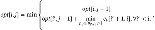
where i′ is a request prior to request i. The ck[i′ + 1, i] is the latency for assigning a new data copy at server pk, which is between ![]() and pi to cover data requests in this range. The idea behind Equation (10.10) is that the optimal solution always falls into one of two cases: (1) we have moved to the location i without adding one more data copy to get the optimal result; (2) we have moved to the location i and we can use one more data copy to reduce the overall latency.
and pi to cover data requests in this range. The idea behind Equation (10.10) is that the optimal solution always falls into one of two cases: (1) we have moved to the location i without adding one more data copy to get the optimal result; (2) we have moved to the location i and we can use one more data copy to reduce the overall latency.
A toy example can be used to illustrate the proposed dynamic programming in Figure 10.5. In this example, let us assume that θ = 2, which means that we can use two data copies at most. Initially, we can use only one data to cover three users. After calculating the four available server locations, opt[1, 1] = 0, opt[1, 2] = 3, and opt[1, 3] = 4, which achieve the optimal value when the data is put at p1, p2, and p3. Then, we add one more data copy into the network. It is easy to calculate opt[2, 1] = 0, opt[2, 2] = 0, opt[2, 3] = 1. Here is an example of a calculation of opt[2, 3].

In Equation (10.11), we use the ![]() and ignore the calculation procedure. It is clear that opt[1, 1] + c3[2, 3] = 1 is the minimum in this example.
and ignore the calculation procedure. It is clear that opt[1, 1] + c3[2, 3] = 1 is the minimum in this example.
10.5.3 Greedy Solution in Multiple Requests
If there are multiple different requests, we cannot simply apply the optimal solution for each request because it might not make a feasible solution if we add them together.
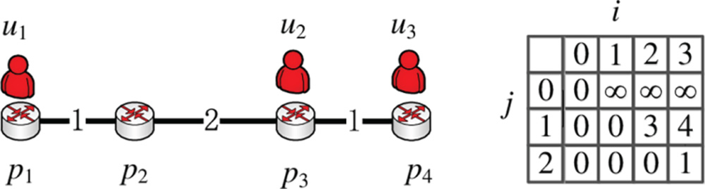
Figure 10.5 The dynamic programming in the line topology.
To address this problem, we first propose the following heuristic algorithm as shown in Algorithm 10.2. Initially, when the data request is not covered, we go through all types of data requests and calculate their optimal data placements so far. The data whose placement leads to the minimum latency in each round will be selected to put into the network. It is shown in lines 1–4. After that, there is one data for any data request in the network to ensure the coverage constraint. Then, for each round, we pick the data, which can reduce the latency maximum if that data can change its location once, shown in lines 5–8. However, the proposed heuristic may be far from optimal. An example is shown in Figure 10.6, where there is one slot fog server location 1 and 3 to store data. The greedy solution is shown in Figure 10.5. It will select the blue data request in the first round due to the smallest latency increase. However, this option leads to the large latency at the second round. The optimal solution is shown in Figure 10.5, where the placement decision jointly considers two data requests.
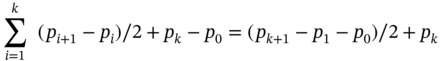

Figure 10.6 An illustration of the greedy algorithm: (a) greedy, (b) optimal.
Instead, if we assign each data request to the first server location at the left, the overall latency is
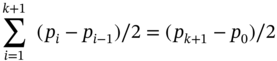
Then, ![]() when k is a large number. The number of data requests at a time also has an influence on the ratio and the ρ, which is the maximum number of requests in the network over time. Therefore, the overall approximation ratio is 3ρ.
when k is a large number. The number of data requests at a time also has an influence on the ratio and the ρ, which is the maximum number of requests in the network over time. Therefore, the overall approximation ratio is 3ρ.
According to Theorem 10.4, we know that the proposed heuristic algorithm cannot achieve good performance even in the line topology. Therefore, it is necessary to propose an approach that can guarantee adequate performance in different network environments.
10.5.4 Rounding Approach in Multiple Requests
To improve the performance of the greedy solution, we propose a two-step rounding solution. In the first step, we relax the proposed problem into the linear programming (LP) and obtain the lower bound of the MDBP. Then we propose a novel rounding technique, which first rounds a half-integral solution through the min-cost flow. Then, we can further convert the half-integral solution to an integer solution.
10.5.4.1 Generating Linear Programming Solution
The linear programming formulation of the MDBP problem is,


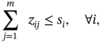

which is formulated from the angle of each data request. Therefore dk is the demand for a data request k. Let us assume that the total number of data requests is h. Note that h ≥ m due to the repeated data requests. In this formulation, yijk means the server node i has data j and covers data request k fractionally, zij means that server i has zij amount of data j. Equations (10.15, 10.16) ensure that each data request has to be satisfied and the assignment is feasible. Equation (10.17) is the capacity constraint for each server, and Equation (10.18) is the total placement budget constraint.
10.5.4.2 Creating Centers
Since it is hard to directly convert the fractional solution to integral solution, we would like to aggregate the assignment into several “center” servers, so that each center has at least a half-data. To simplify the following explanation, we create the notation ![]() , which is the unit demand cost of the LP solution for data request k. Let us consider all the data requests that need data j. We sort them in increasing order of the Ck. Then, for each data request k, if there is an another data request k′ and
, which is the unit demand cost of the LP solution for data request k. Let us consider all the data requests that need data j. We sort them in increasing order of the Ck. Then, for each data request k, if there is an another data request k′ and ![]() , we would like to consolidate the demand on data request dk to
, we would like to consolidate the demand on data request dk to ![]() , that is,
, that is, ![]() . We apply this procedure to all data requests; the remaining servers with nonzero demands are called center servers. Since each data moves at most 4Lk, it is clear that any solution can incur an additive factor of at most 4OPT (Figure 10.7).
. We apply this procedure to all data requests; the remaining servers with nonzero demands are called center servers. Since each data moves at most 4Lk, it is clear that any solution can incur an additive factor of at most 4OPT (Figure 10.7).
10.5.4.3 Converting to Integral Solution
After we get the data center servers, an important issue is how we can assign data requests so that the result is an integral solution that doesn't violate the server's capacity constraint. We refer to [22] to propose a two-phase solution where the first step is to build a half-integral solution. This ensures that the distance between a data request and the server serving it is fractionally bounded by the access cost. Therefore, the fractional solution is equivalent to a feasible flow to a min-cost flow problem with integral capacities. Note that to apply the solution in [23] to the MDBP, we need to add a virtual node before going to the destination with the link capacity as the total budget. With the property of the min-cost flow, we can always find an integer solution of no greater cost. By applying the min-cost flow transformation in [23], it has an approximation ratio of 6.
The proposed algorithm has a constant approximation ratio of 10. The center creation incurs at most 4OPT. The half-integral solution transformation introduces at most 3OPT. The integer solution conversion further leads to 2OPT. Therefore, the overall cost is 4 + 2 × 3 = 10OPT.
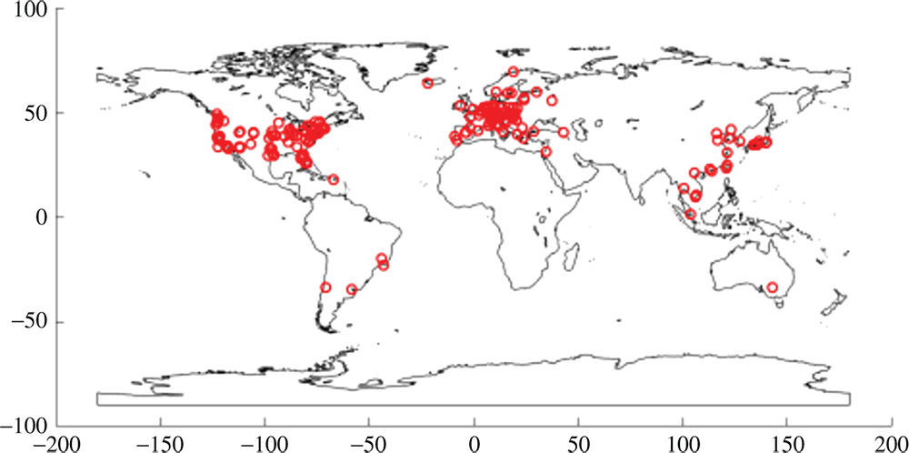
Figure 10.7 Server distribution.
10.6 Performance Evaluation
We evaluate the performance of the proposed solution in this section. The compared algorithms, the trace, the simulation settings, and the evaluation results are presented as follows.
10.6.1 Trace Information
In this chapter, we use the PlanetLab trace [24] generated from the PlanetLab testbed. PlanetLab is a global research network that supports the development of new network services. It contains a set of geo-distributed hosts running PlanetLab software worldwide. In this trace, the medians of all latencies, i.e. round trip time (RTT), between nodes are measured through the King method. 325 PlanetLab nodes and 400 other popular websites are measured (Figure 10.8).
In the PlanetLab trace, the domain of each node is provided. Each node's geometric location is retrieved through the domain-to-IP database and the IP-to-Geo database, provided by [25, 26], respectively. Some domains are no longer in service. In the end, there are 689 nodes. It is reported that the mapping error is within 5 mi and can be ignored in our experiments. Figure 10.9 shows the trace visualization results.
10.6.2 Experimental Setting
We conduct experiments on two scales, i.e. the world and the United States. At the United States scale, we use the nodes on the west coast to simulate the line-topology. The number of data requests, m, changes from 2 to 5. The number of users changes from 10 to 20, which are randomly selected from the first 325 nodes in the PlanetLab trace. The data request location is randomly generated in each round. The pair latency is known and therefore, the topology is not important in the experiments. The number of data placement budgets also changes in the experiments from m to 2m. We change the following four settings in the experiments: (1) the number of data budgets, (2) the number of data, (3) the number of the data requests, and (4) different server capacities.

Figure 10.8 Latency-distance mapping: (a) greedy, (b) optimal.

Figure 10.9 Performance comparison without data replication.
10.6.3 Algorithm Comparison
We compare five algorithms in the experiments:
- Random (RD) algorithm. It is a benchmark algorithm. During the first m rounds, a type i data is randomly selected and placed. After that, a data is randomly selected and put into the network.
- Min-volume (MV) algorithm. The data whose placement leads to the minimal cost increase is selected. Specifically, in the first m rounds, if a data has been selected, it cannot be selected again.
- Iteration updating (IU) algorithm. The IU algorithm places different data requests in an order so that the location that leads to the minimal cost increase is selected in each round.
- Min-cost (MC) algorithm. The MC algorithm is proposed in this chapter and it is explained in Section 10.4 when there is no data replication.
- Rounding (RO) algorithm. The RO algorithm is proposed in this chapter and it is explained in Section 10.5.4.
In a special scenario without data replication, the IU algorithm doesn't work since each data always has one data copy, and is thus removed in this case. Besides, the RD algorithm is not necessary since the MC algorithm is optimal.
10.6.4 Experimental Results
10.6.4.1 Trace Analysis
We verify the access latency between servers and their corresponding distances. The mapping result is shown in Figure 10.10. We use three different distance measurement methods, that is, the shortest path, which is the geodistance of the corresponding GPS coordinates, the sum of latitude and longitude distances, and the area between two nodes in terms of latency estimation. Figure 10.9 shows the cumulative distribution functions of three distance measurements, i.e. Figure 10.9 shows that using the shortest path has a relatively low estimation error, i.e. 10% for 80% of nodes when using the shortest path to estimate the latency between a pair of servers.
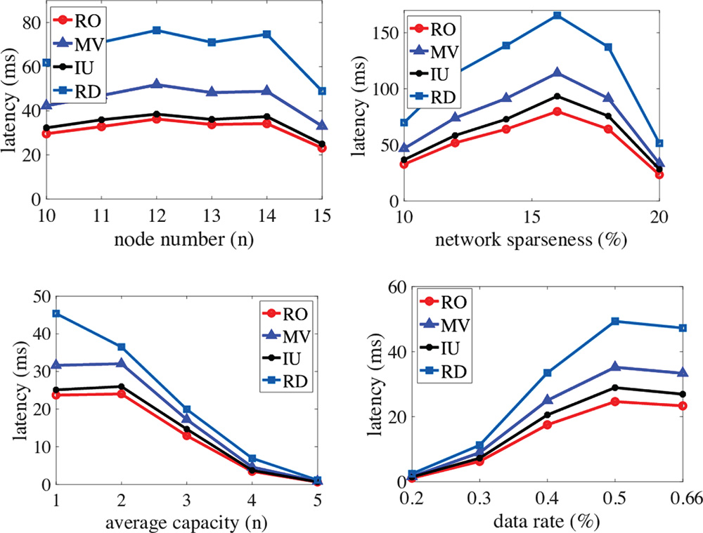
Figure 10.10 Performance comparison with data replication.
10.6.4.2 Results Without Data Replication
Figure 10.9 shows the results of the performance of proposed algorithms in the case, where there is no data replication. The results clearly show that the proposed MC algorithm achieves the lowest latency, followed by the MV algorithm. The RD algorithm's performance is the worst, which demonstrates the necessity of data placement optimization. In Figure 10.9, we change the number of servers in the experiments, i.e. the size of the FNs. The result shows that when the FNs have a larger size, improper data placement leads to bad performance. The RD algorithm has more than 100% of the MC algorithm's latency in Figure 10.9. In Figure 10.9, we gradually increase the average number of edges in the network with a certain amount of servers. The results show that when the network is sparse, there is a large performance difference between algorithms. In the experiments, the average latency decreases around 20% with a lower network spareness level. The IU algorithm has similar performance to MV since they are both greedy algorithms that cannot generate the optimal data placement order.
In Figure 10.9, we change the average storage size of each server. The results show that the average latency is relatively stable. A possible reason is that the data is generated uniformly in the experiments and thus, the placement of data into different locations has minimum influence on the final result. Figure 10.9 shows the results of different data request rates. When the data request rate increases, all algorithms have a larger latencies.
10.6.4.3 Results with Data Replication
Figure 10.10 shows the performance of proposed algorithms in a case where there is data replication. The budget number is two times the number of data request in the experiments. The results clearly show that the proposed RO algorithm achieves the lowest latency, followed by the IU, MV, and RD algorithms. The RD algorithm's performance is the worst, which demonstrates the necessity of data placement optimization.
In Figure 10.10, we change the number of servers in the experiments, i.e. the size of the FNs. The results show that when the FNs have a larger size, improper data placement leads to bad performance. The RD algorithm has more than 150% the latency of the IU algorithm in Figure 10.10. Compared with the results in Figure 10.9, all algorithms have better performance due to a greater amount of data placed in the network. In Figure 10.10, we gradually increase the average number of edges in the network with a certain amount of servers. The results show that when the network is sparse, the performance difference between different algorithms is large. An interesting result is that the average latency first increases, then later decreases with an increase in the network sparseness level.
In Figure 10.10, we change the average storage size of each server. The results show that along with an increase in average storage size, the latency decreases very quickly due to increased placement flexibility. In Figure 10.9, the average latency is reduced by more than 20% with one additional storage capacity in the server node. Figure 10.10 shows the results of different data request rates. When the data request rate increases, all algorithms have a larger latency. However, the RD algorithm has the fastest speed in terms of latency increasing, which demonstrates the effectiveness of the data placement optimization.
10.6.4.4 Summary
Based on the experiments, we find that data placement optimization is very necessary. The average performance can be improved by more than 50% in most cases by comparing the proposed algorithms with the random placement. In a general case with data replication, the proposed RO algorithm has significant improvement compared to other algorithms, which indicates that both the data budget distributions in each data request and their corresponding placements are very important.
10.7 Conclusion
In this chapter, we consider the data placement issue in the FNs so that users have low access delay. Specifically, we discuss the MDBP, whose objective is to minimize the overall access latency. We begin with a simple case, where there is no data replication. In this case, we propose a min-cost flow transformation and thus find the optimal solution. We further propose efficient updating strategy to reduce the time complexity in the tree topology. In a general case with data replication, we prove that the proposed problem is NP-complete. Then, we propose a novel rounding algorithm, which incurs a constant-factor increase in the solution cost. We validate the proposed algorithm by using the PlanetLab trace and the results show that the proposed algorithms improve the performance significantly.
Acknowledgement
This research was supported in part by NSF grants CNS 1824440, CNS 1828363, CNS 1757533, CNS 1629746, CNS-1651947, CNS 1564128.
References
- 1 Gomez-Uribe, C.A. and Hunt, N. (2016). The Netflix recommender system: algorithms, business value, and innovation. ACM Transactions on Management Information Systems 6 (4): 13.
- 2 Statistica, Facebook statistics, 2018 [Online]. Available: https://www.statista.com/statistics/264810/number-of-monthly-active-facebook-users-worldwide
- 3 Cisco Visual Networking Index: Forecast and methodology, 2016–2021 [Online]. Available: https://www.cisco.com/c/en/us/solutions/collateral/service-provider/global-cloud-index-gci/white-paper-c11-738085.html
- 4 Ghose, D. and Kim, H.J. (2000). Scheduling video streams in video- on-demand systems: a survey. Multimedia Tools and Applications 11 (2): 167–195.
- 5 Claeys, M., Bouten, N., De Vleeschauwer, D. et al. (2015). An announcement-based caching approach for video-on-demand streaming. In: Proceedings of the 2015 11th International Conference on Network and Service Management (CNSM). IEEE, November 9–13.
- 6 Tang, G., Wu, K., and Brunner, R. (2017). Rethinking CDN design with distributee time-varying traffic demands. In: Proceedings of the IEEE INFOCOM. IEEE, May 1–4.
- 7 Sahoo, J., Salahuddin, M.A., Glitho, R. et al. (2016). A survey on replica server placement algorithms for content delivery networks. IEEE Communications Surveys & Tutorials 19 (2): 1002–1026.
- 8 N. Wang and J. Wu, Minimizing the subscription aggregation cost in the content-based pub/sub system, in Proceedings of the 25th International Conference on Computer Communications and Networking (ICCCN), 2016.
- 9 Krishnan, P., Raz, D., and Shavitt, Y. (2000). The cache location problem. IEEE/ACM Transactions on Networking 8 (5): 568–582.
- 10 M. Yu, W. Jiang, H. Li, and I. Stoica, Tradeoffs in CDN designs for throughput oriented traffic, in Proceedings of the 8th International Conference on Emerging Networking Experiments and Technologies (CoNEXT '12), ACM, December 10–13, 2012.
- 11 Applegate, D., Archer, A., Gopalakrishnan, V. et al. (2010). Optimal content placement for a large-scale vod system. IEEE/ACM Transactions on Networking 24 (4, ACM): 2114–2127.
- 12 S. Borst, V. Gupta, and A. Walid, Distributed caching algorithms for content distribution networks, in Proceedings of the 29th Conference on Information Communications (INFOCOM '10), IEEE, San Diego, CA, March 14–19, 2010.
- 13 Wang, L., Li, R., and Huang, J. (2011). Facility location problem with different type of clients. Intelligent Information Management 3 (03): 71.
- 14 B. Li, M. J. Golin, G. F. Italiano, X. Deng, and K. Sohraby, On the optimal placement of web proxies in the Internet, in Proceedings of the IEEE INFOCOM '99, IEEE, March 21–25, 1999.
- 15 Xu, J., Li, B., and Lee, D.L. (2002). Placement problems for transparent data replication proxy services. IEEE Journal on Selected Areas in Communications 20 (7): 1383–1398.
- 16 Hu, M., Luo, J., Wang, Y., and Veeravalli, B. (2014). Practical resource provisioning and caching with dynamic resilience for cloud-based content distribution networks. IEEE Transactions on Parallel and Distributed Systems 25 (8): 2169–2179.
- 17 K. A. Kumar, A. Deshpande, and S. Khuller, Data placement and replica selection for improving co-location in distributed environments, arXiv preprint arXiv:1302.4168, 2013.
- 18 Tärneberg, W., Mehta, A., Wadbro, E. et al. (2017). Dynamic application placement in the mobile cloud network. Future Generation Computer Systems 70: 163–177.
- 19 L. R. Ford Jr and D. R. Fulkerson, A simple algorithm for finding maximal network flows and an application to the Hitchcock problem, Technical Report, 1955.
- 20 A. Goldberg and R. Tarjan, Solving minimum-cost flow problems by successive approximation, in Proceedings of the ACM STOC, 1987.
- 21 L. Gao, H. Ling, X. Fan, J. Chen, Q. Yin, and L. Wang, A popularity-driven video discovery scheme for the centralized P2P-VoD system, in Proceedings of the WCSP 2016, Yangzhou, China, IEEE, 2016.
- 22 M. Charikar, S. Guha, É. Tardos, and D. B. Shmoys, A constant-factor approximation algorithm for the k-median problem, in Proceedings of the Thirty-first Annual ACM Symposium on Theory of Computing (SOTC '99), Atlanta, GA, May 1–4, 1999.
- 23 Baev, I., Rajaraman, R., and Swamy, C. (2008). Approximation algorithms for data placement problems. SIAM Journal on Computing 38 (4): 1411–1429.
- 24 C. Lumezanu and N. Spring, Measurement manipulation and space selection in network coordinates,in Proceedings of the 28th International Conference on Distributed Computing Systems (ICDCS 2008), IEEE, Beijing, China, June 17–20, 2008.
- 25 InfoByIP, Domain and IP bulk lookup tool [Online]. Available: https://www.infobyip.com/ipbulklookup.php.
- 26 Maxmind [Online]. Available: www.maxmind.com.