14.1 Introduction

Internet of Things (IoT) has gained remarkable and rapid development today and has been widely adopted into industry and daily life [1]. Human-facing and machine-to-machine applications are coming into being, where end-to-end latency are both well worth mentioning. The human-facing applications, such as gaming, virtual reality [2], and multimedia services [3], are needed to guarantee the quality of service (QoS) and quality of experience (QoE) to optimize the user experience and satisfaction. Meanwhile, for the machine-to-machine applications, such as motion control in cars, the requests need to be timely responsive [4]. IoT systems are expected to meet the latency requirements with finite resources to support these real-time applications and to optimize the latency has become a major problem for IoT responsive applications.

Fog computing [5] has been developed to decrease the latency of IoT applications since it is realized near the IoT devices and the data sources. It mainly consists of the basic computation model and the data transmission model to collect, process, and send data accordingly and reduce the data transmission volume over the Internet. In that case, the latency of applications as well as the battery power consumed to send and receive data are decreased, respectively. Meanwhile, the user experience is improved. It is said that responsive IoT applications are considered to be one of the primary reasons for the adoption of fog computing [2]. However, to fully exploit the computing system structure and solve the resource scheduling problem is not a trivial task as the fog computing infrastructure is complex. In addition, different requirements developed by users brings difficulties to model the problem. It's known that the task scheduling on multiprocessors problem is NP-hard when two processors are used [6]. This problem focuses on the latency optimization for responsive IoT applications under the fog computing environment. This problem, which considers more factors, can also be proved to be NP-hard, so there is no known polynomial algorithm for this problem until now.

The remainder of the chapter is organized as follows: Section 14.2 outlines estimation of distribution algorithm (EDA) and its application in the area of scheduling. Section 14.3 reviews the related work about fog computing system and methods to model and reduce the latency of applications. Section 14.4 provides the problem statement including system model, application model, time-dependent utility functions and objectives in mathematic formulas.

And in Section 14.5, we elaborate our proposed algorithm, including decoding and encoding method, EDA scheme and the local search procedure. The simulation environment parameters, comparison algorithms are introduced in Section 14.6 and in Section 14.6.1 the comparison results are given. In the end, we conclude our paper in Section 14.7 with some conclusions and future work.

14.2 Estimation of Distribution Algorithm

The evolutionary optimization algorithms have been proven to be very efficient to solve NP-hard optimization problems in the past two decades. The evolutionary optimization algorithms are good at solving the nonconvex, discrete optimization problems to achieve acceptable solutions in limited time. EDA was a kind of efficient population-based evolutionary algorithm. Statistic theory and methods are the most important part of EDA. A certain probability model is built according to the problem information in EDA and it's adopted to be sampled and produced the population. Meanwhile, the probability model is updated by the elite individuals in the population. Thus, the evolution of EDA is driven by updating the probability model. The basic procedure of EDA is:

1. Initialize the population and the probability model;
2. Sample the probability model randomly to achieve new population and replace the formal population with the new one;
3. Choose the elite solutions in accordance to the objective function;
4. Update the probability value of the model with the elite individuals by certain statistic learning method;
5. If the stopping criterion is met, output the best solution until now; or, turn to step 2.

According to the different types of selection operator for selecting elite solutions, the class of probability models, and the updating procedure of the probability model, EDAs could be divided into different types. Some classical probability models, such as the univariate model, chain model, bayesian network and tree model, have been applied to solve different kinds of problems, such as machine learning [7], bioinformatics [8], and production scheduling problems [9].

For the complex scheduling problems, the EDA scheme embedded with a knowledge-driven local search method performs well as the proposed algorithm and is good at both exploration and exploitation. In our previous work, our proposed EDA performed well in a direct acyclic graph (DAG) scheduling problem for both cloud computing [10] and fog computing infrastructure [11, 12]. The application completion time, the total tardiness of application, energy consumption of cloud or fog computation nodes and the lifetime of IoT system have been considered as the optimization objectives and well optimized in our previous work. Inspired by the successful application of EDA for this problem, the uEDA in this work will be adopted to maximize the task utility to optimize the task scheduling and computation resource allocation.

14.3 Related Work

As IoT has been realized initially and fog computing is put forward, lots of new research focused on the related topics is proposed. The measurement, modeling, and optimization of end-to-end latency of IoT applications are discussed. A detailed introduction to the fog computing and related algorithms is offered in [13]. Resource management, cooperative offloading, and load balancing are all needed to consider the fog computing environment. QoS is considered to be one of the important objectives for the algorithms enabling real-time applications. In [2], the authors examine the properties of task latencies in fog computing by considering both traditional and wireless fog computing execution points. Similarly, the authors consider the fog computing service assignment problem in bus networks [14]. A model minimizing the communication costs and maximizing utility with tolerance time constraints is given to formulate the problem.

To model the latency and optimize the task scheduling, many metrics are developed. Tardiness is a well-known metric to measure how much a task is delayed. Total tardiness, weighted total tardiness, the largest tardiness value and the number of delayed tasks are all designed to measure whether a batch of tasks is processed on time and how much they're delayed. Surveys such as [15, 16] offer total tardiness problems. They mainly introduce the single machine problem as well as the parallel machine and flowshop problem. In [17], the authors survey the weighted and unweighted tardiness problems. On the other hand, the task utility is an efficient performance measure for the real-time systems [18]. Different kinds of time-dependent functions are tailored for tasks with different response time needs. To distinguish the hard and soft deadline constrained tasks, we prefer time-dependent functions to measure the performance of scheduling algorithm rather than weighted total tardiness. In this way, there is no need to ensure the weighted parameter value.

14.4 Problem Statement

A generalized three-tier IoT system [19] is shown in Figure 14.1. This system consists of things, fog, and cloud tiers.

IoT devices, such as sensors and cameras, are deployed to collect data and process it accordingly. To fully cover the corresponding region, each cluster consists of heterogeneous IoT devices and is located into different places. As the different clusters are far away from each other, there is no directed transmission between the clusters and within the same cluster, IoT devices are assumed to be fully connected.

The fog computing tier is located near the IoT devices to reduce the data transmission. Different devices, such as a laptop, Raspberry Pi, and local servers are defined as fog nodes. Each fog node is in charge of a cluster of IoT devices and preprocess and send the computation tasks for the further computation. Within the fog tier, the devices are fully connected.

The cloud tier is the third tier of the system, which is usually far away from the IoT data sources. The containers with computation and storage capabilities are considered as cloud nodes. The cloud nodes are considered more reliable and efficient than things and fog nodes. In our model, the fog tier is connected with the cloud tier and within the cloud tier, the processors are fully connected with each other.

For the IoT applications, it is represented as a DAG because most applications can be modeled as workflow. We use the nodes in DAG to model the computation tasks while the edges to model the precedence constraints. The weight value on the edge represents the data size transferred between the tasks. The communication-to-computation ratio (CCR) is calculated as average communication time divided by computation time and is used to describe the application.

To measure the QoE for each task, the utility-related information of each task to reduce the latency of each task and accelerate the completion of the application, to maximize the sum of task utility is adopted as the objective of this work. The utility task j is calculated as follows in this work:

(14.1)

where time-dependent utility function [18] f_j(t) represents the utility of task j on certain completion time point C_j. According to different needs, different functions are used to describe the requirements on the tasks. In this work, two kinds of tasks are considered. Some tasks must be finished before a certain deadline, such as for the motion control, otherwise it will lead to serious results. For these tasks, they are considered as hard deadline constrained and the step function, shown as (14.2), is used as their utility function. In addition, some tasks are soft deadline constrained and the wait-readily-first function is used, shown as (14.3).

(14.2)

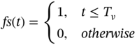
where T_v denotes the hard deadline of the certain task. This function implies that if the task is finished before T_v, its utility is settled as 1, otherwise, the utility turns to be 0.

(14.3)

where T_e, T_s denotes soft deadline interval of a certain task. If the task is finished before T_e, its utility equals 1, and after T_e, the utility decreases as the finish time increases. If it's finished after T_s, the utility turns to be 0. In this way, the objective of this problem is designed as:

(14.4)

In this work, both hard deadline and soft deadline constrained tasks are given two deadline values (d1j, d2j). For the hard deadline constrained tasks, d1j = d2j = Tvj is settled. And for the soft deadline constrained tasks, we have d1j = Tej, d2j = Tsj. The deadline value information is given in advance.

Because of the precedence constraints, all the tasks can only start being processed after all its input data from its parent tasks are received. And the tasks are nonpreemptive during processing. The communication time between any two connected tasks (i, j) is dependent on the transmission rate B(m_i, m_j) associated with the assigned computing nodes(m_i, m_j), (m_i ≠ m_j). Thus, the earliest start time of task j (EST_j) could be indicated as follows:

(14.5)

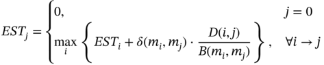
where task 0 denotes the root task of the DAG, which is a virtual task. Its processing time is set 0 and it's the parent node of the entry nodes. δ(m_i, m_j) is an indicative function where δ(m_i, m_j) = 1 denotes m_i ≠ m_j and δ(m_i, m_j) = 0 denotes m_i = m_j. Because the IoT applications begin sensing data by the IoT devices, the entry tasks in DAG are processed in the things tier. It's assumed that the entry tasks of a certain application are allocated in the same cluster.

14.5 Details of Proposed Algorithm

The proposed algorithm that aims to maximize the sum of utility is introduced in this section. First, the encoding and decoding procedure is introduced. After that the uEDA including initialization and repair procedure is presented. Finally, a local search aiming at decreasing total tardiness and increasing successful rate is introduced.

14.5.2 uEDA Scheme

To achieve optimal processing permutation, EDA is adopted to produce a range of individuals and learns from the elite individuals. We use a probability model to describe the relationship between the task pairs. Based on this model, the problem information is used to initialize the probability, and the new population is sampled. Population-based incremental learning (PBIL) is used to update the probability values. The details of the proposed algorithm is given as follows.

14.5.2.1 Probability Model and Initialization

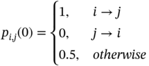
A task permutation probability model P, considering the task relative position relationship, is built to describe and determine the task processing order. Each probability is defined as (14.6), where p_i,j(g) represents the probability that task i is ahead of task j in the permutation at the gth generation of the evolution. It's known that the probability matrix is symmetrical and the diagonal of the matrix is set as 1 for the convenience of calculation.

(14.6)

For the initialization, if there is a precedence constraint between a pair of tasks, the probability value (p_i,j) is initialized as (14.7). In this way, the precedence constraint is settled down during the evaluation.

(14.7)

14.5.2.2 Updating and Sampling Method

To evaluate the population and produce new individuals, the probability model learns from the elite population and is updated. The elite population consists of the N × η% best individuals, where η% is the elite population proportion. The updating scheme is presented as (14.8) and (14.9) where a certain task pair (i, j) is recorded as as (14.9). The sum of indicators is divided by the amount of elite individuals to achieve the frequency of a certain task pair and it's used to update the former probability as the PBIL method [18]:

(14.8)

(14.9)

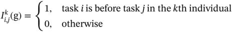
where α ∈ (0, 1) represents learning rate and is the indicator function corresponding to the k-th individual of the population. To achieve new individuals, a sampling method is designed based on the relative position probability model. And the detailed procedure could be referred in [11].

14.6 Simulation

14.6.2 Simulation Environment and Experiment Settings

The testing environment setting and its variables are set as Table 14.1. For each instance, the application is produced by the IoT devices in one cluster and it is processed on the certain one IoT device cluster. Based on the environment settings, the transmission rate between the IoT devices in the same cluster is 1/1 = 1. Because different clusters of IoT devices are located far away from each other, they send information to each other through its fog nodes and thus the transmission rate between IoT devices in different clusters is 1/1 + 2/1 = 3. In addition, the transmission rate between IoT devices and its fog node is 1/1 = 1 and between IoT devices and other fog nodes is 1/1 + 1/5 = 1.2. And the transmission rate between things and cloud tier, fog nodes, fog and cloud tier and cloud nodes are 1/1 + 1/5 = 1.2, 1/5 = 0.2, 1/5 = 0.2, and 1/10 = 0.1. The data transmission time could be calculated as data size multiplies the transmission rate.

Parameter	Implication
Number of clusters in things tier	6, and different number of IoT devices in each cluster ({3, 3, 3, 4, 4, 4});
Number of fog nodes in fog tier	6;
Number of cloud services in cloud tier	2;
Processing speed of IoT, fog, and cloud nodes;	{1, 5, 10};
Bandwidth within IoT, fog, and cloud tier;	{1, 5, 10};
Bandwidth between IoT and fog tier;	1
Bandwidth between fog and cloud tier;	5
Pseudorandom task graph generator	TGFF [19]
Task number n of a DAG	200 ± 100
CCR	{0.1, 0.5, 1.0, 5.0}
Data size	Normal distribution with CCR
Maximum number of successors and processors of a certain task	10
High bound of deadline assignment (Hb)	2.0
Low bound of deadline assignment (Lb)	1.0
Hard deadline constrained tasks proportion	10%
Urgency ratio of tasks	{1.0, 1.5, 2.0}
Stopping criterion generations	30
Population size (N)	10
Learning rate (α)	0.05
Proportion of elite population (η%)	20%
Steps of local search (ls)	n/3

The parameters of the utility functions are settled according to DAG information where T_v is settled as (14.10). For the soft deadline constrained tasks, T_e, T_s are settled as (14.11) and (14.12).

(14.10)

(14.11)

(14.12)

where tlvl_i is the t-level value of task i, which is calculated as the largest sum of processing time of the task path from the entry task to task i. In addition, to discuss the performance of the algorithms under different situation, urgency ratio of tasks is set to control the deadlines and calculated as T′_v = T_v/Loose.

For each CCR, 500 independent DAGs and corresponding deadline values are produced and for each DAG instance, 3 Loose values are used. Thus, 500 × 4 × 3 = 6000 instances are used to validate the efficiency of the proposed algorithm.

14.6.3 Compared with the Heuristic Method

The comparison results of modified heuristic method and our proposed algorithm are listed as Table 14.1. The relative percentage deviation (RPD) value and the p-values of two sample paired t-tests under 95% confidence level are listed. The RPD value is calculated as follows where U^uEDA and U^blvl represents the utility sum obtained by uEDA and the modified heuristic method. And the alternative hypothesis is the sum of task utility of heuristic method is less than our solution. If the hypothesis is accepted, the “Sig” appears to be “Y,” otherwise appears “N.”

(14.13)

From Table 14.2, it could be seen that sum of utility of uEDA is larger than the heuristic solutions under 95% confidence level. Our algorithm performs much better when the deadline is tight and CCR is large. Considering the comparison results, it could be seen that our proposed algorithm is an efficient algorithm for this problem compared to the modified heuristic method.

In addition, based on the results, two chats are presented as follows. Figure 14.2 presents the trends of average RPD value overall Loose situation of either “RPD>0” or “RPD<0.” In Figure 14.3, the blue, yellow, and green column each presents the percentage of “RPD < 0,” “RPD=0,” and “RPD > 0” overall Loose situation.

It could be seen from Figure 14.2 that for each CCR situation, the absolute value of average positive RPD is much larger than negative RPD, which denotes that the superiority of uEDA is much larger than the modified heuristic algorithm. In addition, as CCR grows, the superiority increases. And from Figure 14.3, it could be seen that the solutions obtained by uEDA dominate the modified heuristic method in most cases. And when CCR grows, the superiority of uEDA turns to be more obvious.

	1.0			1.5			2.0
RPD	p-Value	Sig	RPD	p-Value	Sig	RPD	p-Value	Sig
0.1	0.694	0.000	Y	3.769	0.000	Y	3.613	0.000	Y
0.5	0.458	0.000	Y	3.446	0.000	Y	3.491	0.000	Y
1.0	3.232	0.000	Y	14.599	0.000	Y	14.113	0.000	Y
5.0	78.139	0.000	Y	62.214	0.000	Y	56.982	0.000	Y

14.7 Conclusion

In this work, a problem specific uEDA is proposed to address the latency optimization of IoT applications under the three tier systems. The task utility is adopted to measure the performance of the task scheduling algorithm. Our proposed uEDA consists of the basic EDA, problem-specific decoding method and local search procedure. Based on the comparison results of the modified heuristic algorithm, it could be proved the efficiency of our proposed algorithm on this problem. In the future, we plan to consider the computing node capacity, as well as the robustness performance of the scheduling algorithm during the optimization. In addition, the prototype system is needed to achieve realistic benchmark instances and to test our algorithm.

References

1. 1 Mattern, F., Floerkemeier, C., Sachs, K. et al. (2010). From the Internet of computers to the Internet of Things. In: From Active Data Management to Event-Based Systems and More, vol. 6462 (eds. K. Sachs, I. Petrov and P. Guerrero), 242–259. Berlin, Heidelberg: Springer.
2. 2 D. Chu, Toward immersive mobile virtual reality, Proceedings of the 3rd Workshop on Hot Topics in Wireless (HotWireless '16), ACM, New York, October 3–7, 2016.
3. 3 Tran, T.X., Pandey, P., and Hajisami, A. (2017). Collaborative multi-bitrate video caching and processing in mobile-edge computing networks. In: Annual Conference on Wireless On-demand Network Systems and Services (WONS), 165–172. IEEE Congress on Jackson.
4. 4 M. Gorlatova and M. Chiang, Characterizing task completion latencies in fog computing, ArXiv.org: 1811.02638, (2018).
5. 5 Bonomi, F., Milito, R., Zhu, J., and Addepalli, S. (2012). Fog computing and its role in the internet of things. In: Proceedings First Edition of the MCC Workshop on Mobile Cloud Computing, 13–16. Helsinki, Finland, August 17,: ACM.
6. 6 Kwok, Y.K. and Ahmad, I. (1999). Static scheduling algorithms for allocating directed task graphs to multiprocessors. ACM Computing Surveys 31: 406–471.
7. 7 Yang, J., Xu, H., and Jia, P. (2013). Efficient search for genetic-based machine learning system via estimation of distribution algorithms and embedded feature reduction techniques. Neurocomputing 113: 105–121.
8. 8 Armananzas, R., Inza, I., and Santana, R. (2008). A review of estimation of distribution algorithms in bioinformatics. Biodata Mining 1 (1): 6–12.
9. 9 Wang, S.Y. and Wang, L. (2016). An estimation of distribution algorithm-based memetic algorithm for the distributed assembly permutation flow-shop scheduling problem. IEEE Transactions on Systems, Man, and Cybernetics: Systems 46: 139–149.
10. 10 Wu, C.G. and Wang, L. (2018). A multi-model estimation of distribution algorithm for energy efficient scheduling under cloud computing system. Journal of Parallel and Distributed Computing 117: 63–72.
11. 11 Wu, C.G., Li, L., Wang, L., and Zomaya, A. (2018). Hybrid evolutionary scheduling for energy-efficient fog-enhanced internet of things. IEEE Transactions on Cloud Computing 43 (8): 1575–81.
12. 12 Wu, C.G. and Wang, L. (2019). A deadline-aware estimation of distribution algorithm for resource scheduling in fog computing systems. In: IEEE Congress on Evolutionary Computation (CEC), 1–8. IEEE.
13. 13 Yousefpour, A., Fung, C., Nguyen, T. et al. (2019). All one needs to know about fog computing and related edge computing paradigms: a complete survey. Journal of Systems Architecture 98: 289–330.
14. 14 Ye, D., Wu, M., Tang, S., and Yu, R. (2016). Scalable fog computing with service offloading in bus networks. In: Cyber Security and Cloud Computing (CSCloud), IEEE Conference on Beijing, 247–251.
15. 15 Pinedo, M. and Hadavi, K. (1992). Scheduling: theory, algorithms and systems development. In: Operations Research Proceedings 1991 (eds. W. Gaul, A. Bachem, W. Habenicht, et al.). Berlin, Heidelberg: Springer.
16. 16 Koulamas, C. (1994). The total tardiness problem: review and extensions. Operations Research 42: 1025–1041.
17. 17 Sen, T., Sulek, J.M., and Dileepan, P. (2003). Static scheduling research to minimize weighted and unweighted tardiness: a state-of-the-art survey. International Journal of Production Economics 83: 1–12.
18. 18 Liu, J. (2000). Real-Time Systems. Prentice Hall.
19. 19 Li, W., Santos, I., Delicato, F.C. et al. (2017). System modelling and performance evaluation of a three-tier Cloud of Things. Future Generation Computer Systems 70: 104–125.