
CHAPTER TWELVE
Portfolio Resource Allocation
Good portfolio decisions begin with a conducive culture, effective behaviors, a decision quality framework, and a good process
—Michael Menke
12.1 Introduction to Portfolio Decision Analysis
In earlier chapters, we show how to use decision analysis to select the best single choice from a set of well-defined alternatives. But in many cases, the goal is not to select the single best alternative, but rather, to select the combination, or portfolio of alternatives that best meets the articulated goals of the leadership. Many names are used for the alternatives being considered: programs, projects, assets, and opportunities. This is a more complicated problem in which issues such as dependencies (e.g., Project A’s performance depends on Project B funding), ordering (e.g., Project C must be done before Project D), and resource constraints (e.g., budget and/or manpower) must be considered. If there are dozens, or even hundreds of projects, many of which are interdependent, Chapter 6–11 give good guidance on evaluating each individual project, but the complexity of modeling their interactions may be overwhelming. In this chapter, we summarize several approaches that have been used successfully in government, oil and gas, and pharmaceutical industries among others to make the portfolio problem manageable. See Salo et al. (2011) for discussion of Portfolio Decision Analysis and examples.
This chapter is organized as follows. Section 12.2 describes the socio-technical challenges with portfolio decision analysis. Section 12.3 presents portfolio decision analysis with a single financial objective and capital constraints and illustrates the greedy algorithm approach using the Roughneck North American Strategy (RNAS). Section 12.3 presents a multiple objective decision analysis with resource constraint approach using an incremental benefit/cost portfolio analysis and illustrates the approach with the data center portfolio example.
12.2 Socio-Technical Challenges with Portfolio Decision Analysis
One of our major themes of this book is that decision analysis is a social-technical process. If decision analysts approach portfolio decision analysis as a technical problem, they seldom get to implement their approach. As we describe in this chapter, portfolio decision analysis significantly increases both the technical and the social challenges. In this chapter, we focus on the technical challenges, but the success of portfolio decision analysis depends much more on overcoming the social challenges of decision making in large organizations (see Chapter 4). In addition, the increased social complexity typically requires the soft skills of an experienced decision analyst.
In Chapter 9 and Chapter 11, we consider five dimensions of decision complexity: business units, objectives, alternatives, time, and uncertainty. All five of these dimensions apply to portfolio decision analysis. However, many of the dimensions can be more complex for portfolio resource allocation.
- Business units. Portfolio decision analysis can be performed within a business unit or across several business units. These could be business units within a corporation; oil fields in a geographic region; compounds in a drug company’s pipeline; or military or government programs vying for organizational funding. We must evaluate both the individual projects and the aggregate portfolio for each business unit.
- Objectives. Instead of the business unit objectives for one alternative decision, we must consider the business unit objectives for the portfolio of projects (e.g., avoiding loss of key skills if a portfolio is too unbalanced across staffing in an organization). This may significantly expand the scope and number of objectives and involve more decision makers, stakeholders, and subject matter experts.
- Alternatives. As noted above, the number of alternatives can be very large and the number of possible portfolios can be extremely large. For example, suppose we have 10 projects and four funding levels for each project (none, 90%, 100%, and 110%), then the number of possible portfolios is 410. Of course, not all of the portfolios may be interesting (e.g., 0% funding for all) or satisfy the constraints.
- Uncertainty. As we consider large numbers of projects, more business units, and a broader set of objectives, the number of project and business uncertainties can become very large. Assessing all of the required joint probability distributions may become unwieldy.
- Time. The time period for the portfolio decision analysis usually varies from 1 year to many years. Private companies typically use a shorter planning horizon than public organizations. For example, resource allocation planning for government programs is done for at least 5 years into the future (and sometimes for 25 years, for example, for defense program planning). However, project execution portfolio decision analysis might consider only 1 year.
In practice, in addition to the increase in complexity, there are additional social challenges to portfolio analysis:
- Identifying all of the projects can be challenging for organizations that do not have an existing systematic resource allocation process.
- Collecting consistent, credible information on the projects can involve many people who may not have incentives to provide timely information and can take a long time.
- Identifying the project dependencies and portfolio constraints is also difficult. Decision analysts should try to minimize the constraints, since adding a constraint can reduce the total value.
12.3 Single Objective Portfolio Analysis with Resource Constraints
Although we may find it compelling, the perfect capital markets point of view is rarely taken by clients. Instead, clients often view themselves as facing capital constraints.
12.3.1 CHARACTERISTICS OF PORTFOLIO OPTIMIZATION
If we have framed the decision, defined the portfolio alternatives, and obtained all the data, we can identify the capital-constrained global optimum portfolio by considering all possible portfolios, discarding those that are inconsistent with the capital constraint, and choosing the feasible portfolio with the best ENPV. If carefully done and properly explained, this global optimization approach can be useful. However, in practice, there are challenges to it:
- For large problems, it can take considerable computation (and sometimes special algorithms) to find feasible and, especially, optimal solutions.
- Clients sometimes state constraints that are not necessary. This destroys value. For instance, if an oil and gas manager arbitrarily requires that the aggregate success rate of an exploration portfolio exceed a certain threshold, this might rule out profitable high-risk high-reward exploration strategies.
- Small changes to inputs can require time-consuming reoptimization of the entire portfolio.
- The rationale of the recommended portfolio choices may not be clear, especially if a number of unnecessary constraints have been specified.
- Response to changing conditions is sometimes counterintuitive (e.g., if we increase the funding, a funded project may be removed from the portfolio and an unfunded project may be added). This can make for a very unstable solution.
12.3.2 GREEDY ALGORITHM USING PROFITABILITY INDEX AND THE EFFICIENT FRONTIER
Many of the challenges associated with global optimization can be met by developing a figure of merit for projects, rank-ordering them, and choosing from the top down until available funds are exhausted. In computer science, this approach is known as the “greedy” algorithm. Greedy algorithms are quick to calculate, their response to changing assumptions is easy to understand, and they often give results very close to the optimum. Furthermore, we do not have to re-evaluate the entire portfolio to ascertain the status of a new project; we merely compare its figure of merit with the prevailing threshold.
We can develop such a figure of merit by taking a brief look at the mathematics of constrained optimization. This discussion applies equally well to monetary or nonmonetary constraints (e.g., in oil and gas production, headcount or access to drilling equipment may be the constraint). If there are multiple constrained resources, this approach becomes noticeably more complicated. It can still be used as the basis of a computer algorithm, but it loses much of its attractiveness as a way of discussing a portfolio problem with stakeholders.
The derivation of the approach requires a brief reference to the mathematics of optimization. The pragmatic portfolio analyst with less mathematical background can skip the boxed discussion.
(12.1) ![]()
(12.2) ![]()
The limited resource constrains the value we can achieve. At the optimal solution, the shadow price is the value return we would get for one more dollar of budget constraint. A project’s productivity index (PI)1 is the ratio of the value returned per unit resource. We can use the PI to prioritize projects for funding, by choosing those with the best PI until the resource is exhausted, in greedy fashion (Reinsvold et al., 2008). This is equivalent to the PI equal to the shadow price.
The PI approach has often been used in cases where the constraint is financial, by splitting out a component of the cash flow that comprises investment, and treating its present value as the constrained resource. When formulated this way, the shadow price of capital specifies the minimal acceptable level of PI. While there is rarely an actual constraint on present-value investment per se, this formulation can still develop a figure of merit that is helpful. This approach was used in a prominent SmithKline Beecham portfolio review (Sharpe & Keelin, 1998), which is discussed in Chapter 1.
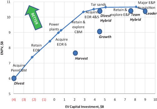
If we plot the total PV of investment dollars on the x-axis and the total ENPV of the portfolio on the y-axis, it is often informative to map out and display an “efficient frontier,” which is the set of portfolios that provide more ENPV value than any other portfolio with equal or lower PV investment. Figure 12.1 gives an example. While this notion of efficiency may differ slightly from what is mathematically optimal,2 the display can nonetheless be insightful.3 The efficient frontier can always be identified by complete enumeration: by evaluating all possible portfolios, putting them all on a scatter plot, and noting those on the upper left extremes. If interproject dependencies are not too complicated, it can also be generated directly by rank ordering the opportunities using PI as we did above, and mapping out the curve that results from adding them one at a time to the portfolio, from best to worst. This chart is useful if the exact level of available investment capital is not yet known—once it becomes known, we look up the portfolio that uses it up and fund the opportunities comprising it. This chart is sometimes called the bang-for-buck curve, investment efficiency curve, or the Chief Financial Officer’s (CFO) curve.
FIGURE 12.1 RNAS investment efficiency curve.
If some opportunities are prerequisites for the feasibility of others, or if the value of one project depends on whether another is chosen, the only completely general way to generate the efficient frontier is by complete enumeration. However, if there are only feasibility dependencies, and not too many of these, we may be able to construct an efficient frontier directly by manually combining prerequisite projects with their more-attractive follow-on projects and then treating these as single projects in constructing the bang for the buck curve.
This entire discussion addresses ENPV value for a given discount rate. Do we have a role in the specification of the discount rate? In the pure decision analyst role, we elicit alternatives, information, and preferences (including discount rate, which expresses time preference for money) from clients and develop and communicate insights from them. A decision analyst per se does not question preferences.
This can be contrasted with a broader role—the decision professional—in which we might also offer guidance on the formulation and articulation of preferences. Some preferences are easy to specify, and should not be questioned. Others, such as discount rate, are difficult to specify, due to their abstractness, and differing schools of thought on the nature and role of discount rate (e.g., the “risk adjusted” discount rates one sees in the finance literature). The following sidebar discusses choice of discount rate in the context of other preferences that are easier to specify, such as preferring more money to less.
12.3.3 APPLICATION TO ROUGHNECK NORTH AMERICAN STRATEGY PORTFOLIO
See Table 1.3 for further information on the illustrative examples. If we interpret the RNAS strategy table (see Chapter 8) as specifying different levels of investment at each of their business units (BUs), but discard the suggestion that high investment in one should be coupled with high investment in another, we can view the RNAS situation as a portfolio problem. There was no binding constraint other than capital, so we calculated the PIs of major RNAS investments (see Table 12.1). This was done by creating a set of strategies that included one opportunity from each business unit, then two, then three, and so on, and simulating the resulting set of strategies. Then looking at the delta between adjacent pairs of strategies and confining the display to the appropriate business unit (BU) gave the incremental cash flow, ENPV, and PV investment for each project, and allowed its PI to be calculated.
TABLE 12.1 RNAS Portfolio Metrics ($M)

In this table, we see that merely retaining E&P assets and producing them was not worthwhile in itself, but it enabled profitable exploration and down-spacing,4 so we merged these into one item “Retain & explore E&P” in the investment efficiency curve. Figure 12.1 shows the resulting RNAS investment efficiency curve, along with the strategies that were analyzed.
Often, the most effective use of a graphic like this is to identify projects that are clear winners and clear losers, and engender team consensus for funding and not funding, respectively. For RNAS, EOR and CBM were clear winners, while the Major E&P Acquisition was a clear loser. The projects in between have roughly zero value. The value of a portfolio is roughly the same if one of these projects is added or if it is removed. This means that little is lost by making such choices suboptimally. In a situation where the client has only a finite amount of time and patience to sort through fine points of valuation, it can be more helpful simply to identify winners, losers, and marginal projects, and allow the organization’s momentum to carry the day on the latter, than to try to force decisions to honor every small difference in value metrics.
12.3.4 PORTFOLIO RISK MANAGEMENT
It may be possible to reduce portfolio risk by selecting opportunities whose values are influenced in opposite ways by uncertainty. A common example of this at the corporate level is vertical integration. For instance, when the price of oil rises, the value of an oil production company rises, while the value of a refinery falls. If an oil producer and refinery merge, the aggregate impact of oil price is largely neutralized, because the two business units naturally hedge one another. There can be opportunities like this within a portfolio, but none was seen at Roughneck.
If an uncertainty influences all opportunities’ value in the same direction, there are no synergies at the portfolio level. Of course, the sensitivities may suggest improvements at the level of individual opportunities.
12.3.5 TRADING OFF FINANCIAL GOALS WITH OTHER STRATEGIC GOALS
Some strategic goals are difficult to measure alongside financial goals. In principle, we could map out the possible outcomes and assess a utility function for all outcomes, and then we would be in position to optimize. In financial portfolio analyses, we often size up strategic goals qualitatively at the end, and adjust decisions to ensure greater alignment with those strategic goals.
For instance, the investment efficiency curve in Figure 12.1 suggests that Divest Hybrid might be the most attractive of the strategies considered. However, upon seeing this, Roughneck management reiterated that oil and gas production (measured in barrel-of-oil equivalents, or boe) was a fundamental objective (see Fig. 12.2), and divesting E&P created too large a drop in production to be accepted.
FIGURE 12.2 RNAS E&P production.

12.4 Multiobjective Portfolio Analysis with Resource Constraints
In the previous section, we describe an approach for achieving portfolio value that focuses on the use of ENPV and Profitability Index (PI) as a basis for selecting competing projects in a portfolio. In this section, we introduce and apply to the data center problem an additional approach that some of the authors have used in many highly successful portfolio analyses. The approach focuses on incremental benefit/cost analysis using Pareto optimality criteria (Buede & Bresnick, 2007; Phillips, 2007). This is entirely analogous to the PI approach, insofar as it treats cost as a constrained resource and develops a figure of merit by dividing benefit by cost. An alternative multiobjective decision analysis approach is to use a multiobjective value model to assess the value of the projects and an optimization model that determines the best value for the resource constraints (Burk & Parnell, 2011).
12.4.1 CHARACTERISTICS OF INCREMENTAL BENEFIT/COST PORTFOLIO ANALYSIS
The cost–benefit analysis approach to portfolio resource allocation focuses on determining the incremental benefit/cost ratios of competing program elements and on establishing the most cost-efficient way of spending additional resources, referred to as an “efficient order-of-buy.” It can be used as a zero-based analysis tool, or can be used to examine allocations beyond some defined baseline. It can also be used in a budget-cutting mode to develop an “efficient order of sell.” The solution approach explicitly identifies the set of feasible alternatives that are built to reflect the constraints, evaluates only the alternatives that provide the most “bang-for-the-buck” at any level of resource expenditure, and provides a clear audit trail for the results. This technique is best suited for problems:
- that have a very large number of alternative allocation schemes;
- where funding areas are independent (i.e., funding one area does not impact the benefit of funding another area);
- where programs can be divided into increments such that a piece of a program can be funded without funding the entire program;
- where budget constraints are expected to change greatly or are not known initially;
- where reasons for the resulting allocations need to be completely transparent; and
- where it is useful for participants to understand the underlying mathematical algorithms.
12.4.2 ALGORITHM FOR INCREMENTAL BENEFIT/COST PORTFOLIO ANALYSIS
12.4.2.1 Identify the Objective.
For illustration purposes, assume that we are trying to maximize some notion of portfolio “benefit” subject to cost constraints (e.g., dollars, time, and people) and physical constraints (e.g., space, power, weight, and bandwidth). For convenience, we will call the areas to which we are allocating resources “programs,” each of which can be funded at various “levels” of expenditure. Each program level that gets funded will contribute some “benefit” toward satisfying organizational needs. Our objective is to get the most “bang-for-the-buck” for any level of expenditure.
12.4.2.2 Generate Options.
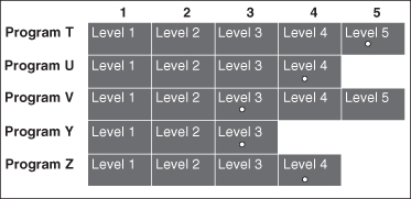
We assume that there are a limited, but perhaps large number of programs, i, to which we can allocate resources. We also assume that the programs are value independent, which implies that the level at which program A is funded should not affect the benefit associated with levels of program B.5 For each program, there are at least two levels at which we can fund, which may range from none (do not fund) to “gold-plated” (with all the bells and whistles). A program is represented by a “row” in the matrix below, with the various funding alternatives being shown from left to right as levels for the row. A row may simply have two levels (for a Go/No-Go program that cannot be divided), or many levels for one with well-defined funding increments. Practically, the number of levels per row should be less than 10, although there is no analytical requirement for this. The levels may be independent of each other (called substitute levels, where we do level 1 or level 2 but not both), or inclusive (called cumulative levels where funding level 2 includes level 1). A set of alternative programs and funding levels is shown in Figure 12.3 in matrix form.
FIGURE 12.3 Funding areas and levels.

A specific portfolio is then defined by selecting one level in each row. One such portfolio is represented by the white dots in Figure 12.4. Each portfolio has an associated cost which is the sum of the costs of each selected program and level.
FIGURE 12.4 One possible portfolio.
As shown in the introduction, the number of possible funding options is the product of the number of funding levels of the programs.
Each such combination can be thought of as a funding option or package. Clearly, we do not want to evaluate every possible combination since this can easily reach the thousands or millions. The approach described here makes it unnecessary to do this; instead, it identifies and considers only those options that are determined to be “efficient.”
Let us assume that we can calculate the “benefit” of each level using the techniques described earlier in the handbook, either through NPV, expected value, or MODA techniques. We can then plot the cost and benefit of any package, such as our “white dot” alternative on a benefit–cost graph as shown in Figure 12.5.
FIGURE 12.5 Benefit vs. cost plot of one possible portfolio.

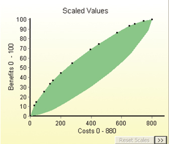
If we plot all possible portfolios (i.e., combinations of one level selected from each row), they have the “nice” mathematical property of falling within the football shaped region shown in Figure 12.6.
FIGURE 12.6 Trade space of portfolios.
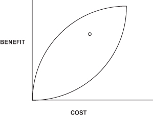
It is easy to see that for any cost C, we want to find the package that is as high on the benefit scale as possible; that is, we want to find the package X that falls on top of the football, known as the efficient frontier or the Pareto optimal frontier, as shown in Figure 12.7. Note that package X has the same cost as the white dot package, but gets more benefit. Also note that there is a package Y that gets the same benefit as the white dot package, but is cheaper. In fact, any package in the triangular wedge formed by X, Y, and the white dot is more “efficient” than the “white dot” solution.
FIGURE 12.7 Selected portfolio for Cost C, better portfolio for same Cost (X), cheaper portfolio with same benefit (Y).

The programs under consideration may come from a variety of internal and external sources. Programs may be couched in terms of the current baseline, additions to the baseline, deletions from the baseline, or other modifications to the baseline. It is usually wise to include the baseline (or “do nothing”) option in the analysis to provide a benchmark for comparison with the other options.
12.4.2.3 Assess Costs.
Assessing the costs associated with each program element is conceptually easy, yet may be very difficult to do in practice. At a minimum, the following issues should be addressed:
- Will life cycle cost estimates be used, and if not, which costs should be included?
- Can different “colors6” of money be combined or do we need to consider them separately?
- What assumptions will be made about inflation to enable comparison of constant dollars with current-year dollars?
- What assumptions will be made about discount factors to accommodate time-value-of-money considerations?
- Who provided the cost estimates, and was an independent cost estimate made as well?
- If costs were provided by different organizations, were the same “ground rules” followed?
The benefit/cost methodology allows for multiple dimensions of the constrained resource (such as various budget year dollars or different “colors” of money2), or even different types of resources (people vs. dollars vs. time). However, in order to combine costs, they all must have the same dimensionality. With dollars, this is no problem. With different types of resources, there are three choices. First, we can convert all resources to dollars. Second, we can allocate based on one resource at a time, and see where differences in the allocation schemes occur as we vary the resource considered. Third, we can establish a relative “value” scale on costs that allows us to treat one type of resource as more or less important than another by assigning weights to the different types of resources. Regardless of the method used, when calculating the benefit–cost ratios of the packages, a single resource number should be used.
12.4.2.4 Assess Benefits.
This is typically the most difficult and most controversial part of the process. Often, there are insufficient “hard data” available to provide purely objective measures of benefit for the programs. Thus, it is necessary to rely upon more subjective and judgmental assessments from experts. Both the measures of performance used to evaluate the programs and the elicitation techniques themselves must be selected carefully and executed in a technically sound and defensible manner.
In addition to the techniques for assessing value described earlier in the handbook, there are a variety of techniques that may be used for subjective benefit assessment (Brown et al., 1974; Barclay et al., 1977) and most use some measure of “relative value” to compare programs on one or more dimensions. Whether the measure is called “benefit,” “pain,” or simply “value” is not the important consideration, but rather, whether or not the measures are set up and defined in a way that facilitates assessment from the experts.
For the approach described here, we will use multiple attributes of benefit that relate to dimensions of performance (e.g., NPV, environmental impact, and fit with strategic direction). The benefit of a program at each level of funding can be assessed in terms of each of these needs separately, and then later combined across the dimensions. Benefits are assessed one row at a time, and one attribute of benefit at a time. For example, first consider Program X in terms of how well its elements contribute toward fit with strategic corporate goals. The level that provides the greatest satisfaction on “fit” arbitrarily scores 100; the level that provides the lowest level arbitrarily scores 0 (Note: A benefit score of 0 does not mean there is no benefit associated with the level; it means that this is the starting point against which additional benefit can be measured). There is no requirement that 0 be at the leftmost level or that 100 be at the rightmost level. The intermediate levels are scored with relation to 0 and 100 points. Thus, a level scoring 90 implies that funding to that level provides 90% of the total benefit that could be achieved in going from the lowest level to the highest. We then make similar assessments for the other attributes of benefit. When this is done, we move to the next row (program) and make the same assessments. When we are done with all programs, each row has its levels scored on a 0–100 basis for each attribute. At this point in time, it is not possible to compare one row with another or one attribute of benefit with another since they were all assessed on independent 0-to-100 scales. We therefore need a way of “calibrating” these scores to a common metric. This is done first by assigning “within criteria” weights, wik, which compare one row with another on each attribute, and second, by assigning “across criteria” weights, ak, to the different attributes of benefit. We can then calculate the weighted average for each level of a program across all criteria. Thus, on the common scale, the benefit score Bijk for level j of program i across k evaluation criteria would be calculated as:
(12.3) ![]()
where wik is the “normalized” weight assigned to program i for criterion k, and ak is the “normalized” weight assigned to criterion k.7
12.4.2.5 Specify Constraints.
The above formulation does not explicitly include constraints that limit the resource allocation solutions, but instead builds them implicitly into the structure of the problem. For example, if for a given row, doing X or Y requires doing the other, we put them in the same level so both get funded together if at all. In the example below, X and Y never get selected without the other:
| Level 1 | W |
| Level 2 | X,Y |
| Level 3 | W,X,Y |
| Level 4 | Z |
| Level 5 | Z,X,Y |
If we could do X or Y but not both, we build them into separate levels of the row where the levels are substitutes for each other. In the example below, X and Y never get selected together:
| Level 1 | W |
| Level 2 | X |
| Level 3 | Y |
| Level 4 | W,X |
| Level 5 | W,Y |
If doing X requires Y, but Y does not require X, we put them in separate levels where the levels are cumulative, with Y in a lower level than X. In the example below, Y can be selected without X, but X cannot be selected without Y:
| Level 1 | W |
| Level 2 | Y |
| Level 3 | W,Y |
| Level 4 | X,Y |
| Level 5 | W,X,Y |
Clearly, it is essential that the benefits and costs associated with each level reflect these relationships.
This formulation also allows the use of a single constraint in another way. The model can be queried to find the best solution for a specified resource amount (e.g., find the best portfolio for $250M), or to find the cheapest way to achieve a specified level of benefit (e.g., find the cheapest portfolio which will get us 90% of the potential benefit). In both cases, the specified amount acts as a constraint on the preferred portfolio.
12.4.2.6 Allocate Resources.
The algorithm used is relatively straightforward. First, both the “across criteria” weights and the “within criteria” weights are applied to the assessed benefits for each level of each row. Second, the change in benefit (Δbenefit) and the change in cost (Δcost) are calculated for each increment of each row, where by increment, we mean going from one level in a row to the next. Third, we calculate the ratio of Δbenefit to Δcost for each increment. Finally, we order all of the increments in decreasing Δbenefit/Δcost order. This becomes the “order-of-buy,” or the order in which the levels are funded in a purchasing exercise; the ordering can also be reversed to produce an “order-of-sell” for a budget-cutting exercise. Once a resource constraint such as a budget line is applied to the ordered listing, the resource allocation task becomes one of funding everything above the line, and not funding everything below the line. This results in a very stable program since changes in the budget do not require a total realignment of funding decisions; rather, changes simply result in moving the budget line up or down and determining which increments enter or leave the suggested mix at the margin.
An important complication can arise in this process. The algorithm assumes that we always want to fund in decreasing Δbenefit/Δcost order, and assumes that for each row, the levels are built to reflect such an order. If we look at a benefit/cost plot for such a row, this would result in a concave downward curve with an ever-decreasing slope (Fig. 12.8). In reality, this is not always possible to achieve, and in fact, where levels are substitutes for each other, is not likely to happen, and there will be “dips” in the curve (Fig. 12.9). The algorithm assumes that we do not want to fund less efficient increments before we fund more efficient increments, so it adjusts the curve to smooth out the dips. It does this by combining any levels where the subsequent slopes are increasing and then calculating the Δbenefit/Δ cost for the “combined” increment (Fig. 12.10). The combined increment is then placed in the order-of-buy in the appropriate place, and if it is funded at all, it will be funded completely. In a row with cumulative levels, this means that we never stop at the intervening level, but do it all. In a row with substitute levels, we completely skip over the less efficient level and fund the more efficient level. In the most commonly used COTS software packages for this approach, this happens automatically since the costs are built into the levels to reflect the nature of the row.
FIGURE 12.8 Curve with decreasing slope.
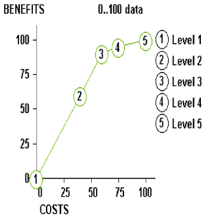
FIGURE 12.9 Curve with varying slope.

FIGURE 12.10 Combination of levels for curve with varying slope.

12.4.2.7 Perform Sensitivity Analysis.
A critical part of the analysis is to challenge the initial assumptions by performing a sensitivity analysis. This can take various forms. By generating the order-of-buy, we can create a contingency table that reflects the best package arrayed against various budget targets. We can also do sensitivity analysis on the benefit measures either by varying the benefits associated with the programs, or by varying the “within criteria” or “across criteria” weights. We can also vary the assumptions on costs to include discount rates or costing models and see how the solution changes.
12.4.3 APPLICATION TO THE DATA CENTER PORTFOLIO
See Table 1.3 for further information on the illustrative examples. Assume that we have selected a single data center location and now must determine the portfolio of projects for the data center that we can fund. As is typical, the projects submitted for funding greatly exceed the resources available. There are four major business areas in the data center—Applications, Security, Platforms, and Connectivity, and they are all competing for the same funds. Three criteria have been identified to evaluate the programs: (1) maintenance of legacy systems (maintain); (2) advance strategic direction of the data center (strategic fit); and (3) ease of implementation, including integration issues. Life cycle NPV has been calculated for each proposed program as the cost dimension of the analysis. Table 12.2 summarizes the input data for the portfolio analysis. For the benefits, the pros and cons of each alternative were discussed in terms of each of the criteria, and the scales in Table 12.3 were developed:
TABLE 12.2 Projects Requesting Funding

TABLE 12.3 MODA Value Scales

Table 12.4 shows how each project was valued on the scales:
TABLE 12.4 Values for Projects

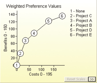
Using the swing weighting techniques described in earlier chapters and the weighting procedure described in Section 12.3.2, assume we assess weights of 10 for Maintain Legacy, 60 for Strategic Fit, and 30 for Ease of Implementation. For ease in analyzing results, the benefits in the model are normalized to sum to 1000 across all criteria. The trade space of projects is shown in Figure 12.11.
FIGURE 12.11 Trade space of data center projects.

Note that an option is included to fund no projects in an area. Within each business area, the projects are ordered by decreasing incremental Benefit/Cost ratios. For example, in Applications, the incremental benefit divided by the incremental cost of going from project C to Project A is greater than that of going from Project A to Project B. In the example, we assume that all projects are value-independent, but this is not a requirement for the approach. The example is also built in a cumulative fashion in that funding Project A implies that Project C has been funded as well (again, not a requirement of the approach—projects can be cumulative or exclusive of each other).
We can examine the data for the model by looking at Figures 12.12 and 12.13, which show the structure of the Applications business area.
FIGURE 12.12 Data for applications projects.
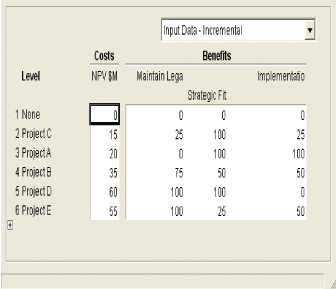
FIGURE 12.13 B/C for applications projects.
As described in Section 12.4.2, when we put all of the data for all business areas together, we produce the full trade space of portfolios along with the efficient frontier as shown in Figure 12.14. Each “dot” on the top of the football-shaped area (the “efficient frontier”) represents adding the next best project based on incremental B/C ratio to the portfolio. For example, for a budget of $450M, we would fund all projects represented by the black dots going from the origin to the $450M point on the frontier.
FIGURE 12.14 Efficient frontier for the data center.
We next explore the efficient frontier by looking at the order in which projects would be funded, or the “order of buy” as in Table 12.5.
TABLE 12.5 Project Order-of-Buy

Assuming that the budget is $450M, the funded portfolio across business areas would be as shown in Table 12.6.
TABLE 12.6 Best Portfolio for $450M
| Area | Funded Projects | Cost $M |
| Applications | C, A | 35 |
| Platforms | F,H | 90 |
| Security | M,N | 170 |
| Connectivity | R,T,S | 155 |
As with all approaches, the next step would be sensitivity analysis on the weights, scores, criteria, and so on. Additionally, we would make some after-the-fact dependency checks, and revise the portfolio accordingly. If the portfolio that emerges from analysis of a multiobjective decision analysis seems to give disproportionate weight to one value measure, this may serve as an opportunity to revisit the weights of the value measures in the value model.
12.4.4 COMPARISON WITH PORTFOLIO OPTIMIZATION
This approach, which is basically a “greedy hill climbing” algorithm, is very similar to the multiple objective decision analysis and optimization resource allocation approach used in Chapter 8 of Kirkwood (1997). In optimization, all constraints are added by equations instead of structuring the alternatives in rows. A binary linear programming algorithm is then used to find the optimal portfolio for any budget level. The optimization approach has the strength that constraints can also be used to model the dependence of funding areas. However, the optimization approach does not always provide a stable allocation; as the budget increases, a program can enter the portfolio, leave the portfolio, and then reenter the portfolio. While mathematically correct, this property is hard to explain to program advocates when more money becomes available and their program drops from the selected set of programs.
12.4.5 STRENGTHS AND WEAKNESSES OF INCREMENTAL BENEFIT/COST PORTFOLIO ANALYSIS
The approach described above has the following strengths:
- Alternatives can be developed either as Go/No-Go or as individual funding increments of a program.
- It provides a very stable allocation scheme; as the budget changes, funding increments enter or leave the mix, but the order of funding stays the same.
- The rationale for the “answer” is readily apparent in that the mathematics of the approach are straightforward and easy to understand.
- It provides an approach for quantifying costs and benefits (both objective and subjective).
- It is available in commercial off-the-shelf (COTS) software.
- It accommodates multiple constraints and dependencies among levels of a funding area.
- It facilitates sensitivity analysis by supporting “what-if” analysis capability.
- It brings some structure and discipline to a difficult process, and provides an audit trail for the results of the analyses.
The approach has the following limitations:
- Since the funding increments are discrete, there may not be a package that falls exactly at the specified budget constraint; the analyst must decide offline whether to (1) “fill the gap” with a level further down in the funding order that stays within budget; (2) modify levels to get closer to the budget target; or (3) modify the budget target.
- It relies heavily on expert judgment.
- It can accommodate only a limited number of attributes of benefit, probably less than 10 before the assessments become overwhelming and the capabilities of available COTS packages are exceeded. This is not due to mathematical constraints, but rather, due to the best practices in human factors that dictate how much should be displayed on a screen, how much scrolling is okay before it becomes distracting, and so on. Most of the COTS packages that implement this approach were designed to be used in group assessment sessions, so human factor concerns were built into the packages.
- The algorithm requires independence of funding areas (but there are various ways available to deal with dependencies if needed).
12.5 Summary
In many cases, the goal of a decision analysis is not to select the single best alternative, but rather, to select the combination, or portfolio of alternatives (e.g., projects), that best meets the articulated goals. In this chapter, we summarize several approaches that have been used successfully in government, petrochemicals, and pharmaceutical industries among others to make the portfolio problem manageable.
In “perfect capital markets,” the weighted average cost of capital (WACC) is the opportunity cost of capital, and it is appropriate to use WACC as a discount rate and fund all projects with a positive expected net present value (ENPV). However, this “rule” becomes more difficult to use when capital is constrained and a firm is unwilling or unable to acquire debt or equity at the WACC in order to fund all acceptable projects.
One way around this problem is to state an acceptable discount rate and identify the constrained global optimum by considering all possible portfolios, discarding those that violate this constraint, and make feasible choices based on best ENPV.
The shadow price approach prioritizes projects for funding by choosing those with the best break-even shadow price until resources are exhausted. We can also use shadow prices by splitting out a component of the cash flow that comprises investment, and treating its present value as the constrained resource. This is known as using a Profitability Index.
Incremental benefit/cost analysis using Pareto optimality criteria has been used in many highly successful portfolio analyses. It establishes the most cost-efficient way of spending additional resources or accommodating budget cuts. The solution approach explicitly identifies the set of feasible alternatives that honors the problem constraints, and evaluates only the alternatives that provide the most “bang-for-the-buck” at any level of resource expenditure.
In this approach, programs that are competing for funding are described in terms of funding levels that could be as simple as Go/No-Go, or more complicated in terms of several funding increments. The increments can be dependent or independent, but the programs are assumed to be preferentially independent. For each funding level, incremental benefit and incremental costs are calculated, and program levels are then funded in order of decreasing Δbenefit/Δcost. This approach is similar to the MODA approach used in chapter 8 of Kirkwood (Kirkwood, 1997), with one major difference. The optimization approach does not always provide a stable allocation; as the budget increases, a program can enter the portfolio, leave the portfolio, and then reenter the portfolio. With the approach described here, the order-of-buy remains constant, but the cut-off line for funding just moves up or down.
KEY TERMS
Notes
1To confirm the equivalence, interpret h as PV investment capital and λ as the PI, set f(x) − λh(x) = 0, and solve for λ. Some firms and references (e.g., http://www.investopedia.com) define the numerator as future cash flow not considering investment, which adds 1 to all PIs. This does not affect interpretation or use.
2A portfolio made up of projects with a good ratio of value to PV investment may not be the same as the portfolio that has the highest value. This can be seen by noting that the former can be influenced by different definitions of which costs are considered to be “investment” while the latter is not.
3The differences from “optimal” are often small. Often it is better to let organizational momentum take its course than to try to force all decisions to honor small differences in value metrics.
4Down-spacing refers to additional drilling in an already developed area. This can increase and accelerate production, thereby increasing its value.
5In reality, there is often a high degree of dependence among some programs, so we must deal with this problem by combining programs together and forming a larger program.
6In government funding, each budget category (research, development, procurement, operations, and so on) has restrictions on the types of programs that can be funded with that category.
7To normalize, sum all of the components and divide each component by the sum.
REFERENCES
Barclay, S., Brown, R., Kelly, C., Peterson, C., Phillips, L., & Selvidge, J. (1977). Handbook for Decision Analysis. Arlington, VA: Defense Advanced Projects Agency.
Brown, R., Kahr, A., & Peterson, C. (1974). Decision Analysis for the Manager. New York: Holt, Rinehart, and Winston.
Buede, D.M. & Bresnick, T.A. (2007). Applications of decision analysis to the military systems acquisition process. In W. Edwards, R. Miles, & D. von Winterfeldt (eds.), Advances in Decision Analysis, pp. 539–563. Cambridge: Cambridge University Press.
Burk, R.C. & Parnell, G.S. (2011). Portfolio decision analysis: Lessons from military applications. In A. Salo, J. Keisler, & A. Morton (eds.), Portfolio Decision Analysis: Improved Methods for Resource Allocation. New York: Springer.
Kirkwood, C. (1997). Strategic Decision Making. Belmont, CA: Duxbury Press.
Luenberger, D. (1984). Linear and Nonlinear Programming. Reading, MA: Addison-Wesley Publishing Company.
Phillips, L. (2007). Decision conferencing. In R. Miles, D. Von Winterfelt, & W.E. Edwards (eds.), Advances in Decision Analysis, pp. 375–398. New York: Cambridge University Press.
Reinsvold, C., Johnson, E., & Menke, M. (2008). Seeing the Forest as Well as the Trees: Creating Value with Portfolio Optimization.
Salo, A., Keisler, J., & Morton, A. (2011). Portfolio Decision Analysis: Improved Methods for Resource Allocation. New York: Springer.
Sharpe, P. & Keelin, T. (1998). How SmithKline Beecham makes better resource-allocation decisions. Harvard Business Review, 76(2), 45–57.