
CHAPTER NINE
Perform Deterministic Analysis and Develop Insights
All models are wrong, but some are useful.
—George E P Box
9.1 Introduction
Our decision analysis approach is to develop and refine a model of how value is created, and to use this to identify even better ways to create value. The model embodies what we call a composite perspective because it incorporates the combined views of many participants. How the model responds to changes in inputs representing decision choices and uncertain factors may not be obvious from the individuals’ points of view. In a word, the behavior of value in the composite perspective is an emergent phenomenon.
We use a “value dialogue” to compare the emergent behavior of the composite perspective to the individual perspectives and, where they differ, improve one or the other to bring them into better alignment. Having done so, we can use the improved composite perspective to understand how much value each alternative creates, and to create even better alternatives. Doing this requires these steps:
- Modeling. Build representations of experts’ perspectives about important events, stitch them together to create a composite perspective on value creation, and represent this in a model.
- Exploration. Explore possible value outcomes in the model in response to different decision choices and uncertainty outcomes.
- Analysis. Characterize the emergent behavior in terms that allow direct comparison with individuals’ perspectives and generation of improved strategies.
Quantitative modeling is an essential step when applying decision analysis to most important organizational decisions, because such decisions are made in the face of considerable complexity and uncertainty. It is well established that the human brain cannot simultaneously process more than a few pieces of information without error. Modeling and analysis allow us to overcome this limitation through a “divide and conquer” approach. A complex problem is decomposed into smaller, simpler pieces that the human brain can comprehend and then put back together in an integrated analytic structure.
Every model is built for a specific purpose. When a new jetliner is being designed, for example, a model is built to test its aerodynamics in a wind tunnel. This model should be quite accurate regarding the aerodynamic surfaces of the aircraft, but need not be accurate regarding its interior structure. The purpose of a decision model is to give insight into the reasons why one possible course of action is better than the others. We seek to develop a requisite decision model. Phillips (Phillips, 1984) defines a requisite decision model as “a model whose form and content are sufficient to solve a particular problem.” It should be accurate enough to differentiate the various alternatives under consideration. It can be quite inaccurate regarding details that do not contribute to a comparison of the alternatives.
A best practice is to follow the dictum, “Be clear about the purpose of the model.” Do not waste time and effort working on features of the model that do not serve its purpose of distinguishing between alternatives. A good strategy for building a decision model is to start simple and to add complexity only where it is needed to improve the insights produced by the model. Also, resist the temptation to use a completed decision model for other purposes. For example, a model that was built for comparing high-level strategies for a business unit would likely be ill-suited for use in optimizing the operations of that business.
A good decision model is one that is both useful and tractable. A useful decision model is one that generates clear insights for decision making. It is both error-free and readily understood by the decision analyst. A tractable model is one that can be built and used within the constraints of time and level of effort for the decision. There is often a trade-off to be made between usefulness and tractability; good engineering judgment is needed to make this trade-off appropriately.
When creating a decision model, always be conscious of two different audiences. The first audience is the computer. The model, of course, must make sense to the computer. It should be free of errors and do what is intended. The second audience is the team of people who look at the model to try to understand how it works. It is certainly possible to create a model that the computer understands and runs flawlessly but which is impenetrable for the analysts and/or decision maker(s). Such a model is not good because if the team cannot understand how it works, they will have little credibility in its results and will be unwilling to make decisions based on them. Also, if it is difficult for the analyst to understand a model, it increases the risk of logical errors being introduced when the model is revised. Therefore, a good decision model is one that can be easily understood by the users.
In decision analysis, we can use models deterministically, probabilistically, or both. We discuss deterministic analysis in this chapter and probabilistic simulation and analysis in Chapter 11.
This chapter is organized as follows. In Section 9.2, we introduce the influence diagram as a tool for planning the model. In Section 9.3, we discuss the advantages of spreadsheet software as a modeling platform. In Section 9.4, we provide our guidelines for building a spreadsheet decision model. In Section 9.5, we describe how we organize a spreadsheet model. For complex models, we need to verify that they are correct, so in Section 9.6, we describe debugging a spreadsheet model. In Section 9.7, we present techniques for deterministic analysis. In Section 9.8, we perform a deterministic analysis of RNAS, our illustrative singe-objective problem. In Section 9.9, we present a simple example to illustrate multiple objective decision analysis having a monetary value metric. In Section 9.10, we present deterministic multiple objective decision analysis with a non-monetary value metric, using the most common model, the additive model. In Section 9.11, we apply the methods presented in Section 9.10 to the data center problem. In Section 9.12, we summarize the chapter.
9.2 Planning the Model: Influence Diagrams
Just as it is an excellent idea to draw up a set of plans before starting the construction of a building, it is wise to make a plan for a decision model before creating it. An especially useful tool for planning a decision model is the influence diagram (Howard & Matheson, 2005), sometimes also called a “value map,” or “decision diagram.” An influence diagram is a graphical representation of the calculation of the value metrics, as they depend on the choice of decision alternative and on external factors, which may be uncertain. Appendix B provides an introduction to influence diagrams. Chapter 10 gives a detailed discussion of how to structure the influence diagram for a decision problem, and how to populate it with pertinent expertise.
An influence diagram is a useful high-level “blue print” for the model. It identifies the key external factors that must be in the model to calculate the value metrics and shows the basic structure of those calculations. It also shows the interdependencies among the uncertain external factors, the decisions, and the values.
However, the influence diagram does not contain all of the information needed to build the model. For example, it does not specify the sequencing or dynamics of the external factors (i.e., how they change over time). Nor does it generally specify the formulas to be used in the calculations.
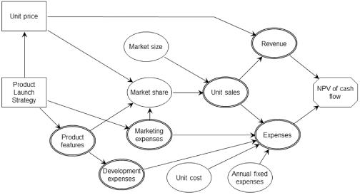
As an example, Figure 9.1 displays the influence diagram for a decision on the launch strategy for a new product (i.e., what features to put in the product and how much to spend on marketing it) and on the selling price of the product. Uncertainty in the product’s market share is affected by its features, by its price, and by the size of the marketing budget. Unit sales are the product of market share and market size, which is also uncertain. Revenue is then calculated as unit sales times unit price. Expenses are equal to the variable manufacturing cost (unit sales times unit cost) plus development expenses, marketing expenses, and other annual fixed expenses.
FIGURE 9.1 Example influence diagram.
9.3 Spreadsheet Software as the Modeling Platform
Spreadsheet software, such as Microsoft® Excel, offers a number of advantages that make it a good choice as the platform for a decision model. The art of modeling in Excel is recognized as a key analyst skill and is taught in many undergraduate and graduate programs (Powell & Baker, 2011).
Spreadsheet software does have some limitations when it comes to decision modeling. Working with arrays having four or more dimensions is difficult. It is difficult to build models with complex dynamic interactions in spreadsheets. And working with very large spreadsheet models tends to be cumbersome and slow. But overall, except for large, complex models, the advantages of spreadsheets compensate for the disadvantages. The remaining discussion assumes that modeling and analysis is done in a spreadsheet environment.
9.4 Guidelines for Building a Spreadsheet Decision Model
We present several guidelines for developing a spreadsheet decision model that are especially useful if many members of the decision team participate in developing and using the model.
9.4.1 KEEP INPUTS SEPARATED FROM CALCULATIONS
All inputs to the model should be located together in one place, clearly separated from the calculations. Think of this as the “control panel” for the model—everything needed to operate the model is there.
A corollary of this guideline is that the calculation formulas in the model should not contain any “hard-wired” numbers. The quantity represented by a hard-wired number in the formula should instead be expressed as an input variable. Even conversion constants should follow this rule. The only numbers that should appear in calculation formulas are 0 and 1. If this guideline is followed, calculation formulas will contain only inputs and the results of other calculations.
Many decision analysts use cell coloring to support this rule. For example, yellow might be the inputs, green the calculations, and blue the decisions.
9.4.2 PARAMETERIZE EVERYTHING
To describe how a quantity (such as the size of a market segment) changes over time, it is tempting to simply type into the spreadsheet a different number for each year. However, this is a bad practice. It is much better to use parameters to describe the dynamics of the quantity. For example, one way to parameterize the dynamics is to create two input variables, one for the initial amount and the other for the annual growth rate. Parameterizing the model dynamics makes it much easier to include the effects of uncertainty in the model.
9.4.3 USE RANGE NAMES FOR READABILITY
Spreadsheet software allows the user to define names to refer to individual worksheet cells or ranges of cells. Using names rather than cell addresses in calculation formulas makes it much easier for a human to understand those formulas, especially when the reference is nonlocal (i.e., from one sheet to another).
For example, the formula for unit sales using named ranges might be:
![]()
This is much easier for a human reader to understand than a formula using cell addresses:
![]()
Every input variable and calculated intermediate result in the model should be given a name. When creating names, use a good naming convention. For example, use distinctive suffixes to designate attributes, such as geographies or product line. Using a well-designed naming convention has several advantages. It enhances the ability of humans to understand the model. It reduces the chance of typographical errors being introduced. And it facilitates creating formulas via copy and paste for additional geographies or product lines.
9.4.4 USE UNIFORM INDEXING FOR ROWS AND COLUMNS OF A SHEET
Uniform indexing means that the row header on the left applies to the entire row, and the column header at the top applies to the entire column. This way, if a row or column is added or deleted, the rest of the sheet retains its validity. Excel’s FreezePanes facility encourages and supports this practice by allowing common row and column indexes at the left and top to be visible regardless of what portion of the sheet is currently displayed. By contrast, putting tables with different indexing structure below or beside the main table makes spreadsheets brittle—the modeler may see a way to improve a structure, but be afraid to implement it for fear of damaging something unrelated below or beside it.
9.4.5 MANAGE THE MODEL CONFIGURATIONS
Configuration management is necessary regardless of how many modelers actually touch the spreadsheet. Configuration management can be as simple as following a naming convention for the spreadsheet file as it is updated and enhanced; for example, decisionmodel_YYYYMMDD_initials.xlsx.
9.5 Organization of a Spreadsheet Decision Model
The model we build must represent up to five dimensions of complexity often found in decision situations:
Three of these dimensions comprise what is called the decision basis: alternatives (decisions and strategies), information (uncertainties), and preferences (values components) (Howard, 1983). We add two more dimensions to the conversation (business units and time) because these are frequently considered explicitly, and the techniques for managing these dimensions can often be useful for facilitating the value dialogue discussed in Chapter 11.
We must think carefully at the beginning about how much granularity to model, and how to represent these dimensions of complexity in the model to ensure that we can deliver insightful analysis, while allowing tractable modeling. More fine-grained information requires more effort to elicit, model, simulate, and analyze, but may allow for expertise to be captured more authentically, and may give more opportunities to improve strategies in the value dialogue.
For some kinds of granularity, it is feasible to begin with less detail, and to elaborate only if initial analysis suggests that the elaboration could be fruitful. However, if we are deciding whether to disaggregate a dimension, this often needs to be decided upon at the beginning of the project.
There are two basic ways to represent any given dimension:
- Intensively. Represent all possible cases but only one at a time.
- Extensively. Simultaneously represent all possible cases explicitly.
While extensive representation of all dimensions simultaneously would make all our desired analyses straightforward, this can become intractable in a spreadsheet, which has only three natural dimensions (sheets, rows, and columns).We usually choose intensive representation for decisions and uncertainties because each of these “dimensions” is actually a multidimensional space. In some cases, a dimension may not be modeled at all. For example, time is not explicitly modeled in the data center case. The important point is to size up what needs to be generated, stored, and understood and to design the spreadsheet accordingly.
The structure and controls of the model must support analysis, and a key aspect of analysis is to summarize, or collapse, a dimension when it is not currently of interest, to allow others to be reviewed conveniently.
This section discusses the pluses and minuses of representing each dimension explicitly, and offers thoughts on how each of the dimensions can be analyzed, and what the implications are for spreadsheet structure and analysis controls.
9.5.1 VALUE COMPONENTS
A decision analysis ultimately produces a utility metric, whose expected value (EV) is optimized for decision making under uncertainty. Sometimes it is generated by aggregating scores for objectives; sometimes by aggregating the present value (PV) of line items in a P&L such as revenue, costs, taxes, and investment; and sometimes by aggregating net present values (NPVs) of business units. Sometimes there is an explicit adjustment reflecting risk attitude, sometimes not. We refer to the items directly used in the calculation of utility as value components.
Considering value components explicitly supports the following lines of thought for adding value in the value dialogue:
- Enhance a favorable item.
- Minimize or mitigate an unfavorable item.
- Optimize for a different value measure.
- Find a better tradeoff between objectives
We almost always want to consider this level of granularity explicitly. To support this, there should be an analysis control in the model that allows the analyst to select which objective or value component is being reported, and one of the options should be for the utility.
9.5.2 DECISIONS
There can be many decisions to address in a given decision situation. If so, we define strategies, which are fixed combinations of choices, one for each decision (as discussed in Chapter 8). We usually build the model to evaluate all of the strategies, but only one at a time, so there must be a strategy selector in the model to change the evaluation from one strategy to another.
Once we have developed insights into the creation of value by analyzing the initially formulated strategies, we may find it useful to explore the consequences of novel combinations of choices. While this requires experts to consider more cases, the additional work may be justified by the potential value added.
There are times when we want to use the valuation results of two strategies to calculate a value delta that highlights how the two strategies differ. For this, the model must have indicators of which strategies are involved in the subtraction. The calculation of the value delta results is normally accomplished via caching (see Chapter 11) or via data table functionality in the spreadsheet (see Section 9.8.2). An explicit strategy table data structure with codes to indicate the choice for each decision under each strategy can be useful if we want to explore hybrid strategies or search for the optimum choice on a decision that allows for a continuum of choices (e.g., in RNAS, the decision was at what oil price level to go forward with full-scale development).
9.5.3 UNCERTAINTIES
Our experts often think in terms of various possible outcomes of multiple uncertainties, but it is not always necessary to represent this explicitly. Sometimes, expertise about the phenomena in question is good enough that uncertainty does not have a material impact. If uncertainties all add as much upside as downside, ignoring them may not bias rank ordering of strategies. Many decision analyses, both MODA and financial, have been conducted in deterministic fashion, with no explicit representation of uncertainty.
Explicit consideration of uncertainties can sometimes increase the authenticity of our composite perspective, especially in cases where the outcome of an uncertainty changes the way the rest of the system behaves. For instance, the price of oil can change whether the market for drilling rigs is constrained or in surplus, which, in turn, can substantially affect the impact of other uncertainties that apply only to one of these conditions. In addition, explicit consideration of uncertainties gives us guidance on two kinds of improvements to strategies: those that aim to influence an important uncertainty, and those that learn more about it, aiming to make a more suitable decision for its likely outcome.
We use two different methods to summarize the uncertainties and their impact. In the first, we approximate the full range of uncertainty in outcome by a single deterministic calculation. In the second, we iterate through the many possible outcomes to calculate an EV and the total variability in value. The model should be designed to facilitate both of these methods.
One common approach to deterministic evaluation of uncertainties is to set all inputs to the “base case,” wherein each continuous input is set to its median, and each discrete variable is set to its most likely outcome. For success or failure events, which are common in stage-gated decision making, such as oil and gas and pharmaceutical development, the base case is usually defined as success. The base case is a case that could possibly occur.
Another approach to deterministic evaluation of uncertainties is what we call pseudo EV.1 The pseudo EV is the value resulting from all inputs being set at their EVs. Inputs representing binary events, such as success and failure, are assigned values of 1 or 0 (so that their EV is the probability of success), and the binary input is treated as a multiplicative factor in the calculation of value wherever appropriate. This approach gives a deterministic result that is often numerically similar to the true EV. Using the pseudo EV rather than the base case in deterministic analysis has the advantage that what-if questions can be answered with immediately calculated results that are likely to be closer to the true EV. Working with pseudo EVs helps the analysis team develop improved intuitions about the behavior of EV in the model, enabling the delivery of clear succinct explanations of model behavior. However, the results of the pseudo EV approach must be interpreted carefully because it generates P&Ls that are between those of success and failure, and therefore may not represent a case that could possibly occur.
It is useful to design the model to permit the user to switch any input to an “override” setting that is distinct from its range of uncertainty, to answer “what-if” questions.
For the calculation of the full EV, the model should be structured to facilitate the iteration through all possible combinations of important uncertainties, either within a decision tree or in a Monte Carlo simulation.
9.5.4 BUSINESS UNITS
We use the term business units to refer to segments of the entire enterprise that the decision team may want to view in isolation. This notion can apply not only to business units that are reported distinctly in an organization’s financials, but also to opportunities or projects that the team wants to consider on their own. These can be oil or gas fields; in pharmaceuticals, compounds or indications; and in military/government settings, projects or initiatives. Firms may treat regions or functional areas as distinct business units.
It is not necessary to consider multiple distinct business units in a decision analysis. Experts can be asked to assess results at the consolidated enterprise level, thereby reducing the amount of information that they must provide and we must manage. MODA analyses often do this, and there are also many financial decisions where the choice is made not to explicitly represent distinct business units.
In some cases, it can be helpful to consider distinct business units. Experts may feel more comfortable giving business-unit level assessments of uncertainty, especially if an expert in one business unit knows little about other business units. Key stakeholders may wish to have an explicit understanding of how each business unit fares under the strategies being considered. Having this level of granularity helps us to explore whether reallocation of resources from one to another could create value.
A corporate or enterprise analysis tool should have a selector indicating the business unit whose value should be reported, and aggregating them all should be one of the options.
9.5.5 TIME
Consequences of decisions unfold over time, but it is not always necessary to represent this explicitly. MODA analyses often call for assessments of choices or attributes that do not explicitly refer to time.
Explicit consideration of time can be helpful for investments, where we trade short-term loss for long-term benefit. Explicit consideration of the time dimension can make assessments for any given time period more reliable, insofar as expertise about levels of investment and amount of benefit may well reside in different experts’ heads. Explicit analysis also may help create or reinforce useful insight about time dynamics in key stakeholders. In addition to supporting correct decision making among existing options, it can spur generation of improved strategies, by asking participants to think of ways to accelerate benefits or delay costs.
If we model financial results through time explicitly, we normally want to calculate the PV over time (as discussed in Chapter 7). Sometimes, it is of interest to review the value in all time periods at once (a time series result). In industries where sales stay near a peak level for a period of time (e.g., pharmaceuticals), experts are accustomed to considering sales in the year of peak sales; hence peak sales can sometimes be a useful summary for a time-profile of revenue.
When choosing the time horizon to model, the cleanest approach is to project the consequences far enough into the future that the years beyond the horizon will not have a material impact on the choice, either because time discounting makes them immaterial, or because we have no reason to think they would be different from one strategy to the next. If this is not done, we must estimate the impact of outcomes beyond the study horizon. The most common approach is to assume that the results of the final year are repeated into the future ad infinitum. This is done by adding a cash flow item to the final year equal to the previously calculated final year’s cash flow divided by the discount rate being used.
9.5.6 REPRESENTATION OF BUSINESS UNITS, VALUE COMPONENTS, AND TIME: P&L CALCULATION SHEET(S)
When designing a spreadsheet decision model, it is good practice to separate model inputs and calculations, placing them in separate worksheets.
Three of the dimensions—business units, time periods, and value components—are not usually subdivided into subdimensions. This makes extensive representation tractable. In addition, we often need to aggregate across all of them, so we need all items in each dimension (and all combinations across other dimensions) to be present simultaneously. For this reason, these three dimensions are usually represented extensively in a sheet of calculations. In a private sector application, this sheet usually takes the form of a profit and loss (P&L) financial statement, so we refer to this as the P&L sheet. Models developed for public sector applications usually have similarly structured sheets for the calculation of value (though generally not expressed as profit and loss).
Depending on the size of the model and the degree of its segmentation, it may make sense to have more than one sheet of P&L calculations. For example, if the value metric is the sum of values across several business units, it may make sense to have one sheet of calculations for each.
The P&L calculations sheets contain all of the formulas needed to calculate the value metrics from the inputs on the Inputs sheet for each alternative. It is quite common for a decision model to calculate results for each of a number of future time periods, usually years. In this case, it is common practice to lay out the Calculations sheet with time periods going across the columns. Each row of the sheet then represents how a calculated quantity changes over time. Each of these time series may be given a range name that can be used in the formulas of subsequent calculations. It is also good practice to use the same formula in every cell in a time series. That is, for any row of calculation, the cell in each column contains the same formula. This makes it much easier for a reader to understand the model logic by looking at the formulas in just one column of the Calculations sheet. To adhere to this good practice, it may be necessary to use “IF” statements in the formulas for situations in which something special happens in a particular time period, such as a capital investment.
When we map out which line items to include in a P&L, there is usually some latitude to merge some line items or split some into components. Here are things to strive for as we make those choices:
It can be helpful to arrange a P&L sheet with important indexing and summary information positioned at the left and top so that it is always visible. A good practice is to organize the calculations so that they “flow” in a consistent direction on the worksheet, either from top to bottom, or in drill-down fashion with results at the top and supporting details below.
9.5.7 INPUTS SHEET(S)
Often, the most challenging dimension to manage is uncertainty, because we potentially need to explore the impact of each individual uncertainty on value, and there can be dozens of uncertainties. Just as we define a strategy as a fixed set of choices, we define a scenario as a fixed combination of outcomes of uncertainties.2 Due to the large number and complexity of scenarios, we almost always use intensive representation of uncertainty, iterating through various cases, and caching key results for aggregation.
A good practice is to create a section in the spreadsheet model called the Input Table to contain all uncertain inputs. Figure 9.2 shows part of an example Input Table. Each input variable occupies one row of the Input Table. A description of the input variable is given, along with the units of measurement. The range of uncertainty in the input variable is specified by entries in the three columns labeled “Low,” “Base,” and “High,” usually meaning 10th, 50th, and 90th percentiles. A fourth column provides space for an “override” input setting to allow easy exploration of “what-if” cases. The setting of the input variable actually used in the model calculations, which is in the column labeled “In Use,” can be selected from the Low, Base, High, and Override columns by the integer 1, 2, 3, or 4 in the column labeled “Index.” The cell containing the active setting of the input is given a range name, which is shown for the convenience of the analyst in the adjacent column labeled “Name.” In the example shown in Figure 9.2, the range of uncertainty in the input for peak sales is specified by a low of 500, a base of 900, and a high of 1600. The override setting is shown as 2500. The input has the name “VolPeak” for peak volume and is currently set to the base amount of 900.
FIGURE 9.2 Example of an Input Table.

For an input variable that is not uncertain, such as a conversion factor, the input is entered in the Base column, and the Low and High columns are left blank. For an input representing a binary event, the Low and Base columns can be used for 0 and 1 to mean Failure and Success, or No and Yes, or False and True.
Structuring the Input Table in this way allows the user to do “what-if” calculations in the model easily by changing the index number of an input variable. The user can see whether or not the model is set to calculate the base case by observing if all the index numbers are set to 2. Finally, this structure of inputs facilitates the use of add-in software to perform sensitivity and probabilistic analysis. Decision tree software can change the entries in the “Index” column to specify a particular path through the tree, or Monte Carlo software can put into the “Base” column inputs that are randomly selected from the specified input probability distribution, while the “Index” is kept set to 2.
If the influence diagram specifies conditioning of one uncertainty upon another, or conditioning of an uncertainty on the strategy chosen, the Inputs sheet must contain all the conditional elementary distributions, as well as the logic to select the appropriate one for any given scenario.
9.5.7.1 Strategies.
Representing decisions is challenging, because there can be multiple decisions, and we may want to understand the impact of each alternative for each decision on value, across time, business units, and value components. The first step usually taken is to define a handful of strategies, each of which specifies a set of choices across the decisions. This would seem to make it possible to employ an extensive treatment of strategies in decision models, maintaining a representation of all strategies simultaneously to support the identification of value difference between strategies, which is important in the value dialogue. However, this would make the model, which often has three dimensions of complexity already, even more cumbersome—for example, if there are six strategies, we would need to maintain “six copies of the model.”
A better approach is to represent strategies intensively (i.e., only one at a time) and to iterate through them, caching key results as necessary for subsequent analysis. This is done by placing on the Inputs sheet an index variable specifying which strategy is currently evaluated in the model. All calculations in the model that differ by strategy must then have formulas that make use of the strategy index. When strategies are defined as combinations of choices for elemental decisions, it is useful to create in the model a strategy table that specifies for the currently selected strategy the choice for each elemental decision. The calculation formulas can then use as inputs the decision variables in the strategy table rather than the overall strategy index.
One can also display on the Inputs sheet the currently calculated utility or value. This makes it convenient for the user to see immediately the result of changes made to input variables.
9.5.7.2 Documentation Worksheet.
Unlike the Inputs and Calculations sheets, the Documentation sheet is created exclusively for human eyes. It contains information that helps human readers more easily understand how the model works. It might contain any of the following:
- Instructions for use of the model
- Limitations of the model
- Explanations of model logic
- Assumptions underlying the model logic
- Formatting conventions.
It is good practice for the Documentation sheet to contain a history of the versions of the model. When the model is updated and a new version created, the history should record the date of the new version and what changes have been made to the model since the previous version was created. With such a history in place, an analyst can easily see what changes have been made to the model and when.
A related good practice is to increment the version number of the model frequently, particularly during the period when the model is undergoing initial development. Creating many versions of a model with relatively little change between successive pairs reduces the cost and pain if it is necessary to abandon the current version because of corruption or errors and fall back to a previous version. Also, whenever a model under development is shared with someone else, the person developing the model should immediately afterward increment the version number of the model. This is to avoid having two different versions of the model in existence with the same version number. And, of course, only one person at a time should have version control of the model. Remember that a decision practitioner’s time is expensive and computer storage is very cheap.
9.6 Spreadsheet Model for the RNAS Illustrative Example
See Table 1.3 for further information on the illustrative examples. The model used in the analysis of the Roughneck North American Strategy (RNAS) example is distributed with this Handbook. The model uses Excel, VBA, and @Risk.
9.6.1 SELECTORS
The RNAS model has selector controls for four of the five dimensions of complexity. There is one selector for business units and also a selector that addresses both business units and objectives, because some objectives do not make sense for individual business units. The model allows specification of six strategies intensively in a strategy table. There are two strategy selector menus, which allow the analyst to select pairs of strategies among those six strategies for delta analysis. The names of strategies in the baseline selector are preceded by a minus sign, as a reminder that their value is to be subtracted out. This menu also includes an option for “none,” which indicates that a direct tornado is desired. For uncertain inputs, the model allows overrides and has a selector that supports pseudo EV and the current simulated random scenario, but not base case. There is no selector for time because peak revenue is not of interest, and PVs are calculated and visible for every monetary time series.
9.6.2 INPUTS AND STRATEGY TABLE SHEETS
The RNAS Inputs sheet has the following characteristics:
- Instead of a selector index, there is a column that indicates which fractile of the input distribution is to be sampled.
- There is an “Override” column whose value is used if it is nonblank.
- In addition to Low P10, Base P50, and High P90 inputs, there are columns for P0 and P100 for some variables, to support sampling from a continuous distribution.
- There is a Pseudo EV column, which displays the EV of the input distribution.
The RNAS model represents strategies on the Strategy Table sheet. The strategies are in rows, decisions are in columns, and decision-specific codes in each cell indicate the choice to be instantiated in the simulation of that strategy. It is convenient to keep specifications of other possible strategies in rows below the ones being used for simulation, so that they can be copy-pasted into the active area easily, when desired.
9.6.3 CALCULATIONS SHEETS
The RNAS model has five P&L calculations sheets, one for each business unit (EnP, CBM, EOR, TarSands, and Power). On each P&L sheet, time periods are in columns, and value components are in rows. The model is laid out in drill-down fashion, with net cash flow at the top. The PV of each time series row is shown at the left. As we discuss in Chapter 11, EV results of these PVs under each of the recently simulated strategies are cached in rows or columns adjacent to the live PV (i.e., the one for the current strategy and uncertainty scenario). The Excel “Freeze Panes” feature is used to ensure that all this summary information is always visible.
Each P&L avoids the display of immaterial line items (by merging away detailed tax and depreciation calculations and intermediate sums and ratios) and highlights differences among the strategies (by splitting out business units’ contributions). Because the resulting P&L structure was unfamiliar to the key stakeholders, we vetted this with them early in the process to ensure that it would be acceptable.
The RNAS model has a sheet named “PnLBrowserLive,” which aggregates across business units or displays a selected one, for a selected strategy.
9.7 Debugging the Model
In a perfect world, decision models would be created without any faults. Unfortunately, of course, we live in a world that is far from perfect and decision models are often created with many unintended faults. So, an important step in the creation of any decision model is to find and correct those faults, a process called debugging.
We can define three levels of quality in a decision model
It is essential that any decision model achieve at least the first two levels of quality. Otherwise, it would not produce results that are useful for decision making. It is a best practice to achieve the third level of quality as well. A decision model that is easily understood by its users contributes much more value to decision making than one that is incomprehensible or not reliable.
Debugging a model is the repetition of two basic steps:
Finding and correcting Level 1 bugs is generally straightforward. The spreadsheet software indicates clearly with an error message when it cannot calculate a result. Finding the bug is usually a matter of working “upstream” from the calculated value metric to the first instance of the error message. If the model is well laid out, that means working in a uniform direction on the sheet of calculations, moving from problematic results to the inputs creating them. The error message gives an indication of the type of error, so fixing the problem once it is located is usually easy.
A type of Level 1 bug that is harder to find is one that does not affect the calculation of base case results but causes an error when one or more of the inputs is set to a Low or High amount.
Finding Level 2 bugs (logic errors) takes sharp eyes and a keen mind. A good practice is to manually trace the calculations of the model from start to finish for one representative time period (i.e., going along one column of the Calculations sheet) to make sure that they do what is intended. For a business decision model, create and examine a financial summary chart showing revenue, gross profit, net income, and net cash flow to see if the model’s behavior over time is satisfactory. Calculate and examine key financial ratios, such as net income per unit of sales volume, to see if these are sensible. This can be viewed as the first step of the value dialogue.
When the tornado diagram (see Section 9.8.2) is calculated, it can be used as a diagnostic tool to check on the model logic. Are the tornado bars correct in direction? For example, does value increase or does it decrease when a cost input is increased? Are the tornado bars sensible in magnitude? Is it OK if a tornado bar has zero width (i.e., changing the amount of the input variable does not affect the output value)?
Achieving Level 3 quality in a model (i.e., making it well-constructed) is much more a matter of observing good practices during the process of building the model than it is of fixing things after the model is built.
Note that debugging is the process of ensuring that the model is a faithful and useful representation of the planned analytic structure. It is different from the process of judging whether or not the analytic structure itself is appropriate.
9.8 Deterministic Analysis
Having developed a model that embodies the composite perspective of value creation, we can undertake a value dialogue in which we debug the model, develop insights, and find ways to improve upon our strategies. Analysis of the model’s behavior facilitates this dialogue. The choice among ways to analyze should be governed by whether the resulting analysis will be:
- easy to implement
- understandable to the decision team
- clean, that is, not misleading in a material way
- likely to provide insights, and
- helpful for identifying constructive improvements to strategy.
This section discusses many types of analysis. Some of them maybe uninteresting in a specific decision situation, and others may not be applicable at all. Models in multiple-objective decision analysis (MODA) typically do not map out all dimensions explicitly, but rather require experts’ judgments to take them into account implicitly. For instance, the time dimension is not explicitly treated in our data center case. Hence, there can be less need for collapsing dimensions of a MODA model. However, the critical comparison and value improvement steps are just as valuable in MODA as in financial analyses. The prudent analyst runs as many of these analyses as feasible, but shows only those that are insightful to the decision team.
If a promising new strategy is developed, we evaluate it alongside the others, giving a richer set of options among which to choose. We sometimes need to elicit additional expertise to do this.
Once the decision model has been fully developed, debugged, and tested, it should be used to generate insights about the decision. Four key questions in the value dialogue are:
We can understand where the value of a strategy comes from by scrutinizing its direct P&L, by sources-of-value analysis, and by direct sensitivity analysis of the specified strategy.
We can explore the sensitivity of optimal choice to assumptions via delta P&Ls, delta sources-of-value analyses, and delta sensitivity analysis, where “delta” refers to the difference of value between two specified strategies.
Although these questions can be answered completely only after a full probabilistic analysis is done (Chapter 11), a preliminary answer can be made based on the results of a deterministic analysis, which looks closely at one scenario. One form of deterministic analysis of alternatives is to look at their base case values. In a nonstage-gate decision situation, if one alternative has a base case value that is greatly inferior to other alternatives, a preliminary insight can be drawn that it is unlikely to be the best alternative.
In stage-gate situations, where failure is possible, base case value is not numerically similar to true EV because it does not reflect the probability of success, so these conclusions may not hold. In such cases, the rank ordering of strategies from pseudo EV is more likely to coincide with true EV results than is base case. Both base case and pseudo EV undervalue optionality, if there are future decisions conditioned on events whose probability cannot be calculated a priori.
9.8.1 SOURCES OF VALUE
The simplest step once a P&L is available is to set up a browser to review its results when one or more dimensions is collapsed, for example, when uncertainty is collapsed to a single deterministic scenario, or time series is summarized as a PV, or business units are aggregated. A P&L browser is a data structure that allows this to be done for some or all combinations of possible analytic simplifications.
One important analysis that can be drawn directly from a P&L is cash flow through time. While senior executives normally accept PV discounting, the results of time discounting and the rank ordering this gives to the strategies may not be immediately obvious or compelling to them. If strategies have distinctly different time profiles of cash flow, it can be helpful to show the cash flow profiles of the strategies together on one chart. This way we can ask the decision team:
- Do you believe the time profile for each strategy?
- Do you believe how the profiles differ from one strategy to the next?
- Do you affirm the value ordering implied by your stated time discount rate?
Another breakdown that is helpful is to see cash flow contributions by business unit. Figure 9.3 shows pseudo EV cash flow components for RNAS, showing that E&P gives near-term value, CBM medium-term value, and EOR long term value, after an investment. Power and Tar Sands are not major contributors.
FIGURE 9.3 RNAS cash flow by business unit.

Further insight into the decision can be created at this stage by doing an analysis of the sources of value. One form of this type of analysis is to show total PV for a specified strategy, disaggregated into value components in a waterfall chart. For example, suppose that total value is the sum of values contributed by different product lines. A waterfall showing the components of total value might reveal that some product lines contribute much less value than others, suggesting that a strategy that shifts resources from low-value product lines to high-value product lines might be a good choice. Figure 9.4 shows an example waterfall chart that displays the value contributions of five product lines. We can see from the waterfall that Product Line D contributes negative value, leading to the insight that we may be able to increase total value by deleting or modifying Product Line D. Sources of value analysis, of course, can be based on any other attributes, such as geographic region or market segment.
FIGURE 9.4 Example of a sources of value waterfall chart.

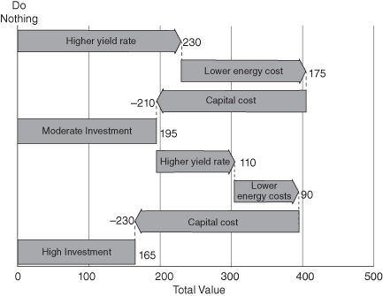
Another form of sources of value analysis that can lead to useful insights is to show the components of the difference in value between two alternatives. For example, suppose that a company is considering upgrading the technology of its production line to improve the yield rate and to lower energy costs. Three alternatives have been identified: (1) do nothing, (2) moderate investment, (3) high investment. Figure 9.5 shows a waterfall chart that depicts how the value changes when going from one alternative to the next. The insight for the decision maker is that in going from Do Nothing (which has zero value) to Moderate Investment, the benefit in higher yield rate and lower energy costs easily outweighs the cost. But in going from Moderate to High Investment, the incremental benefit is not enough to justify the incremental cost, so the net incremental value is negative.
FIGURE 9.5 Waterfall chart of difference in value between alternatives.
A waterfall chart displays value components for a selected strategy, or for the difference between two strategies, very clearly. Sometimes it can be useful to juxtapose value components for all strategies. A value components chart does this (see Fig. 9.6). In it, the value components of each strategy are shown in a pair of vertical stacked bars, where the negatives (investment, opex, taxes, etc.) start at zero in the left bar, and stack downward; and then the positives (revenues, etc.) are in the right bar, starting at the bottom of the negatives and working upward. The net height of the right bar shows the NPV value of the strategy. By juxtaposing all the value components, we enable comparisons across strategies. When these charts have large value components that are similar across strategies, a delta value components chart, which shows the delta of each strategy from a specified reference strategy, can sometimes show the unique characteristics of each strategy more clearly. This gives the equivalent of a waterfall difference chart for all strategies.
FIGURE 9.6 Example value components chart.

The first thing to do with the value components chart is to test the composite perspective it portrays:
- Do we believe the value components for each strategy?
- Do we believe the relative value components across strategies?
- Do we believe the value ranking that emerges from the assessed trade-offs of the objectives?
Next, if value trade-offs are noted, here are some ways to use them to develop an improved strategy:
- Enhance a favorable item.
- Minimize or mitigate an unfavorable item.
- Optimize for a different value measure.
- Find a better compromise among the objectives implicated in the trade-off.
9.8.2 DETERMINISTIC SENSITIVITY ANALYSIS
The purpose of sensitivity analysis is to assess the impact on value of changing each uncertain input across its range of uncertainty. To calculate it, we must collapse all dimensions to a scalar value, normally by using a deterministic value (base case or pseudo EV), taking NPV across time, aggregating business units, and analyzing utility, or financial or MODA value. But it can also sometimes be helpful to look at a specific business unit or objective. The results of sensitivity analysis are displayed in a tornado diagram.
To conduct sensitivity analysis, we need the completed decision model and a set of preliminary ranges of uncertainty on all input variables. Getting the ranges of uncertainty for the sensitivity analysis calls for a careful balancing act. On the one hand, the ranges should represent the considered judgment of the decision-making team. On the other, it would be inappropriate to devote an enormous amount of time and effort to obtain high-quality ranges of uncertainty on the many input factors in a typical decision situation. Assuming the variable definitions have been clearly defined, we spend just a few minutes on assessing the range of uncertainty on each input factor for use in sensitivity analysis. One of the results of the sensitivity analysis is identifying which of the uncertainties really matter to the decision so that much greater attention can then be devoted to refining the ranges of uncertainty on them. In effect, sensitivity analysis is a form of triage in which we use results based on quickly assessed ranges to focus attention on the ranges that merit more careful assessment.
It is crucially important that the ranges of uncertainty used in the sensitivity analysis be defined consistently. The range of uncertainty for each input factor is generally specified by three numbers—low, base, and high. By convention, these are defined as the 10th, 50th, and 90th percentiles, respectively (see Appendix A, Probability). For binary uncertainties, such as events that may or may not occur, the base setting is defined as the more likely state, or in pharmaceuticals or oil and gas, as success. When obtaining these ranges of uncertainty, it is very important to avoid the uncertainty biases identified in Chapter 2. In particular, the anchoring bias should be avoided; appropriately wide ranges of uncertainty should be assessed.
Deterministic sensitivity consists of testing how a value metric varies when each input factor is varied across its range of uncertainty while all other input variables are held at their base or EV settings. Many software packages exist that automate these calculations. The result is a table of sensitivity analysis results and a corresponding tornado diagram. Figure 9.7 shows a typical tornado diagram for a decision alternative. Each tornado bar represents the amount of change in the value metric for an alternative as the input is varied across its range of uncertainty. The input variables are sorted in descending order of the width of the tornado bars so that the most important uncertainties are at the top of the tornado. A tornado diagram can be produced for each value metric of interest for each decision alternative. For example, we see in Figure 9.7 that as we vary the Peak sales input from the low of 500 to the high of 1600, total value varies from −2 to 67. Uncertainty in the Product life input has less of an impact on total value—the range for total value is smaller, going from 15 to 39.
FIGURE 9.7 Example of a tornado diagram.
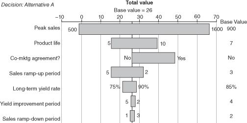
To use a tornado diagram in the value dialogue, compare the large bars to the uncertainties that the decision team thinks should be important, and identify anything additional or missing in the tornado. Check the direction of change in value indicated by each bar against the team’s intuitions. Should value increase or decrease as this input increases? Each point where intuitions differ from the result of the analysis constitutes a “tornado puzzle.” Tornado puzzles are a great way to develop insights or to identify model errors. If a model result seems odd, investigate how it came about and determine whether this makes sense. If it seems wrong, figure out how to improve the model so that it reflects the team’s expertise more closely. If the result holds up, this is an insight for the team. Understand it clearly and explain it to them.
9.8.2.1 Difference Tornado.
One form of tornado diagram that often provides great insight into the decision is the difference (or delta) tornado diagram. This is a tornado diagram showing the impact that uncertainties have on the difference of a value metric between two decision alternatives. If the value metric is the primary (or only) decision criterion, the difference tornado highlights which uncertainties have the power to switch the optimal choice depending on how they turn out. Typically, it is most constructive to investigate the delta between two leading strategies. Figure 9.8 shows an example of a difference tornado diagram.
FIGURE 9.8 Example of a difference tornado diagram.
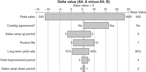
Practitioners accustomed to using only direct tornados for a class of similar problems find them to be of limited use, because “the usual suspects” (e.g., the price of oil in an oil and gas project) are always at the top of the chart. It is frequently the case that these variables affect all strategies roughly equally. In such cases, the impact of the “usual suspects” largely cancels out in a delta tornado, allowing the variables that are important in the decision at hand to rise to the top.
A large bar in a delta tornado diagram that crosses zero (or comes close) indicates that additional information about this variable might cause us to change our decision. Accordingly, it can be worthwhile to convene experts to consider whether there is some way to gather information about any of the leading variables in the delta tornado diagram before the decision must be made.
Some spreadsheet software, such as Microsoft Excel, facilitates the calculation of difference tornados by providing a way to calculate an output seemingly simultaneously for several different settings of the strategy selector input. (In Excel, this feature is called a Data Table.)
Another sort of deterministic sensitivity analysis is to test the impact of two key variables (e.g., the ones from the top of a difference tornado) on the optimal choice. To do this, we set up a table with one variable in the rows and the other in the columns, identify a range of plausible values for each variable, and test which strategy has the best deterministic (base case or pseudo EV) value in each cell of the table. If the strategies are color-coded, this table is called a rainbow chart. This analysis can also be done probabilistically, based on EV values, as illustrated in Section 11.3.5.
9.8.3 SCENARIO ANALYSIS
Just as a strategy is a fixed combination of decision choices, in this handbook, a “scenario” is a fixed combination of uncertainty outcomes. “Scenario Planning” (Kirkwood, 1996) investigates the behavior of a set of strategies under each of a small number of distinct scenarios, where scenarios are also understood to include a chronological story that gives coherence to the set of uncertainty outcomes, and where the scenarios are required to span the plausible range of outcomes for the most important variables. This approach lies on a continuum from no analysis at all to an analysis that considers multiple distinct uncertain factors. Its advantage over analysis with multiple distinct uncertainties is that fewer cases need to be considered. Its disadvantage is that the insights it generates are necessarily less fine-grained, and sometimes less actionable than insights emerging from evaluation with distinct uncertain factors. Accordingly, scenario analysis may help to identify one strategy that seems good, but it is less likely to suggest specific improvements to this strategy. However, scenario analysis can be used to provide insights to help design alternatives or portfolios of alternatives (See Chapter 12) that are robust across all scenarios. The process of analysis is not fundamentally different—just compare cases to identify where value is created, and use this to understand strategies better, and to refine or improve them.
9.9 Deterministic Modeling Using Monetary Multidimensional Value Functions (Approach 1B)
We present in this section a simple illustrative example of a multiple-objective decision analysis that uses a value metric expressed in monetary terms. This is called Approach 1B in the taxonomy of decision analysis practice presented in Chapter 3.
Suppose that an industrial company has a decision to make regarding the level of technology to install in its new manufacturing facility. It has identified three possible alternatives: (1) current technology, (2) state-of-the-art technology, and (3) experimental advanced technology. The company prides itself on being both a financially successful business and a role model in socially responsible behavior. Accordingly, the two objectives for this decision are to maximize the impact on shareholder value (as measured by incremental NPV) and to minimize the environmental damage caused by the manufacturing operations (which in this case is largely in the form of carbon emissions). Deterministic evaluation of the alternatives has produced the results shown in Table 9.1.
TABLE 9.1 Deterministic Results for Manufacturing Technology Example
| Alternative | NPV ($ Million) | 10-Year Carbon Emissions (Million Tons) |
| 1. Current technology | $1500 | 25 |
| 2. State-of-the-art technology | $1300 | 10 |
| 3. Experimental technology | $1000 | 2.5 |
Unfortunately, there is a direct trade-off in these alternatives between incremental NPV and the amount of carbon released, so the best choice is not clear from the results shown in the table. What is needed is a quantitative assessment of the value trade-off between NPV and carbon emissions. After much research, thought, and discussion, the decision makers agree that they are indifferent between increasing NPV by $20 and reducing carbon emissions by 1 ton (and that this trade-off of $20 per ton of carbon is valid for the full range of NPVs and levels of emissions relevant to this decision). This quantified trade-off allows the calculation of an overall value metric, expressed in monetary terms, for comparing the alternatives, as shown in Table 9.2.
TABLE 9.2 Overall Value Metric for Manufacturing Technology Example
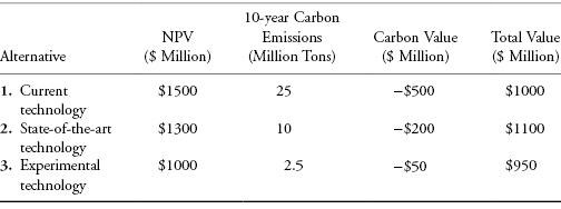
The analysis now leads to the insight that the current technology alternative, which is best in purely financial terms, produces too much carbon to be optimal overall. And the experimental advanced technology alternative, although excellent in reducing carbon emissions, is not quite strong enough financially to be the best choice. So, at least based on deterministic analysis, the alternative with the highest overall value is the State-of-the-art technology. Of course, probabilistic analysis (see Chapter 11) may generate additional insights that could change the ranking of the alternatives.
9.10 Deterministic Modeling Using Nonmonetary Multidimensional Value Functions (Approach 1A)
The preceding section discusses the creation of a monetary value function for multiple objectives (Approach 1B in the taxonomy in Chapter 3). In some private applications and many public applications, it may not be possible or desirable to express all the value measures in monetary terms. In these applications, a nonmonetary value function (Approach 1A) may be used (Keeney & Raiffa, 1976).
For the problem of multiple and, usually, conflicting objectives, value-focused thinking (R. L. Keeney, 1992) recommends focusing first on the values or objectives that the decision is supposed to fulfill, rather than on the alternatives. Using multiple objective decision analysis, we develop a value model, which provides an unbiased, transparent, logical structure to give a numerical overall value for each alternative (see Chapter 3).3 The model is made up of five parts: (1) an objectives or a functional value hierarchy that describes and organizes the objectives (see Chapter 7); (2) value measures that quantify each objective; (3) ranges for each of the value measures, from minimum acceptable (or available) to best possible (or achievable); (4) value functions that describe how value accumulates as one goes from low to high levels in each value measures; and (5) swing weights that specify the relative value of full-range swings in each of the different value measures. The value model must be based on preferences carefully elicited from the decision maker(s) and stakeholders. Value measures can be direct (best) or proxy, and they can be natural (best) or constructed, depending on the time and data available.
9.10.1 THE ADDITIVE VALUE FUNCTION
Multiple objective decision analysis can use any of several mathematical functions to evaluate alternatives. The simplest and most commonly used is the additive value function, which assumes mutual preferential independence (Kirkwood, 1997), which means that the assessment of the value function on one value measure does not depend on the level of the other value measures. For further detail, see Keeney & Raiffa (1976) or Kirkwood (1997). The additive value function uses the following equation to calculate the value of any combination of value measure levels

where for a set of value measure levels given by vector x,
and

(all weights sum to one)
When developing value functions, there are a variety of words used to define the “x-axis” and “y-axis” that describe the value curve.4 In particular, some references use the word “score” to represent the x-axis measure, while others use it to represent the value on the y-axis. To standardize our terminology, we use the term “score” to represent the level of the value measure portrayed on the x-axis (e.g., Car X gets 49 MPG fuel economy ) and “value” to represent our strength of preference for that score on the y-axis (e.g., on a scale of 0–100, fuel economy of 49 MPG is valued at 90).
MODA quantitatively assesses the trade-offs between conflicting objectives by evaluating an alternative’s contribution to the value measures (a score converted to value by single-dimensional value functions) and the importance of each value measure (swing weight). As an important technical note, the swing weights must be on a ratio scale (with an absolute 0), but the value can be on an interval scale or a ratio scale. When interval scales are used for the value functions, 0 value does not necessarily mean no value. Instead, it means the minimum acceptable value on each value measure. Because the same equation in the additive value function applies to all alternatives, no index is required for the alternatives.
9.10.2 SINGLE-DIMENSIONAL VALUE FUNCTIONS
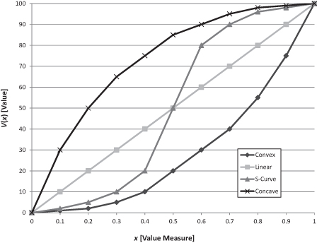
Value functions measure returns to scale on the value measures. They are usually monotonically increasing (decreasing) for value measures aligned with a maximizing (minimizing) objective. The value functions can be discrete or continuous and can have any shape. However, in practice there are four basic shapes: linear, concave, convex, and an S-curve (Fig. 9.9 for increasing value). The linear value function has constant returns to scale: each increment of the measure score is equally valuable. For increasing value measures, the concave value function has decreasing returns to scale: each increment is worth less than the preceding increment. For increasing value measures, the convex value function has increasing returns to scale: each increment of the measure is worth more than the preceding increment. For increasing value measures, the S-curve has increasing, then decreasing, returns to scale on the measure. The S-curve is sometimes used to model leadership goals.
FIGURE 9.9 Four types of value functions for increasing value.
We occasionally see value functions that first rise and then fall (nonmonotonic parabolic shape). This often happens when assessors combine two measures rather than keeping them separate and independent. For example, when assessing the value of the number of bedrooms in a house, we may hear that value increases up to 5 bedrooms, and then starts to decrease. When we ask why, we hear that there are more rooms to clean, air conditioning bills will be higher, and so on. These are legitimate trade-offs, but a better practice is to keep the benefits and costs of the number of rooms as separate value measures.
We have several techniques to assess the value functions using the preferences of experts (the decision makers and/or stakeholders) (Kirkwood, 1997). It is important to note that the experts may or may not be able to directly provide the value functions. In fact, they may not even understand the concept of returns to scale without some discussion and a couple of examples. Being able to explain a value function and help experts assess credible value functions is an important interviewing soft skill. The following are some useful approaches based the authors’ experience.
9.10.3 SWING WEIGHTS
Swing weights play a key role in the additive value model. The most common mistake in MODA is assessing weights without taking into account the specific ranges of value measure scores under consideration. Kirkwood (Kirkwood, 1997) provides a mathematical proof of this statement. The following story has helped many people understand swing weights.
Kirkwood (1997) and Clemen and Reilly (2001) describe swing weight-assessment techniques for individuals. One common way to assess weights from a group of experts is to use voting to obtain ordinal and then cardinal weights:
If disagreements about the weights cannot be resolved, record them. Then do a sensitivity analysis during evaluation to determine if the disagreements are significant. Often, the preferred alternatives are not sensitive to the evaluated weight range. Unfortunately, this weighting technique is not useful for explaining the rationale for the weights assigned. The technique we recommend is the swing weight matrix.
9.10.4 SWING WEIGHT MATRIX
The swing weight matrix8 was designed to help decision makers and stakeholders understand the importance and the impact of the value measure range on the decision. The swing weight matrix defines importance and impact of the range of the value measures in the decision context. The idea of the swing weight matrix is straightforward. A measure that is very important to the decision should be weighted higher than a measure that is less important. A measure that differentiates between alternatives, that is, a measure in which value measure ranges vary widely, is weighted more than a measure that does not differentiate between alternatives. The first step is to create a matrix (Table 9.3) in which the top row defines the value measure importance scale and the left side defines the impact of the range of value measure.9 The levels of importance and variation should be thought of as constructed scales that have sufficient clarity to allow the analyst to uniquely place every value measure in one of the cells. In this example, mission critical is the highest importance, mission enabling is the middle level of importance, and mission enhancing is the lowest level. A measure that is very important to the decision and has a large measure range would go in the upper left of the matrix (cell labeled A). A value measure that has low importance and has small variation in its scale goes in the lower right of the matrix (cell labeled E).
TABLE 9.3 The Elements of the Swing Weight Matrix

9.10.4.1 Consistency Rules.
Since many individuals may participate in the assessment of weights, it is important to insure consistency of the weights assigned. It is easy to understand that a very important measure with a high variation in its range (A) should be weighted more than a very important measure with a medium variation in its range (B1). It is harder to trade off the weights between a very important measure with a low variation in its range (C1) and an important measure with a high variation in its range (B2). Weights should descend in magnitude as we move on the diagonal from the top left to the bottom right of the swing weight matrix. Multiple measures can be placed in the same cell with the same or different weights. If we let the letters represent the diagonals in the matrix A, B, C, D, and E, A is the highest weighted cell, B is the next highest weighted diagonal, then C, then D, and then E. For the swing weights in the cells in Table 9.3 to be consistent, value measure in a given cell must have a greater weight than a value measure in any cell to the right or below the given cell.
9.10.4.2 Assessing Unnormalized Swing Weights.
Once all the value measures are placed in the cells of the matrix, we can use any swing weight technique to obtain the unnormalized weights as long as we follow the consistency rules cited above. In assigning weights, the stakeholders need to assess their trade-offs between importance and impact of the value measure scale. Again, we can use absolute or relative assessments. One absolute assessment technique would be to assign the measure in cell A (the upper left-hand corner cell) an arbitrary large unnormalized swing weight, for example, 100 (fA = 100). Using the value increment approach (Kirkwood, 1997), we can assess the weight of the lowest weighted measure in cell E (the lower right-hand corner) the appropriate swing weight, for example, 1. This means the swing weight of measure A is 100 times more than that of measure E. It is important to consider what the maximum in cell A should be. Common choices are 1000 and 100. Of course, fE can be other numbers besides 1. If we use 100 and 1, we have three orders of magnitude. If we use 1000 and 1, we have four orders of magnitude. Using a value increment approach, unnormalized swing weights can be assigned to all the other value measures relative to fA by descending through the very important measures, then through the important measures, then through the less important measures.
A relative assessment technique for swing weights is the balance beam method (Buede, 2000). This technique uses relative judgments such as “going from the lowest to the highest score on measure 1 is equivalent to going from the lowest to the highest scores on measure 2 and measure 4.” With n – 1 assessments (since the weights must sum to 1), we can solve the set of linear equations for the appropriate swing weights.
9.10.4.3 Calculating Normalized Swing Weights.
We can normalize the weights for the measures to sum to 1 using this equation.
(9.3) 
where fi is the unnormalized swing weight assessed for the ith value measure, i = 1 to n for the number of value measures, and wi are the normalized swing weights from Equation 9.1.
9.10.4.4 Benefits of the Swing Weight Matrix.
We believe this method has six advantages over traditional weighting methods. First, it develops an explicit definition of importance that forces explicit consideration of impact of the measure range. Second, the consistency rules help ensure consistent swing weight assessments. Third, the matrix helps to reduce the number of measures. Suppose cell A has an unnormalized weight of 100 and cell E has an unnormalized weight of 1. It is very obvious that any measure that is placed in cell E will not impact the decision and does not need to be included in the analysis. In practice, this has resulted in significant reduction of the number of value measures. Fourth, it provides a simple yet effective framework to present and justify the weighting preference. Fifth, the approach is very flexible. When measures are added we perform one more assessment for each measure and renormalize. When measures are deleted, all we have to do is renormalize. Finally, swing weights make it easy to communicate a complicated concept to decision makers.
9.10.5 SCORING THE ALTERNATIVES
In this chapter, we assume we know the score of each value measure with certainty. In Chapter 11, we discuss uncertainty analysis. Once we have vetted the quantitative value model and developed alternatives, we must score the alternatives on the value measures. In addition to scoring our alternatives, we should include the current (or baseline) alternative and the ideal (or perfect) alternative. It is important to note that the ideal alternative may not be achievable due to conflicting objectives. Some analysts like to use an operational or realistic ideal as the benchmark. Here, we use the ideal alternative. In practice, the development of the value model and the scoring is an iterative procedure. Many times, the value model has to be revised if scores are not available for a planned value measure or if scorers identify a missing value measure. In fact, to capture this concept, we usually say that “no value model ever survives first contact with the alternatives.10”
A major purpose of value-focused thinking is to generate better alternatives. Therefore, alternative scoring has two purposes: scoring alternatives and generating better ones. The second purpose is often more important! When we begin to score our alternatives, we identify value gaps—chances to improve the alternatives (create better scores) to achieve higher value. Chapter 11 provides more information on improving the alternatives.
There are five primary sources of scores: operational data, test data, simulation, models, and expert opinion. Typically, we will have operational data on the current products and services.
It is prudent to consider who will score the alternatives and how disagreements will be resolved. Four scoring approaches have been particularly successful: performance models, alternative champions, a scoring panel, and alternative champions reviewed by a scoring panel.
9.10.5.1 Scoring by Performance Modeling.
In many decision analysis problems, the modeler scores some alternative value measures by using external performance models. For example, if modeling alternative locations for warehouses, there are so many parameters to consider that it is impossible for a panel to derive a score. Rather, value measures may be scored through simulation model outputs.
9.10.5.2 Scoring by Alternative Champions.
The champion of each alternative scores his or her alternative independent of the others. This approach is useful because it sends information about values from the value function directly to alternative “champions” as they do the scoring. A disadvantage is the perception that a champion of an alternative may bias a score to unduly favor it or that scores from different champions will be inconsistent.
9.10.5.3 Scoring by a Panel.
To avoid the perception of bias and potential inconsistencies, we can use scoring panels. Two types have proven useful. In the first type, we convene a panel of subject matter experts to score and improve the alternatives. Alternative champions present scoring recommendations to the panel, but the panel assigns the final score. In the second type, we have experts score and the champions review the scores. Experts for each value measure score all alternatives being considered (usually with their rationale for the score) and submit it to the analysis team to consolidate. The analysis team then vets the scores with the project champions. The champions usually disagree with something and have a chance to: (1) change the expert’s mind with new data, (2) change the alternative so that it scores better (thereby improving the alternative), or (3) modify when an inconsistency is noticed. We have found virtual panels to be the best approach in large distributed organizations.
9.10.5.4 Scoring by Alternative Champions Reviewed by a Panel.
Having the champion score the alternative and modify it to create more value is the essence of value-focused thinking. A review panel can then ensure the scores are unbiased and consistent.
Once we have scores, we can start evaluating the alternatives—typically through deterministic analysis and uncertainty (or risk) analysis (Chapter 11).
9.10.6 DETERMINISTIC ANALYSIS
Several types of analysis are useful to obtain insights about the alternatives, and many software packages have built-in features to do them. The following analyses will be illustrated in the data center location example.
9.10.6.1 Value Components.
Stacked bar graphs are a useful way to compare alternatives. Usually, the “stacks” show the contribution for each value measure. However, we can plot the stacked bar graphs for any level in the hierarchy. If we do, then analysis usually begins top down to identify insights.
If there are trade-offs of one objective or value component versus another, here are some ways to use them to develop an improved strategy:
- Enhance a favorable item.
- Minimize or mitigate an unfavorable item.
- Optimize for a different value measure.
- Find a better trade-off between the objectives.
9.10.6.2 Value Gaps.
Value gaps are one of the key insights we can extract from value component charts. They are the delta between the best alternative and the ideal alternative for each value measure. We can examine them at all levels in the value hierarchy, so they “shine a light” on areas for value-focused thinking.
9.10.6.3 Value versus Cost.
When using MODA, many decision analysts and decision makers find it useful to separate cost and benefits (value), typically by plotting the value versus the cost of the alternatives. This chart helps decision makers identify the dominant alternatives and enables them to see the value added for the additional cost of the dominant alternatives.
9.10.6.4 Waterfall Chart.
A waterfall chart is a visual depiction of the value contribution between two or more nondominated alternatives.
9.10.6.5 Sensitivity Analysis.
Sensitivity analysis is useful for key parameters, including weights and scores. Performing weights sensitivity analysis can be done using either the assessed weights or the normalized swing weights. In either case, the weights must be normalized over the sensitivity analysis range. The usual assumption is that the weights not subject to sensitivity analysis remain in the same relative proportion. Two sensitivity analysis plots are typical—a rainbow diagram and a tornado diagram
9.11 Illustrative Examples
See Table 1.3 for further information on the illustrative examples. The RNAS example is discussed in Section 9.8. This section illustrates the application of deterministic analysis techniques to the other two examples, Geneptin personalized medicine and the data center location decision. The spreadsheet models for all three examples are available on the Wiley website.
9.11.1 GENEPTIN
The Geneptin team constructed a deterministic financial model in Excel to evaluate the strategic alternatives against the primary objective, ENPV.
The modeling was spearheaded by the decision professional, who interacted with the core team regularly to facilitate team discussions and drive consensus on the strategic alternatives, analysis/evaluation framework, and recommendations on the development strategy.
To determine the proper modeling relationships and help structure model input assumptions, the Geneptin team used an influence diagram to map out the relationships between different parameters (see Fig. 9.10).
FIGURE 9.10 Geneptin influence diagram. 1Decision to develop biomarker will impact all uncertainties shown except Discount Rate. *Probability of Technical and Regulatory Success; ∧Diagnostic. &Profit and loss.

The deterministic model was developed using a cascade of calculations, considering specific personalized medicine-related parameters, such as biomarker prevalence, patient test rate, and so on. DNA Biologics employed influence diagrams to reflect this relationship. Figure 9.11 illustrates a “drill-down” influence diagram for Drug Market Share, showing additional considerations that went into its assessment.
FIGURE 9.11 Geneptin drill-down ID for market share. *Diagnostic; ∧Pricing and Reimbursement.

Based on the deterministic model, sensitivity analysis was done, enabling the team to understand the drivers of value and identify the need to reexamine assumptions that were significant value drivers. The results are shown in a tornado chart for the personalized medicine strategic alternative (see Fig. 9.12).
FIGURE 9.12 Geneptin tornado diagram.

9.11.2 DATA CENTER LOCATION
We illustrate deterministic MODA using the data center location qualitative value model that we describe in Chapter 7. The functional value hierarchy is repeated in Figure 9.13 for ease of reference.
FIGURE 9.13 Data center location functional value hierarchy.

9.11.2.1 Additive Value Model.
As this point we need to determine if we meet the preference independence assumptions of the additive value model (see Chapter 3). We constructed the data center value hierarchy to meet the preferential independence requirements.
9.11.2.2 Decision Analysis Software.
The mathematical calculations shown in this example were done in Excel. For the real problem with 40 measures, we used Logical Decisions (Logical Decisions, Fairfax, VA). INFORMS does a biennial survey of decision analysis software (Buckshaw, 2010) that includes several other decision analysis packages that do MODA. The selection of Excel or a software package depends on several factors including: client preferences, analyst preferences, analyst experience with the packages, funding availability, and time to perform analysis.
9.11.2.3 Value Functions.
We began by working with stakeholders and SMEs to develop value functions for each of the 10 value measures. Note that we had previously developed the range of the x-axis since this was required to assess the swing weights. However, the value functions are not required for the swing weights. The value functions were now developed for each value measure. Table 9.4 summarizes notional data for the value functions that we used in this example. For example, for the function to “provide power for IT and facility,” we identified two objectives: maximize primary power and maximize the potential power growth. For the maximize primary power objective, the value measure was megawatts. The single-dimensional value function for this measure was linear, ranging from 50 to 90 MW. For the maximize potential power growth objective, the value measure was again megawatts and the single-dimensional value function was linear, ranging from 25 to 45 MW. Although this example includes only natural measures, many problems require the development of constructed measures.
TABLE 9.4 Data Center Single-Dimensional Value Functions

9.11.2.4 Swing Weight Matrix.
Once the range has been determined for each value measure, we can assess the swing weights using the swing weight matrix (Section 9.10.4). The art of the swing weight matrix is defining the importance categories (top row) and the impact of the variation (first column) in terms that make sense to the decision makers and the stakeholders. The importance was defined in three categories: critical regional characteristics (e.g., the primary power sources), important site features (e.g., miles from public highway), and features that were fixable with additional funding (e.g., building more floor space or funding longer travel). The impact of site variation was defined in three categories: significant impact (e.g., primary power from 50 to 90 MWs), some impact (e.g., growth power from 25 to 45 MWs), and minor impact (miles from HQ since the facility is designed to be a lights-out facility and the primary travel will be to support the initial equipment installation which are relatively low dollars). Once the value measures are placed in the cells, the unnormalized weights (fi) are assessed with absolute or relative preference judgments. For this study, absolute judgments were used. The normalized weights (wi) are calculated using the equation in Section 9.10.4.
9.11.2.5 Scoring the Alternatives.
In our illustrative example, we assume that eight notional locations passed the screening criteria in Chapter 7 and were scored by the decision team. The scores were obtained from SMEs who were assigned the task of scoring each alternative for each value measures. For example, a power expert determined the current primary power and potential power growth for each site. Table 9.6 lists the alternatives and provides the scores.
9.11.2.6 Single-Dimensional Value Calculations.
Next, we use the scores and the single-dimensional value functions to calculate the single-dimensional value for each alternative for each value measure (Table 9.7). For example, a bandwidth of 9 Gbps has a value of 67 on the linear value function. We used a macro from Kirkwood (Kirkwood, 1997) that does a piecewise linear interpolation between the assessed points on the value function curve. It is important to include the value calculations for the ideal as a check to insure that the value calculations are always 100. The theoretical ideal has value here for verification of the mathematics and can be a guide to improvement of alternatives even if it is not achievable.
9.11.2.7 Normalized Swing Weight Calculations.
Next, we calculate the normalized swing weights. These are the wi columns from Table 9.5. We usually put them in a row in Excel so we can easily do our next calculation. Table 9.8 provides the cell referenced weights and a check to verify that they add to one per Equation 9.2.
TABLE 9.5 Data Center Swing Weight Matrix
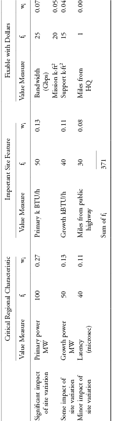
TABLE 9.6 Data Center Scores on Each Value Measure
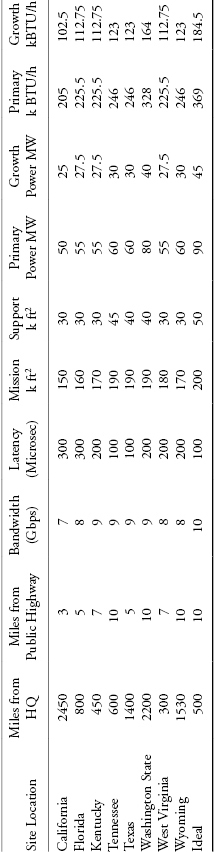
TABLE 9.7 Data Center Single-Dimensional Value Calculations for Each Value Measure
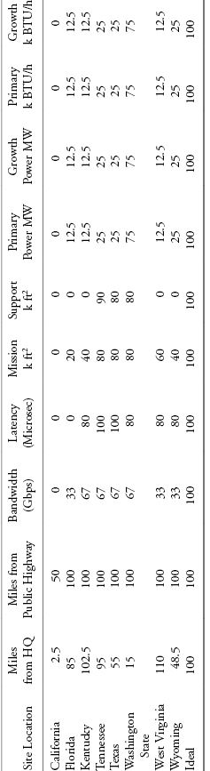
TABLE 9.8 Data Center Normalized Swing Weights

9.11.2.8 Alternative Value Calculations.
The next calculation we need to make is the value calculation for each alternative using the additive value model in Equation 9.1. First, for each alterative, we multiply the swing weight by the value for each measure score. Second, we add up the weighted values for each of the 10 value measures to obtain the total value of each alternative. The results of the first calculation are shown in the first 10 quantitative columns in Table 9.9, and the second calculation is shown in the table’s last column.
TABLE 9.9 Data Center Weighted Value and Total Value Calculations

9.11.2.9 Value Components.
We can use Table 9.9 to plot a stacked bar graph to show the contribution for each value measure. Figure 9.14 shows the data center value components chart for total value. We typically show these charts in color, which makes it easier to differentiate the contributions of each value measure. The Ideal alternative is always shown for reference. The height of each ideal bar is equal to the swing weight × 100. For example the primary power is 27. Although the data are the same as Table 9.9, it is easier to see the contribution of each value measure to the value of each alternative in the chart. Washington State has the highest total value, followed by Tennessee and Texas. Several insights are shown is this chart. First, Washington State scores the best on several value measures, including the highly weighted power (primary power and growth power) and cooling (primary and growth) value measures. The salience of power leads us to ask whether we could create another alternative to capture this benefit, for example, located near cheap power sources (Niagara hydropower, onsite with a minemouth coal-fired plant). The Tennessee and Texas scores are very similar for all the value measures.
FIGURE 9.14 Data center value components chart.
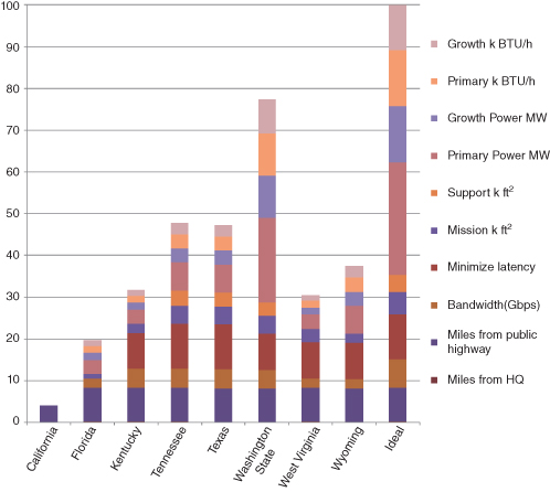
9.11.2.10 Value Gaps.
Value gaps are easy to see from the stacked bar graph. They are the delta between the best alternative and the ideal alternative. An alternative way to plot the value components chart is to show the individual bars for each measure together. The value gaps identify areas where we can attempt to improve the alternatives.
For example, the largest potential value increase for Washington State would be to increase the primary power from 75 to 100 MW. This would increase the value by 6.8 out of 100.
9.11.2.11 Value versus Cost.
Since so many salient benefits were essentially financial, a life cycle cost model was used to evaluate the costs of each site over a common time period. Mathematically, the cost of the alternatives could be one of the objectives and value measures. However, many decision analysts and decision makers find it useful to plot the value versus the cost of the alternatives and look for dominated alternatives. Decision analysts use different costs for different decisions. For example, if the operating and support cost would be about the same for the alternatives the analyst might use the procurement cost. However, for the data center decision, procurement costs will be different, and the operating and support costs of the alternatives depend on several cost factors that depend on the site, for example, the power costs and the security costs. Therefore, for the data center decision, we calculated the life cycle cost (LCC) of each alternative. The life cycle cost factors were land acquisition (purchase or rental), construction/rental of buildings, power, cooling, communications, fire suppression systems, security costs, transportation, and facility and equipment maintenance. Table 9.10 provides the LCC data and the total value of each alternative.
TABLE 9.10 Data Center Life Cycle Cost and Value for Each Alternative
| Life Cycle Cost ($M) | Value | |
| California | 800 | 4.0 |
| Florida | 900 | 19.7 |
| Kentucky | 500 | 31.7 |
| Tennessee | 400 | 47.8 |
| Texas | 600 | 47.3 |
| Washington State | 750 | 77.3 |
| West Virginia | 700 | 30.6 |
| Wyoming | 750 | 37.4 |
| Ideal | 0 | 100.0 |
A plot of this data (Fig. 9.15) helps us quickly identify the dominated alternatives and helps decision makers to see the value added for the additional cost of the dominant alternatives. In our data center problem, we see that Tennessee and Washington State dominate the other alternatives. Assuming that all significant factors are included in the analysis, we would not recommend a dominated alternative since we would be paying more money for less value compared with one of the dominant alternatives. As analysts, we would now focus on analysis of the two nondominated alternatives.
FIGURE 9.15 Data center cost versus value plot. Some analysts reverse the x-axis so best (cheapest) is on the right.

9.11.2.12 Waterfall Chart.
Next, we focus on Washington State and Tennessee. Tennessee has a value of 47.8 and Washington State has a value of 77.3, almost a 30-point increase. A waterfall chart (Fig. 9.16) is a visual depiction of the components of the difference in value between the two nondominated alternatives. Tennessee is better than Washington State for miles from headquarters, latency, and support space. However, Washington State is significantly better than Tennessee for primary power, growth power, primary cooling, and growth cooling. For example, we see a 13.5 point advantage that Washington State has over Tennessee in Primary Power MW. This is calculated from the 50-point difference in values between them (75 for Washington State, 25 for Tennessee) multiplied by the swing weight of Primary Power (0.27)
FIGURE 9.16 Data center waterfall chart.

9.11.2.13 Sensitivity Analysis.
Similar to the difference tornado diagram, we use sensitivity analysis to determine if our preferred alternative is sensitive to a modeling assumption. We can perform sensitivity analysis to any parameter. In MODA, sensitivity analysis can be performed to swing weights, value curve shapes, and scores. The most common sensitivity analysis is to swing weights. When we vary one swing weight, we must decide what changes to make to insure that the swing weights sum to 1. The standard assumption is that the remaining n – 1 swing weights remain in the same proportion. For example, Figure 9.17 shows the sensitivity analysis for the unnormalized swing weight assigned to latency.11 The original latency unnormalized swing weight was 40. In Figure 9.17, we vary the unnormalized swing weight from 0 to 100. Since Washington State has the highest scores in many of the value measures, it is not sensitive to the weight assigned to latency or any other swing weight. In general, the preferred alternative will not be sensitive to the weights.
FIGURE 9.17 Data center sensitivity analysis for latency unnormalized swing weight without change in preferred alternative.
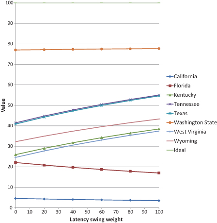
However, suppose we change the following Washington State scores: miles from public highway from 10 to 1, bandwidth from 9 to 7, and latency from 200 to 300. Figure 9.18 shows the sensitivity analysis for the unnormalized swing weight for latency after this change in scores. The preferred data center location is now sensitive to the latency weight. The original latency weight was 40. If the latency weight is less than 70, Washington State is the highest value data center location. However, if the weight is greater than 70, Tennessee is the preferred data center location.
FIGURE 9.18 Data center latency swing weight sensitivity with change in the preferred alternative.

9.11.2.14 Value-Focused Thinking.
Value-focused thinking was used extensively in the data center location problem. The scores and costs presented above were after VFT. The following actions were taken to improve the scores and costs:
- Added higher value alternatives. Initially, there were two alternatives. Several alternatives were added. For example, the Washington alternative was included to get closer to the ideal.
- Negotiated with location owners to provide most favorable features and costs especially on the Tennessee alternative.
- Negotiated with service providers (e.g., local power companies) to obtain the most favorable power capabilities and costs especially on the Tennessee alternative.
9.12 Summary
Our decision analysis approach to evaluating complex alternatives is to develop and refine a composite perspective on how value is created, and to use this to identify even better ways to create value. After eliciting the expertise comprising the composite perspective, the next step is to embody it in a model, and analyze it to facilitate a value dialogue with experts, stakeholders, and decision makers. This chapter presents modeling and deterministic analysis. An influence diagram is an excellent graphical tool to use to identify the variables, the decisions, and their relationships to the value metric. Spreadsheets are a useful platform for decision models. We provide our guidelines for building a spreadsheet decision model and offer suggestions for organizing a spreadsheet model. For financial variables, the P&Ls addressing business units, time and value components should usually be extensively represented. Often decisions and uncertainties should be represented intensively (in strategy table and probabilistic Inputs sheets), enabling subsequent simulation and analysis. For complex models, we need to verify the calculations so we describe approaches for debugging a spreadsheet model. Next, we present important tools for deterministic analysis, including the tornado diagram and difference tornado diagram for deterministic sensitivity analysis and the waterfall chart for displaying the sources of value for an alternative or the differences in value for several alternatives. We present deterministic multiple-objective decision analysis using the most common model, the additive model. We present the mathematics and art of MODA. Finally, we illustrate MODA deterministic modeling and analysis using the data center problem.
KEY TERMS
Notes
1The name pseudo EV is new in this text, but the idea itself is not. We give this slightly pejorative name to the notion out of respect for the discussion in chapter 11 of Flaw of Averages (Savage, 2009). In practice, we find that Savage-style counterexamples are not so common, and we can set up safeguards to ensure that we notice and address them when they do occur. The most important safeguard is never to form a decision based on pseudo EVs unless the insight can be verified using true EV analysis.
2In “scenario planning,” a scenario also carries with it a story about how the ultimate state of affairs came about, and extreme outcomes are of more interest than routine ones. The definition used here is less rich than this view, but not inconsistent with it.
3This section draws on material in Parnell (2007) and Parnell et al. (2011).
4Other terms for v(x) are value score, score, utility, and benefit. Other terms for the score on xi are level, value, attribute, performance, and data.
5The AFT approach is sometimes called “local,” and the VFT approach is sometimes called “global.”
6Approaches similar to DFT are incorporated into several MODA software packages.
7There is some behavioral decision analysis research that demonstrates that relative judgments are easier for experts than absolute judgments.
8The swing weight matrix was developed by Parnell in 2003 and refined by colleagues in the U.S. Army and Innovative Decisions, Inc.
9A 3-by-3 matrix is the most common of a larger (or smaller) number of columns and/or rows may be used for decision with a large number (or small) of value measures. Also, some decision analysts like to put A in the upper right-hand corner.
10The second author coined this phase after the famous military adage—no plan ever survives first contact with the enemy.
11We performed sensitivity analysis to an unnormalized swing weight since this was the judgment that we made and varied the weight from 0 to 100. Some analysts prefer to perform sensitivity analysis to the normalized swing weight and vary the weight from 0 to 1.
REFERENCES
Buckshaw, D. (2010, October). Decision Analysis Software Survey. http://www.informs.org/ORMS-Today/Public-Articles/October-Volume-37-Number-5/Decision-Analysis-Software-Survey, accessed October 20, 2011.
Buede, D. (2000). The Engineering Design of Systems. New York: John Wiley & Sons.
Clemen, R.T. & Reilly, T. (2001). Making Hard Decisions with Decision Tools. Belmont, CA: Duxbury Press.
Dees, R.A., Dabkowski, M.F., & Parnell, G.S. (2010). Decison-focused transformation to improve communications. Decison Analysis, 7(2), 174–182.
Howard, R.A. (1983). The evolution of decision analsysis. In R.A. Howard & J.E. Matheson (eds.), Readings on the Principles and Applications of Decision Analysis, Vols. 1 and 2. Palo Alto, CA: Strategic Decisions Group.
Howard, R.A. & Matheson, J.E. (2005). Influence diagrams. Decision Analysis, 2(3), 127–143.
Keeney, R. & Raiffa, H. (1976). Decision with Mulitiple Objectives: Preference and Value Tradeoffs. New York: John Wiley & Sons.
Keeney, R.L. (1992). Value-Focused Thinking: A Path to Creative Decision Making. Cambridge, MA: Harvard University Press.
Kirkwood, C. (1996). Strategic Decision Making. Belmont, CA: Duxbury Press.
Kirkwood, C. (1997). Strategic Multiple Objective Decision Analysis with Spreadsheets. Belmont, CA: Duxbury Press.
Logical Decisions. (n.d.). http://www.logicaldecisions.com/, accessed October 20, 2011.
Parnell, G.S. (2007). Value-focused thinking. In A. Loerch & L. Rainey (eds.), Methods for Conducting Military Operational Analysis, pp. 619–657. Washington, DC: Military Operations Research Society.
Parnell, G.S., Driscoll, P.J., & Henderson, D.L. (2011). Decision Making for Systems Engineering and Management, 2nd ed. Hoboken, NJ: John Wiley & Sons.
Phillips, L.D. (1984). A theory of requisite decision models. Acta Psychologica, 56, 29–48.
Powell, S.G. & Baker, K.R. (2011). Management Science: The Art of Modeling with Spreadsheets, 3rd ed. Hoboken, NJ: John Wiley & Sons.
Savage, S. (2009). The Flaw of Averages. Hoboken, NJ: John Wiley & Sons.