Appendix A
The Bottom Line
Each of The Bottom Line sections in the chapters suggest exercises to deepen skills and understanding. Sometimes there is only one possible solution, but often you are encouraged to use your skills and creativity to create something that builds on what you know and lets you explore one of many possible solutions.
Chapter 1: The Basics
Find any Civil 3D object with just a few clicks.
By using Prospector to view object data collections, you can minimize the panning and zooming that are part of working in a CAD program. When common subdivisions can have hundreds of parcels or a complex corridor can have dozens of alignments, jumping to the desired one nearly instantly shaves time off everyday tasks.
Master It
Open BasicSite.dwg from www.sybex.com/go/masteringcivil3d2013, and find parcel number 18 without using any AutoCAD commands or scrolling around on the drawing screen. (Hint: Take a look at Figure 1.5.)
Solution
1. In Prospector, expand Sites ⇒ Proposed ⇒ Parcels.
2. Right-click on LOT:18 and select Zoom To.
Modify the drawing scale and default object layers.
Civil 3D understands that the end goal of most drawings is to create hard-copy construction documents. By setting a drawing scale and then setting many sizes in terms of plotted inches or millimeters, Civil 3D removes much of the mental gymnastics that other programs require when you're sizing text and symbols. By setting object layers at a drawing scale, Civil 3D makes uniformity of drawing files easier than ever to accomplish.
Master It
Change the Annotation scale in the model tab of BasicSite.dwg from the 100-scale drawing to a 40-scale drawing. (For metric users: Use BasicSite_METRIC.dwg and change the scale from 1:1000 to 1:500.)
Solution
1. In the lower-right corner of the application window, select 1£ = 40 (1:500) from the Annotation Scale list.
2. Type
REA and press

to regenerate the screen and show the labels at the new scale.
Navigate the Ribbon's contextual tabs.
As with AutoCAD, the Ribbon is the primary interface for accessing Civil 3D commands and features. When you select an AutoCAD Civil 3D object, the Ribbon displays commands and features related to that object. If several object types are selected, the Multiple contextual tab is displayed.
Master It
Continue working in the file BasicSite.dwg (Basic Site_METRIC.dwg). It is not necessary to have completed the previous exercise to continue. Using the Ribbon interface, access the Alignment properties for Road A.
Solution
1. Select the Road A alignment to display the contextual Alignment tab Ribbon.
2. In the Alignment Properties menu, select the Information tab.
3. Click the drop-down list next to the Proposed object style and select Edit Current Selection.
Create a curve tangent to the end of a line.
It's rare that a property stands alone. Often, you must create adjacent properties, easements, or alignments from their legal descriptions.
Master It
Open the drawing MasterIt.dwg (MasterIt_METRIC.dwg). Create a curve tangent to the east end of the line labeled in the drawing. The curve should meet the following specifications:
- Radius: 200.00¢ (60 m)
- Arc Length: 66.580¢ (20 m)
Solution
1. Select Home ⇒ Draw ⇒ Curves ⇒ Create Curve From End Of Object.
2. Select the east side of the line that is labeled “Create a curve tangent to this line.”
3. On the command line, press
to confirm that you will enter a radius value.
4. On the command line, type
200.00 (
60), and then press
5. Type
L to specify the length, and then press
6. Type
66.580 (
20), and then press
Label lines and curves.
Although converting linework to parcels or alignments offers you the most robust labeling and analysis options, basic line- and curve-labeling tools are available when conversion isn't appropriate.
Master It
Add line and curve labels to each entity created in MasterIt.dwg or MasterIt_Metric.dwg. It is recommended you complete the previous exercise so you will have a curve to work with. Choose a label that specifies the bearing and distance for your lines and length, radius, and delta of your curve.
Solution
1. Change to the Annotate tab in the Ribbon.
2. Click the Add Labels button from the Labels & Tables panel.
- Set Feature to Line And Curve.
- Set Label Type to Single Segment.
- Set Line Label Style to Bearing Over Distance.
- Set Curve Label Style to Distance-Radius And Delta.
3. Choose each line and curve.
The default label should be acceptable. If not, perform the following steps:
1. Select a label.
2. From the General Segment Label contextual tab on the Modify panel, click Label Properties.
3. In the resulting AutoCAD Properties dialog, select an alternative label in the General section.
Chapter 2: Survey
Properly collect field data and import it into Civil 3D.
Once survey data has been collected, you will want to pull it into Civil 3D via the Survey Database. This will enable you to create lines and points that correctly reflect your field measurements.
Master It
Create a new drawing based on the template of your choice and a new survey database and import the MASTER_IT_C2.txt (or master_IT_C2_METRIC.txt) file into the drawing. The format of this file is PNEZD (Comma Delimited).
Solution
1. Create a new drawing using a template of your choice.
2. On the Survey tab, create a new local survey database.
3. Create a new network in the newly created survey database.
4. Import the Master_It_C2.txt (or Master_It_C2_METRIC.txt) file and edit the options to insert both the figures and the points.
Set up description key and figure databases.
Proper setup is key to working successfully with the Civil 3D survey functionality.
Master It
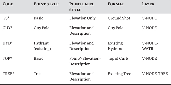
Create a new description key set and the following description keys using the default styles. Make sure all description keys are going to layer V-Node:
Change the description key search order so that the new description key set takes precedence over the default.
Create a figure prefix database called MasterIt containing the following codes:
Solution
1. Open a new drawing based on a Civil 3D template or continue working in the drawing from the previous exercise.
2. OOn the Settings tab, locate the description key area. Right-click Description Key Sets and select New. Give the description key set the name of your choice and click OK.
3. ORight-click the new description key set and select Edit Keys. Add the description keys including the asterisk, as shown in the list.
4. OSet the layer for each item in the table to V-NODE.
5. OClose the description key table and save the drawing.
6. ORight-click Description Key Sets and select Properties.
7. OMove your new description key set to the top of the listing using the arrows. Click OK.
8. OIn the Survey tab, right-click Figure Prefix Databases and select New.
9. OCreate a new figure prefix database called MasterIt.
10. OAdd the required codes to the list. Leave all options as default.
11. Import the file Codetest.txt. When importing, verify that the current figure prefix database is set to MasterIt.
Your file should now contain linework that reflects your efforts.
Translate surveys from assumed coordinates to known coordinates.
Understanding how to manipulate data once it is brought into Civil 3D is important to making your field measurements match your project's coordinate system.
Master It
Create a new drawing and survey database. Start a new drawing based on the template of your choice. Import traverse.fbk (or traverse_METRIC.fbk). Translate the database based on:
- Base Point 1
- Rotation Angle of 10.3053°
Solution
1. Create a new drawing and survey database and import the traverse.fbk (or traverse_METRIC.fbk) file into a network.
2. Using the Translate Survey Network command, rotate the network based on the point number and rotation you were given.
3. Save the drawing and leave it open.
Perform traverse analysis.
Traverse analysis is needed for boundary surveys to check for angular accuracy and closure. Civil 3D will generate the reports that you need to capture these results.
Master It
Use the survey database and network from the previous Master It. Analyze and adjust the traverse using the following criteria:
- Use an Initial Station of value 2 and an Initial Backsight value of 1.
- Use the Compass Rule for Horizontal Adjustment.
- Use the Length Weighted Distribution Method for Vertical Adjustment.
- Use a Horizontal Closure Limit value of 1:25,000.
- Use a Vertical Closure Limit value of 1:25,000.
Solution
1. Continue working in the drawing from the previous Master It. Create a new survey database and network, and import the traverse.fbk (traverse_METRIC.fbk) field book.
2. Create a new traverse from the four points.
3. Perform a traverse analysis on the newly created traverse, and apply the changes to the survey database.
The following files will be generated as a result of the analysis:
- Trav1 Balanced Angles.trv.txt (METRIC_Trav1 Balanced Angles.trv.txt)
- Trav1 Raw Closure.trv.txt (METRIC_Trav1 Raw Closure.trv.txt)
- Trav1 Vertical Adjustment.trv.txt (METRIC_Trav1 Vertical Adjustment.trv.txt)
- Trav1.lso.txt (METRIC_Trav1.lso.txt)
Chapter 3: Points
Import points from a text file using description key matching.
Most engineering offices receive text files containing point data at some time during a project. Description keys provide a way to automatically assign the appropriate styles, layers, and labels to newly imported points.
Master It
Create a new drawing from _AutoCAD Civil 3D (Imperial) NCS.dwt (or _AutoCAD Civil 3D (Metric) NCS.dwt). Revise the Civil 3D description key set to contain only the parameters listed here:
Import the PNEZD (space delimited) file Concord.txt (Concord_METRIC.txt). Confirm that the description keys made the appropriate matches by looking at a handful of points of each type. Do the trees look like trees? Do the hydrants look like hydrants?
Save the resulting file.
Solution
1. Select File ⇒ New, and create a drawing from _AutoCAD Civil 3D (Imperial) NCS Extended.dwt (or _AutoCAD Civil 3D (Metric) NCS.dwt).
2. Switch to the Settings tab of Toolspace, and locate the description key set called Civil 3D.
3. Right-click this set and choose Edit Keys.
4. Delete the first two keys in this set by right-clicking each one and choosing Delete.
5. Revise the remaining key to match the GS specifications listed under the “Master It” instructions.
6. Right-click the GS key, and choose Copy.
7. Create the four additional keys listed in the instructions, and exit Panorama.
8. On the Create Ground Data panel, select Points ⇒ Point Creation Tools and then click the Import Points button on the toolbar.
9. Navigate out to the Concord.txt (Concord_METRIC.txt) file and click Open.
10. Select PNEZD Space Delimited from the listing create a point group with the name of your choosing and click OK.
11. Zoom in to see the points.
12. Save the drawing for use in the next exercise.
Note that each description key parameter (style, label, format, and layer) has been respected. Your hydrants should appear as hydrants on the correct layer, your trees should appear as trees on the correct layer, and so on. Compare your work to EndofChapter_FINISHED.dwg (EndofChapter_METRIC_FINISHED.dwg).
Create a point group.
Building a surface using a point group is a common task. Among other criteria, you may want to filter out any points with zero or negative elevations from your Topo point group.
Master It
Create a new point group called Topo that includes all points except those with elevations of zero or less. Use the DWG created in the previous Master It or start with Master_It.dwg (Master_It_METRIC.dwg).
Solution
1. In Prospector, right-click Point Groups and choose New.
2. On the Information tab, enter Topo as the name of the new point group.
3. Switch to the Exclude tab.
4. Click the Elevation check box to turn it on, and enter <0 in the field.
5. Click OK to close the dialog.
Export points to LandXML and ASCII format.
It's often necessary to export a LandXML or ASCII file of points for stakeout or data-sharing purposes. Unless you want to export every point from your drawing, it's best to create a point group that isolates the desired point collection.
Master It
Create a new point group that includes all the points with a raw description of TOP. Export this point group via LandXML to a PNEZD comma-delimited text file.
Use the DWG created in the previous Master It or start with Master_It.dwg (Master_It_METRIC.dwg).
Solution
1. In Prospector, right-click Point Groups and choose New.
2. On the Information tab, enter Top of Curb as the name of the new point group.
3. Switch to the Include tab.
4. Select the With Raw Descriptions Matching check box, and type TOP in the field.
5. Click OK, and confirm in Prospector that all the points have the description TOP and click OK.
6. Right-click the Top Of Curb point group, and choose Export To LandXML.
7. Click OK in the Export LandXML dialog.
8. Choose a location to save your LandXML file, and then click Save.
9. Navigate out to the LandXML file to confirm it was created.
10. Right-click the Top Of Curb point group, and choose Export Points.
11. Choose the PNEZD comma-delimited format and a destination file, and confirm that the Limit To Points In Point Group check box is selected for the Top of Curb point group. Click OK.
12. Navigate out to the ASCII file to confirm it was created.
13. Save the file Master_It.dwg (Master_It_METRIC.dwg) for use in the next Master It.
Create a point table.
Point tables provide an opportunity to list and study point properties. In addition to basic point tables that list number, elevation, description, and similar options, you can customize point table formats to include user-defined property fields.
Master It
Continue working in Master_It.dwg (Master_It_METRIC.dwg). Create a point table for the Topo point group using the PNEZD format table style.
Solution
1. Change to the Annotate tab, and select Add Tables ⇒ Add Point table.
2. Choose the PNEZD format for the table style.
3. Click Point Groups, and choose the Topo point group.
4. Click OK.
The command line prompts you to choose a location for the upper-left corner of the point table.
5. Choose a location on your screen somewhere to the right of the project.
6. Zoom in, and confirm your point table.
Chapter 4: Surfaces
Create a preliminary surface using freely available data.
Most land development projects involve a surface at some point. During the planning stages, freely available data can give you a good feel for the lay of the land, allowing design exploration before money is spent on fieldwork or aerial topography. Imprecise at best, this free data should never be used as a replacement for final design topography, but it's a great starting point.
Master It
Create a new drawing from the Civil 3D template and set the Coordinate System to NAD83 Connecticut State Plane Zone, US Foot (CT83F) or NAD83 Connecticut State Plane Zone, Meter (CT83). Create a surface named MarlboroughCT_DEM. Add the Marlborough_CT.DEM file (UTM Zone 18, NAD27 datum, meters) downloadable from the book's web page.
Solution
1. In Civil 3D, create a new drawing from the _AutoCAD Civil 3D (Imperial) NCS or _AutoCAD Civil 3D (Metric) NCS template.
2. Change to the Settings tab and right-click the drawing name to open the Drawing Settings dialog.
3. Select an appropriate coordinate system.
4. From the Home tab ⇒ Create Ground Data panel, choose Surfaces ⇒ Create Surface.
5. Set Name to MarlboroughCT_DEM and accept the defaults in the Create Surface dialog, and click OK.
6. Expand the Surfaces ⇒ MarlboroughCT_DEM ⇒ Definition branch.
7. Right-click DEM Files and select the Add option.
8. Use the button to the right of the DEM File Name area to navigate to the Marlborough_CT.dem file and click Open.
9. In the Add DEM File dialog, click the Value column next to CS Code to display the ellipsis button; click that button to display the Select Coordinate Zone dialog.
10. Set the Coordinate System Code to match the DEM file by selecting UTM with NAD27 datum, Zone 18, Meter; Central Meridian 75d W (UTM27-18) and click OK.
11. Click OK in the Add DEM File dialog.
12. Zoom extents to see the surface.
Modify and update a TIN surface.
TIN surface creation is mathematically precise, but sometimes the assumptions behind the equations leave something to be desired. By using the editing tools built into Civil 3D, you can create a more realistic surface model.
Master It
Open the MasteringBoundary.dwg or the MasteringBoundary_METRIC.dwg file. Use the irregular-shaped polyline and apply it to the surface as an outer boundary of the surface.
Solution
1. Draw a polyline that includes the desired area.
2. Expand the Surfaces ⇒ MarlboroughCT_DEM ⇒ Definition branch.
3. Right-click Boundaries and select the Add option.
4. Select the newly created polyline and click Add to complete the boundary addition.
Prepare a slope analysis.
Surface analysis tools allow users to view more than contours and triangles in Civil 3D. Engineers working with nontechnical team members can create strong meaningful analysis displays to convey important site information using the built-in analysis methods in Civil 3D.
Master It
Open the MasteringSlopeAnalysis.dwg or the MasteringSlopeAnalysis_METRIC.dwg file. Create a Slope Banding analysis showing slopes under and over 10 percent and insert a legend to help clarify the image.
Solution
1. Right-click the surface and bring up the Surface Properties dialog.
2. Set the Surface Style field to Slope Banding (2D).
3. Switch to the Analysis tab for the Elevation analysis type.
4. Verify that Create Ranges By is set to Number Of Ranges and that the value is set to 2, and then click the Run Analysis arrow.
5. Change the Maximum Slope for ID 1 and the Minimum Slope for ID 2 both to 10%.
6. Click OK to close the Surface Properties dialog.
7. Select the surface to display the TIN Surface contextual tab.
8. From the TIN Surface contextual tab ⇒ Labels & Tables panel, choose Add Legend Table.
9. Enter
S and then
D at the command line and pick a placement point on the screen to create a dynamic elevations legend.
Label surface contours and spot elevations.
Showing a stack of contours is useless without context. Using the automated labeling tools in Civil 3D, you can create dynamic labels that update and reflect changes to your surface as your design evolves.
Master It
Open the MasteringLabelSurface.dwg or the MasteringLabelSurface_METRIC.dwg file. Label the major contours on the surface at 2¢ and 10¢ (Background) or 1 m and 5 m (Background).
Solution
1. Change the Surface Style to Contours 2′ and 10′ (Background) or Contours 1m and 5m (Background).
2. From the Annotate tab ⇒ Labels & Tables panel, click the Add Labels button
3. Set the Feature to Surface and the Label Type to Contour – Multiple.
4. Set the Major Count Label Style to Existing Major Labels and the Minor Contour Label Style to <none>.
5. Click Add.
6. Pick a point on one side of the site, and draw a contour label line across the entire site.
Import a point cloud into a drawing and create a surface model.
As point cloud data becomes more common and replaces other large-scale data-collection methods, the ability to use this data in Civil 3D is critical. Intensity helps postprocessing software determine the ground cover type. While Civil 3D can't do postprocessing, you can see the intensity as part of the point cloud style.
Master It
Import an LAS format point cloud Denver.las into the Civil 3D template (with a coordinate system) of your choice. As you create the point cloud file, set the style to Elevation Ranges. Use a portion of the file to create a Civil 3D surface model.
Solution
1. Start a new file by using the default Civil 3D template of your choice. Save the file before proceeding as DenverUSA.dwg.
2. In Prospector, right-click the Point Clouds and select the Create Point Cloud option to display the Create Point Cloud wizard.
3. Set the name of the Point Cloud to Denver.
4. Set the Point Cloud Style to Elevation Ranges, and click the Next button.
5. Using the white plus sign to browse to the LAS file.
6. Select Denver.las. Click Finish.
This file contains 4.7 million data points, so be patient while the file imports.
7. Select the bounding box representing the point cloud to display the Point Cloud contextual tab.
8. Select the Add Points To Surface command.
9. Name the surface, set a surface style, and click the Next button.
10. Choose the Window radio button, and click Define Region In Drawing.
11. Define the region by creating a window around the western half of the point cloud.
12. Click Next to see the Summary page and click the Finish button.
Chapter 5: Parcels
Create a boundary parcel from objects.
The first step to any parceling project is to create an outer boundary for the site.
Master It
Open the MasteringParcels.dwg (MasteringParcels_METRIC.dwg) file, which you can download from www.sybex.com/go/masteringcivil3d2013. Convert the line segments in the drawing to a parcel.
Solution
1. From the Home tab's Create Design panel, select Parcel ⇒ Create Parcel From Objects.
2. At the
Select lines, arcs, or polylines to convert into parcels or [Xref]: prompt, pick the lines that represent the site boundary, and press
The Create Parcels – From Objects dialog appears.
3. From the drop-down menus, select Subdivision; Property; and Name, Square Foot & Acres (Name Square Meter & HA) in the Site, Parcel Style, and Area Label Style selection boxes, respectively.
Keep the default values for the remaining options.
4. Click OK to dismiss the dialog.
The boundary polyline forms parcel segments that react with the alignment. The label is placed at the newly created parcel centroid.
Create a right-of-way parcel using the right-of-way tool.
For many projects, the ROW parcel serves as frontage for subdivision parcels. For straightforward sites, the automatic Create ROW tool provides a quick way to create this parcel. A cul-de-sac serves as a terminal point for a cluster of parcels.
Master It
Continue working in the Mastering Parcels.dwg (MasteringParcels_METRIC.dwg) file. Create a ROW parcel that is offset by 25′ (10 m) on either side of the road centerline with 25′ (10 m) fillets at the parcel boundary and alignment ends. Then add the circles representing the cul-de-sac as a parcel.
Solution
1. From the Home tab's Create Design panel, select Parcel ⇒ Create Right Of Way.
2. At the Select parcels: prompt, pick your newly created parcel on screen.
3. Press
to stop picking parcels.
The Create Right Of Way dialog appears.
4. Expand the Create Parcel Right Of Way parameter, and enter 25′ (10 m) in the Offset From Alignment text box.
5. Expand the Cleanup At Parcel Boundaries parameter. Enter 25′ (10 m) in the Fillet Radius At Parcel Boundary Intersections text box.
6. Select Fillet from the drop-down menu in the Cleanup Method selection box.
7. Set the Fillet Radius at Alignment Intersections to 25′ (10 m).
8. Click OK to dismiss the dialog and create the ROW parcels.
9. Trim the two circles at the ROW line to create arcs.
10. From the Home tab's Create Design panel, select Parcel ⇒ Create Parcel From Objects.
11. Pick the two arcs and accept the default settings.
Two new parcels are created.
12. Pick a label at one of the newly created parcels. From the Parcel contextual tab ⇒ Modify panel, select Parcel Layout Tools.
13. Select the Delete Sub-Entity tool and pick the two ROW lines and ROW arc, leaving the outer arc alone.
The cul-de-sac is created and is part of the ROW parcel.
14. Repeat steps 11 and 12 for the other cul-de-sac arc. Press Esc when complete.
Create subdivision lots automatically by layout.
The biggest challenge when creating a subdivision plan is optimizing the number of lots. The precise sizing parcel tools provide a means to automate this process.
Master It
Continue working in the Mastering Parcels.dwg (MasteringParcels_METRIC.dwg) file. Create a series of lots with a minimum of 8,000 sq. ft. (700 m2) and 75′ (20 m) frontage. Set the Use Minimum Offset option to No. Leave all other options at their defaults.
Solution
1. From the Home Tab's Create Design panel, select Parcel ⇒ Parcel Creation Tools.
2. Expand the Parcel Layout Tools toolbar.
3. Change the value of the following parameters by clicking in the Value column and typing in the new values:
- Minimum Area: 8000 Sq. Ft. (700 square meters)
- Minimum Frontage: 75′ (20 m)
4. Change the following parameters by clicking in the Value column and selecting the appropriate option from the drop-down menu:
- Automatic Mode: On
- Remainder Distribution: Redistribute Remainder
5. Click the Slide Line – Create tool.
The Create Parcels – Layout dialog appears.
6. Select Subdivision; Single Family; and Name Square Foot & Acres (Name Square Meter & HA) from the drop-down menus in the Site, Parcel Style, and Area Label Style selection boxes, respectively.
Keep the default values for the rest of the options.
7. Click OK to dismiss the dialog.
8. At the Select Parcel to be subdivided: prompt, pick the Property: 1 label for your property parcel.
9. At the Select start point on frontage: prompt, use your Endpoint osnap to pick the point of curvature on the north end of the project along the ROW parcel segment. The side of the road you start with is up to you.
The parcel jig appears.
10. Move your cursor slowly along the ROW parcel segment, and notice that the parcel jig follows the segment.
11. At the Select end point on frontage: prompt, loop back to the opposite side of the street from where you started. Use your Endpoint osnap to pick the point of curvature along the ROW parcel segment.
12. At the
Specify angle at frontage: prompt, type
90, and press
. If you receive the message
No Solution Found on your command line, try again. This may mean you snapped to the wrong spot.
13. At the
Accept Result: prompt, press
to accept the lot layout.
Note that the parcels are not going to line up properly. For extra credit, fix them to your liking.
Add multiple-parcel segment labels.
Every subdivision plat must be appropriately labeled. You can quickly label parcels with their bearings, distances, direction, and more using the segment labeling tools.
Master It
Continue working in the MasteringParcels.dwg (MasteringParcels_METRIC.dwg) file. Place Bearing Over Distance labels on every parcel line segment and Delta Over Length And Radius labels on every parcel curve segment using the Multiple Segment Labeling tool.
Solution
1. From the Annotate tab, select Add Labels ⇒ Parcels ⇒ Add Parcel Labels.
2. From the drop-down menus, in the Add Labels dialog, select Multiple Segment, Bearing Over Distance, and Delta Over Length And Radius in the Label Type, Line Label Style, and Curve Label Style selection boxes, respectively.
3. Click Add.
4. At the
Select parcel to be labeled by clicking on area label: prompt, pick the area label for each of your single-family parcels. Press
to accept Clockwise as the default.
5. Press Esc to exit the command.
Chapter 6: Alignments
Create an alignment from an object.
Creating alignments based on polylines is a traditional method of building engineering models. With built-in tools for conversion, correction, and alignment reversal, it's easy to use the linework prepared by others to start your design model. These alignments lack the intelligence of crafted alignments, however, and you should use them sparingly.
Master It
Open the MasteringAlignments-Objects.dwg or MasteringAlignments-Objects_METRIC.dwg file, and create alignments from the linework found there with the All Labels label set.
Solution
From the Home tab ⇒ Create Design panel, choose Alignment ⇒ Create Alignment From Objects. Select the lines and arc. Make sure you reverse the alignment if necessary to match the start point indicated in the drawing.
Create a reverse curve that never loses tangency.
Using the alignment layout tools, you can build intelligence into the objects you design. One of the most common errors introduced to engineering designs is curves and lines that aren't tangent, requiring expensive revisions and resubmittals. The free, floating, and fixed components can make smart alignments in a large number of combinations available to solve almost any design problem.
Master It
Open the MasteringAlignments-Reverse.dwg or the MasteringAlignments-Reverse_METRIC.dwg file, and create an alignment from the linework on the right. Create a reverse curve with both radii equal to 200 (or 60 for metric users) and with a pass-through point at the intersection of the two arcs.
Solution
1. From the Home tab ⇒ Create Design panel, choose Alignment ⇒ Alignment Creation Tools.
2. In the Create Alignment – Layout dialog, accept the defaults and click OK to display the Alignment Layout Tools toolbar.
3. Use the Fixed Line (Two Points) tool to trace both lines and press
when complete to end the command.
4. Use the Floating Curve (From Entity, Radius, Through Point) tool to draw an arc from the endpoint of the line with a radius of 200 (or 60 for metric users) to a pass-through point at the intersection of the two sketched arcs.
5. Press
when complete to end the command.
6. Use the Free Curve Fillet (Between Two Entities, Radius) tool to fillet the floating curve created in the previous step and the last fixed segment with a reverse curve with a radius of 200 (or 60 for metric users).
7. Close the Alignment Layout Tools toolbar.
Replace a component of an alignment with another component type.
One of the goals in using a dynamic modeling solution is to find better solutions, not just the first solution. In the layout of alignments, this can mean changing components out along the design path, or changing the way they're defined. The ability of Civil 3D to modify alignments' geometric construction without destroying the object or forcing a new definition lets you experiment without destroying the data already based on an alignment.
Master It
Convert the reverse curve indicated in the MasteringAlignments-Rcurve.dwg or the MasteringAlignments-Rcurve_METRIC.dwg file to a floating arc that is constrained by the next segment. Then change the radius of the curves to 150 (or 45 for metric users).
Solution
1. Select the alignment to activate the contextual tab.
2. From the Alignment contextual tab ⇒ Modify panel, choose Geometry Editor to display the Alignment Layout Tools toolbar.
3. Select the Alignment Grid View tool.
4. Starting with the first segment, click in the Tangency Constraint field and change it to Constrained By Next (Floating).
5. Repeat for the other segments except the last one, which cannot be modified because it is dependent on the previous constraint.
6. Change the radii of the two curves to 150′ (or 45 m for metric users).
Create alignment tables.
Sometimes there is just too much information that is displayed on a drawing, and to make it clearer, tables are used to show bearings and distances for lines, curves, and segments. With their dynamic nature, these tables are kept up to date with any changes.
Master It
Open the MasteringAlignments-Table.dwg or MasteringAlignments-Table_METRIC.dwg file, and generate a line table, a curve table, and a segment table. Use whichever style you want to accomplish this.
Solution
For lines:
1. Select the alignment to activate the contextual tab.
2. From the Alignment contextual tab ⇒ Labels & Tables panel, choose Add Labels ⇒ Alignment ⇒ Multiple Segments and select the alignment.
3. On the Alignment contextual tab ⇒ Labels & Tables panel choose Add Tables ⇒ Add Line.
4. Using the Pick On-Screen button at the bottom of the dialog, select the line segments of the alignment.
If a warning comes up regarding child styles, select the Convert All Selected Label Styles To Tag mode.
5. Click OK to accept the settings in the dialog.
6. Place the table anywhere on your drawing. The bearings and distances are now replaced by tag labels.
For curves:
1. If not done during the lines portion of the exercise, select the alignment and on the Alignment contextual tab ⇒ Labels & Tables panel, choose Add Labels ⇒ Alignment ⇒ Multiple Segments and select the alignment.
2. From the Alignment contextual tab Labels & Tables panel select Add Tables ⇒ Add Curve.
3. Using the Pick On-Screen button at the bottom of the dialog, select the curve segments of the alignment.
4. If a warning comes up regarding child styles, select the Convert All Selected Label Styles To Tag mode.
5. Click OK to accept the settings in the dialog.
6. Place the table anywhere on your drawing. The bearings and distances are now replaced by tag labels.
For segments:
1. If not done during the lines portion of the exercise, select the alignment and on the Alignment contextual tab ⇒ Labels & Tables panel, choose Add Labels ⇒ Alignment ⇒ Multiple Segments and select the alignment.
2. From the Alignment contextual tab ⇒ Labels & Tables panel choose Add Tables ⇒ Add Segment.
3. In the By Alignment section, select the alignment you want to label and click OK.
4. Place the table anywhere on your drawing. The bearings and distances are now replaced by tag labels.
Chapter 7: Profiles and Profile Views
Sample a surface profile with offset samples.
Using surface data to create dynamic sampled profiles is an important advantage of working with a three-dimensional model. Quick viewing of various surface centerlines and grip-editing alignments makes for an effective preliminary planning tool. Combined with offset data to meet review agency requirements, profiles are robust design tools in Civil 3D.
Master It
Open the MasteringProfiles.dwg file (or MasteringProfiles_METRIC.dwg file) and sample the ground surface along Alignment A, along with offset values at 15′ left and 15′ right (or 4.5 m left and 4.5 m right) of the alignment. Generate a profile view showing this information using the Major Grids profile view style with no data band sets.
Solution
1. From the Home tab ⇒ Create Design panel, choose Profile ⇒ Create Surface Profile.
2. Verify that Alignment A and the EG surface are selected and then click the Add button to add the EG surface.
3. Check the Sample Offsets check box and enter 15, -15 (or 4.5, -4.5 for metric users) in the box below the sample offsets and then click the Add button.
4. Click the Draw In Profile button to open the Create Profile View dialog.
5. On the General wizard page, verify that the profile view style is set to Major Grids.
6. On the Data Bands wizard page, verify that Select Band Set is set to _No Bands
7. Click the Create Profile View button.
8. Place the profile anywhere on the drawing.
Lay out a design profile on the basis of a table of data.
Many programs and designers work by creating pairs of station and elevation data. The tools built into Civil 3D let you input this data precisely and quickly.
Master It
In the MasteringProfiles.dwg file (or the MasteringProfiles_METRIC.dwg file), create a layout profile on Alignment A using the Layout profile style and a Complete Label Set with the following information for Imperial users:
| 0+00 |
822.00 |
|
| 1+80 |
825.60 |
300' |
| 6+50 |
800.80 |
|
Or the following information for metric users:
| 0+000 |
250.400 |
|
| 0+062 |
251.640 |
100 m |
| 0+250 |
244.840 |
|
Solution
1. Create a surface profile for Alignment A and generate a profile view (if not done in the previous example) or use the MasteringProfiles_SolutionA.dwg or MasteringProfiles_SolutionA_METRIC.dwg file.
2. From the Home tab ⇒ Create Design panel, choose Profile ⇒ Profile Creation Tools.
3. Select the profile view that shows the surface profile.
4. Verify that Profile Style is set to Layout and Profile Label Set is set to Complete Label Set
5. Click OK to dismiss the Create Profile – Draw New dialog.
6. In the Profile Layout Tools toolbar, set the L-value of the Curve settings to the specified curve length.
7. Use the Draw Tangents With Curves button and the Transparent Commands toolbar to enter station elevation data.
8. If needed, you may move the labels to be legible.
Alternatively, you can import a text file.
Add and modify individual entities in a design profile.
The ability to delete, modify, and edit the individual components of a design profile while maintaining the relationships is an important concept in the 3D modeling world. Tweaking the design allows you to pursue a better solution, not just a working solution.
Master It
In the MasteringProfiles.dwg file (or the MasteringProfiles_METRIC.dwg file) used in the previous exercise, on profile A modify the original curve so that it is 200′ (or 60 m for metric users). Then insert a PVI at Station 4+90, Elevation 794.60 (or at Station 0+150, Elevation 242.840 for metric users) and add a 300′ (or 96 m for metric users) parabolic vertical curve at the newly created PVI.
Solution
1. Using the file from the previous example or MasteringProfiles_SolutionB.dwg or MasteringProfiles_SolutionB_METRIC.dwg file, pick the Design profile, and from the Profile contextual tab ⇒ Modify Profile panel, select the Geometry Editor button.
2. In the Profile Layout Tools toolbar, select the Profile Grid View button.
3. In the Profile Grid View, change the Profile Curve Length field to 200 (or 60 for metric users).
4. In the Profile Layout Tools toolbar, select the Insert PVI button.
5. Using the Profile Station Elevation transparent command, select the profile grid, enter 490 for the station and 794.60 for the elevation (or 150 for the station and 242.840 for the elevation for metric users). Press Esc twice.
6. Back in the Profile Layout Tools toolbar, click the drop-down arrow next to the Vertical Curve Creation button and select More Free Vertical Curves ⇒ Free Vertical Curve (PVI Based).
7. Pick the newly created PVI and enter
300 (or
96 for metric users) for Curve Length. Press
twice.
Apply a standard band set.
Standardization of appearance is one of the major benefits of using styles in labeling. By applying band sets, you can quickly create plot-ready profile views that have the required information for review.
Master It
In the MasteringProfiles.dwg (or the MasteringProfiles_METRIC.dwg) file, apply the Cut and Fill band set to the layout profile created in the previous exercise with the appropriate profiles referenced in each of the bands.
Solution
1. Using the file from the previous example or the MasteringProfiles_SolutionC.dwg or MasteringProfiles_SolutionC_METRIC.dwg file, pick the profile view, and from the Profile View contextual tab ⇒ Modify View panel, choose Profile View Properties to display the Profile View Properties dialog.
2. On the Bands tab, click the Import Band Set, and select the Cut and Fill band set.
3. Select Bottom Of Profile View from the Location drop-down list.
4. Scroll over and change the Profile2 to Layout (1) for both rows.
5. Select Top Of Profile View from the Location drop-down list.
6. Scroll over and change the Profile2 to Layout (1).
Chapter 8: Assemblies and Subassemblies
Create a typical road assembly with lanes, curbs, gutters, and sidewalks.
Most corridors are built to model roads. The most common assembly used in these road corridors is some variation of a typical road section consisting of lanes, curb, gutter, and sidewalk.
Master It
Create a new drawing from the DWT of your choice. Build a symmetric assembly using LaneSuperelevationAOR, UrbanCurbGutterValley2, and LinkWidthAndSlope for terrace and buffer strips adjacent to the UrbanSidewalk. Use widths and slopes of your choosing.
Solution
1. Create a new drawing from the DWT of your choice.
2. From the Home tab ⇒ Create Design panel choose Assembly ⇒ Create Assembly.
3. Name your assembly and set styles as appropriate.
4. Pick a location in your drawing for the assembly.
5. Locate the Lanes tab on the Tool Palettes window.
6. Click the LaneSuperelevationAOR button on the Lanes tab.
7. Use the AutoCAD Properties palette to edit the subassembly parameters, and follow the command-line prompts to set the LaneSuperelevationAOR on the left and right sides of your assembly.
8. Repeat the process with UrbanCurbGutterValley2, LinkWidthAndSlope, and UrbanSidewalk.
9. Complete this portion of the exercise by placing a final LinkWidthAndSlope on the outside of the UrbanSidewalk. (Refer to the “Subassemblies” section of Chapter 8 for additional information.)
10. Save the drawing for use in the next Master It exercise.
Edit an assembly.
Once an assembly has been created, it can be easily edited to reflect a design change. Often, at the beginning of a project you won't know the final lane width. You can build your assembly and corridor model with one lane width, and then change the width and rebuild the model immediately.
Master It
Working in the same drawing, edit the width of each LaneSuperelevationAOR to 14′ (4.3 m), and change the cross slope of each LaneSuperelevationAOR to -3.00%.
Solution
1. Select both lane subassemblies.
Be sure these are the only two elements selected.
2. From the contextual tab ⇒ Modify Subassembly panel choose Subassembly Properties.
3. In the Advanced Parameters, change the width to 14′ (4.3 m).
Note that width will be listed twice. The topmost width reports the default value. You will change the second occurrence.
4. Change the slope to -3.00%.
5. Save the drawing for use in the next Master It exercise.
Add daylighting to a typical road assembly.
Often, the most difficult part of a designer's job is figuring out how to grade the area between the last engineered structure point in the cross section (such as the back of a sidewalk) and existing ground. An extensive catalog of daylighting subassemblies can assist you with this task.
Master It
Working in the same drawing, add the DaylightMinWidth subassembly to both sides of your typical road assembly. Establish a minimum width between the outermost subassembly and the daylight offset of 10′ (3 m).
Solution
1. Locate the Daylight tab on the tool palette.
2. Click the DaylightMinWidth button on the tool palette.
3. Use the AutoCAD Properties palette to verify that Min Width is set to 10'.
4. Follow the command-line prompts to set the DaylightMinWidth on the right side of your assembly.
5. Press Esc on your keyboard to complete the command.
6. Select the right daylight subassembly.
7. From the contextual tab ⇒ Modify Subassembly panel choose Mirror.
8. Click the outermost left point on the LinkWidthAndSlope link.
You should now have daylighting subassemblies visible on both sides of your assembly.
Chapter 9: Custom Subassemblies
Define input and output parameters with default values.
By providing detailed input parameters, you let the Civil 3D user edit your custom subassembly. In addition, by providing detailed output parameters you let them use the subassembly's characteristics to edit the subsequent subassemblies in the assembly.
Master It
Generate a new subassembly PKT file for a subassembly named MasteringLane (or MasteringLaneMetric). For input parameters, define the following:
- Side with a default value of Right
- LaneWidth provided as a decimal precise number with a default value of 12 feet or 3.6 meters
- LaneSlope provided as a percentage with a default value of -3%
- Depth provided as a decimal precise number with a default value of 0.67 feet or 0.2 meters
For output parameters, define the following:
- CalcLaneWidth provided as a decimal precise number
- CalcLaneSlope provided as a percentage
Solution
1. On the Packet Settings tab, set the Subassembly Name to MasteringLane (or MasteringLaneMetric).
2. On the Input/Output Parameters tab, change Default Value for the Side input parameter to Right.
3. Click Create Parameter to add a new parameter for each of the input and output parameters with the following settings (note that the metric values are shown in parentheses if different from the Imperial values):
Define target offsets, target elevations, and/or target surfaces.
Targets allow the subassembly to reference unique items within the drawing. They allow for varying widths, tapered elevations, and daylighting to a surface.
Master It
For the same subassembly from the previous Master It, define an elevation target named TargetLaneElevation with a preview value of -0.33 feet (or -0.1 meters) and an offset target named TargetLaneOffset with a preview value of 14 feet (or 4 meters).
Solution
1. On the Target Parameters tab, click Create Parameter to add a new parameter.
2. Change Name to TargetLaneElevation, verify that Type is set to Elevation, and set Preview Value to -0.33 (or -0.1 for metric).
3. Create another parameter, change Name to TargetLaneOffset, verify that Type is set to Offset, and set Preview Value to 14 (or 4 for metric).
Generate a flowchart of subassembly logic using the elements in the Tool Box.
The Tool Box in Subassembly Composer is full of all sorts of tools. But like a tool box in your garage, the tools are only useful if you know their capabilities and practice using them. The simplest tools are points, links, and shapes, but there are also tools for more complex flow charts.
Master It
Define the subassembly using the width, slope, and depth input parameters defined earlier. Make certain that if the slope of the lane changes based on the targets, then the top and the datum links have matching slopes.
The subassembly should have four points: P1 (“Crown”) located at the origin, P2 (“ETW”) located at the upper-right corner of the lane cross section (with both the TargetLaneElevation and TargetLaneOffset), P3 (“Crown_Subbase”) at the lower left of the lane cross section, and P4 (“ETW_Subbase”) at the lower right of the lane cross section.
The subassembly should have four links: L1 (“Top”, “Pave”) connecting P1 and P2, L2 connecting P1 and P3, L3 (“Datum”, “Subbase”) connecting P3 and P4, and L4 connecting P2 and P4.
The subassembly should have a shape: S1 (“Pave1”).
Solution
1. From the Tool Box ⇒ Geometry branch, drag a Point element (P1) below the Start element.
2. Define point P1 as follows:
A. Set Point Codes to “Crown”.
B. Verify that From Point is set to Origin.
3. From the Tool Box ⇒ Geometry branch, drag a Point element (P2) to below P1.
4. Define point P2 as follows:
A. Set Point Codes to “ETW”.
B. Verify that Type is set to Slope And Delta X.
C. Verify that From Point is set to P1.
D. Set Slope to LaneSlope.
E. Set Delta X to LaneWidth.
F. Set Offset Target (Overrides Delta X) to TargetLaneOffset.
G. Set the Elevation Target (Overrides Slope And Superelevation) to TargetLaneElevation.
H. Verify that the Add Link To From Point check box is selected. This link will automatically be numbered L1.
I. Set the Link ⇒ Codes to “Top”, “Pave”.
5. From the Tool Box ⇒ Geometry branch, drag a Point element (P3) to below P2&L1.
6. Define point P3 as follows:
A. Set Point Codes to “Crown_Subbase”.
B. Verify that Type is set to Delta X and Delta Y.
C. Verify that From Point is set to P1.
D. Set the Delta X to 0.
E. Set the Delta Y to -Depth.
F. Verify that the Add Link To From Point checkbox is selected. This link will automatically be numbered L2.
7. From the Tool Box ⇒ Geometry branch, drag a Point element (P4) to below P3 and L2.
8. Define point P4 as follows:
A. Set Point Codes to “ETW_Subbase”.
B. Verify that Type is set to Delta X and Delta Y.
C. Verify that From Point is set to P2.
D. Set the Delta X to 0.
E. Set the Delta Y to -Depth.
F. Verify that the Add Link To From Point check box is selected. This link will automatically be numbered L3.
G. Change the name for this link to L4.
9. From the Tool Box ⇒ Geometry branch, drag a Link element (automatically numbered L5) to below P4 and L4.
10. Define link currently numbered L5 as follows:
A. Change the Link Number to L3.
B. Set Link Codes to “Datum”, “Subbase”.
C. Verify that Start Point is set to P3.
D. Verify that End Point is set to P4.
11. From the Tool Box ⇒ Geometry branch, drag a Shape element (S1) to below L3.
12. Define shape S1 as follows:
A. Set Shape Codes to “Pave1”.
B. Click the Select Shape In Preview button.
C. Select inside of the closed shape representing the lane.
13. From the Tool Box ⇒ Miscellaneous branch, drag Set Output Parameter to below S1.
14. Define Set Output Parameter as follows:
A. Verify that Output Parameter is set to CalcLaneWidth.
B. Set Value to L1.xlength.
15. From the Tool Box ⇒ Miscellaneous branch, drag Set Output Parameter to below CalcLaneWidth.
16. Define Set Output Parameter as follows:
A. Verify that Output Parameter is set to CalcLaneSlope.
B. Set Value to L1.slope.
Note that there are other ways to define the points and links that will have the same end results.
Import a custom subassembly made with Subassembly Composer into Civil 3D.
A custom subassembly is no good if it is just made and not used. By knowing how to import your PKT file into Civil 3D, you open up the world of building and sharing tool palettes full of subassemblies to help your office's workflow.
Master It
Import your MasteringLane or MasteringLaneMetric subassembly into Civil 3D.
Solution
1. In Subassembly Composer, save your PKT file.
2. Open Civil 3D and create a new drawing using the _AutoCAD Civil 3D (Imperial) NCS or the _AutoCAD Civil 3D (Metric) NCS template.
3. From the Insert tab ⇒ expanded Import panel, choose Import Subassemblies.
4. In the Import Subassemblies dialog, click the folder button to display the Open dialog.
5. Navigate to your PKT file and click Open.
6. Verify that the Import To: Tool Palette check box is selected.
7. Using the drop-down list, either select an existing tool palette or select Create New Palette from the bottom of the list to display the New Tool Palette dialog to define a new palette using the Import Subassemblies dialog
8. Click OK to accept the settings in the Import Subassemblies dialog.
Chapter 10: Basic Corridors
Build a single baseline corridor from an alignment, profile, and assembly.
Corridors are created from the combination of alignments, profiles, and assemblies. Although corridors can be used to model many things, most corridors are used for road design.
Master It
Open the MasteringCorridors.dwg or MasteringCorridors_METRIC.dwg file. Build a corridor named Corridor A on the basis of the Alignment A alignment, the Project Road Finished Ground profile, and the Basic Assembly. Set all frequencies to 10′ (or 3 m for metric users).
Solution
1. From the Home tab ⇒ Create Design panel, choose Corridors.
2. In the Name text box, name your corridor Corridor A.
Keep the default values for Corridor Style and Corridor Layer.
3. Verify that Alignment is set to Alignment A and Profile is set to FG.
4. Verify that Assembly is set to Basic Assembly.
5. Verify that Target Surface is set to the EG surface.
6. Verify that Set Baseline And Region Parameters is checked.
7. Click OK to accept the settings in the Create Corridor dialog, and to display the Baseline And Region Parameters dialog.
8. Click the Set All Frequencies button to display the Frequency To Apply Assemblies dialog.
9. Change the value for all of the frequencies to 10′ (or 3 m for metric users).
10. Click OK to accept the settings in the Frequency To Apply Assemblies dialog.
11. Click OK to accept the settings in the Baseline And Region Parameters dialog.
12. You may receive a dialog warning that the corridor definition has been modified. If you do, select the Rebuild The Corridor option.
Use targets to add lane widening.
Targets are an essential design tool used to manipulate the geometry of the road.
Master It
Open the MasteringCorridorTargets.dwg or MasteringCorridorTargets_METRIC.dwg file. Set Right Lane to target the Alignment A-Left alignment.
Solution
1. From the Corridor contextual tab Modify Corridor panel, choose Corridor Properties.
2. On the Parameters tab, in the Targets column in the baseline row click the ellipsis button to display the Target Mapping dialog.
3. In the Target Mapping dialog, click <None> in the Width Alignment for Right Assembly to display the Set Width Or Offset Target dialog.
4. Select Alignment A-Right and click Add.
5. Click OK to dismiss the Set Width Or Offset Target dialog.
6. Click OK to accept the settings in the Target Mapping dialog box.
7. Click OK to accept the settings in the Corridor Properties and allow the corridor to rebuild.
Create a corridor surface.
The corridor model can be used to build a surface. This corridor surface can then be analyzed and annotated to produce finished road plans.
Master It
Open the MasteringCorridorSurface.dwg or MasteringCorridorSurface_METRIC.dwg file. Create a corridor surface for the Alignment A corridor from Top links. Name the surface Corridor A-Top.
Solution
1. From the Corridor contextual tab ⇒ Modify Corridor panel, choose Corridor Properties.
2. On the Surfaces tab, click the Create A Corridor Surface button in the upper-left corner of the dialog.
3. Click the surface item under the Name column and change the default name of your surface to Corridor A-Top.
4. Verify that Links has been selected from the drop-down list in the Data Type selection box.
5. Verify that Top has been selected from the drop-down list in the Specify Code selection box.
6. Click the Add Surface Item button to add Top Links to the surface definition.
7. Click OK to accept the settings in the dialog; then choose Rebuild The Corridor when prompted.
The corridor and surface will build.
Add an automatic boundary to a corridor surface.
Surfaces can be improved with the addition of a boundary. Single-baseline corridors can take advantage of automatic boundary creation.
Master It
Open the MasteringCorridorBoundary.dwg or MasteringCorridorBoundary_METRIC.dwg file. Use the Automatic Boundary Creation tool to add a boundary using the Daylight code.
Solution
1. Open the Corridor Properties dialog and switch to the Boundaries tab.
2. Right-click on the surface entry and click Add Automatically ⇒ Daylight.
3. Click OK to accept the settings in the dialog; then choose Rebuild The Corridor when prompted.
The corridor and surface will build.
Chapter 11: Advanced Corridors, Intersections, and Roundabouts
Create corridors with noncenterline baselines.
Although for simple corridors you may think of a baseline as a road centerline, other elements of a road design can be used as a baseline. In the case of a cul-de-sac, the EOP, the top of curb, or any other appropriate feature can be converted to an alignment and profile and used as a baseline.
Master It
Open the MasteringAdvancedCorridors.dwg (MasteringAdvancedCorridors_METRIC.dwg) file, which you can download from www.sybex.com/go/masteringcivil3d2013. Add the cul-de-sac alignment and profile to the corridor as a baseline. Create a region under this baseline that applies the Intersection Typical assembly.
Solution
1. Select the corridor, right-click, and choose Corridor Properties.
2. Switch to the Parameters tab.
3. Click Add Baseline, choose Cul de Sac EOP in the Create Corridor Baseline dialog, and click OK.
4. In the Profile column, click inside the <Click here…> box, choose Cul de Sac EOP FG in the Select A Profile dialog, and click OK.
5. Right-click the new baseline, and choose Add Region.
6. Select Intersection Typical in the Create Corridor Region dialog.
7. Click OK to leave the Corridor Properties dialog and rebuild the corridor.
Add alignment and profile targets to a region for a cul-de-sac.
Adding a baseline isn't always enough. Some corridor models require the use of targets. In the case of a cul-de-sac, the lane elevations are often driven by the cul-de-sac centerline alignment and profile.
Master It
Continue working in the Mastering Advanced Corridors.dwg (Mastering Advanced Corridors_METRIC.dwg) file. Add the Second Road alignment and Second Road FG profile as targets to the cul-de-sac region. Adjust Assembly Application Frequency to 5′ (1 m), and make sure the corridor samples are profile PVIs.
Solution
1. Select the corridor. From the Corridor contextual tab Modify Corridor panel, click Corridor Properties.
2. Switch to the Parameters tab.
3. Click the Target Mapping button in the Cul de Sac EOP region.
4. In the Target Mapping dialog, assign Second Road as Width Alignment for Lane - L and Second Road FG profile as Outside Elevation Profile; then click OK.
5. Click OK to leave the Target Mapping dialog.
6. Click the Frequency button in the appropriate region.
7. Change the Along Curves value to 5′ (1 m) and the At Profile High/Low Point value to Yes.
8. Click OK to exit the Frequency To Apply To Assemblies dialog.
9. Click OK to leave the Corridor Properties dialog and rebuild the corridor.
Create a surface from a corridor and add a boundary.
Every good surface needs a boundary to prevent bad triangulation. Bad triangulation creates inaccurate contours, and can throw off volume calculations later in the process. Civil 3D provides several tools for creating corridor surface boundaries, including an Interactive Boundary tool.
Master It
Continue working in the Mastering Advanced Corridors.dwg (Mastering Advanced Corridors_METRIC.dwg) file. Create an interactive corridor surface boundary for the entire corridor model.
Solution
1. Select the corridor. From the Corridor contextual tab ⇒ Modify Corridor panel, click Corridor Properties.
2. Switch to the Boundaries tab.
3. Select the corridor surface, right-click, and choose Add Interactively.
4. Follow the command-line prompts to add a feature line–based boundary all the way around the entire corridor.
5. Press C to close the boundary, and then press
to end the command.
6. Click OK to leave the Corridor Properties dialog and build the corridor.
An example of the finished exercise can be found in Mastering Advanced Corridors Finished.dwg (Mastering Advanced Corridors_METRIC.dwg) at the book's web page.
Chapter 12: Superelevation
Add superelevation to an alignment.
Civil 3D has convenient and flexible tools that will apply safe, correct superelevation to an alignment curve.
Master It
Open the Master Super.dwg (Master Super_METRIC.dwg) file, which you can download from www.sybex.com/go/masteringcivil3d2013. Set the design speed of the road to 20 miles per hour (35 km per hour) and apply superelevation to the entire length of the alignment. Use AASHTO 2004 Design Criteria with an eMax of 6% 2-Lane.
Solution
1. Select the alignment. From the Alignment contextual tab ⇒ Modify panel, choose Alignment Properties.
2. On the Design Criteria tab, place a check mark next to Use Criteria Based Design.
3. Set the design criteria file and superelevation eMax from the right side of the dialog.
4. Set the design speed to 20 mph (35 kmph) on the left side, and click OK.
5. From the contextual tab, click Superelevation ⇒ Calculate/Edit Superelevation.
6. Click Calculate Superelevation Now.
7. Step through the superelevation wizard, taking all the defaults for pivot and shoulder control.
8. On the Attainment page, place a check mark next to Automatically Resolve Overlap. Click Finish.
You should now have superelevation applied to the design with no overlap.
Create a superelevation assembly.
In order for superelevation to happen, you need to have an assembly that is capable of superelevating.
Master It
Continue working in Master Super.dwg (Master Super_METRIC.dwg). Create an assembly similar to the one in the top image of Figure 12.11. Set each lane to be 14′ (4.5 m) wide, and each shoulder to be 6′ (2 m) wide. Leave all other options at their defaults. If time permits, build a corridor based on the alignment and assembly.
Solution
1. From the Home tab ⇒ Create Design panel ⇒ Assembly, choose Create Assembly.
2. Name the assembly AOR and set the assembly type to Undivided Crowned Road. Click OK.
3. Click to place the assembly in the graphic.
4. From the Lanes palette, click the LaneSuperelevationAOR subassembly.
5. Click the assembly to place one lane on the right; click again to place the assembly to the left.
6. Select the right subassembly and set its Use Superelevation parameter to Right Lane Outside.
7. Select the left subassembly and set its Use Superelevation parameter to Left Lane Outside.
8. Place the shoulders on each side.
9. If time permits, create a corridor based on the alignment and assembly you just created.
10. Save the drawing.
Create a rail corridor with cant.
Cant tools are new to Civil 3D 2013 and allow users to create corridors that meet design criteria specific to rail needs.
Master It
In the drawing MasterCant.dwg (MasterCant_METRIC.dwg), create a Railway assembly with the RailSingle subassembly using the default parameters for width and depth. Add a LinkSlopetoSurface generic link with 50% slope to each side. Add cant to the alignment in the drawing using the default settings for attainment. Create a corridor from these pieces.
Solution
1. From the Home tab ⇒ Create Design panel ⇒ Assembly, choose Create Assembly.
2. Name the assembly Rail and set the type to Railway.
3. From the Bridge And Rail palette, click the rail single subassembly.
4. Click the assembly in the drawing to place the rail design.
5. From the Generic palette, click LinkSlopetoSurface.
6. Set the slope to –50% and click once on each side of the assembly to place the link.
7. Press Esc to complete the process.
8. Select the alignment. From the alignment contextual tab ⇒ Modify panel, click Cant ⇒ Calculate/Edit Cant.
9. Click Calculate Cant Now, and click Finish.
10. Build a corridor from the alignment, assembly, and the proposed profile (which has been designed for you ahead of time).
If you need assistance building your corridor, review Chapters 10 and 11. But hopefully you've figured it out by this point!
Create a superelevation view.
Superelevation views are a great place to get a handle on what is going on in your roadway design. You can visually check the geometry as well as make changes to the design.
Master It
Open the drawing MasterView.dwg (MasterView_METRIC.dwg). Create a superelevation view for the alignment. Show only the Left and Right Outside Lanes as blue and red, respectively.
Solution
1. Select the alignment and choose Superelevation ⇒ Create Superelevation View.
2. In the Create Superelevation View dialog, toggle off Left Outside Shoulder and Right Outside Shoulder. The remaining check boxes will be for the lane views.
3. Set Left Outside Lane Color to Blue, set Right Outside Shoulder Color to Red, and click OK.
4. Place the view in the drawing.
Chapter 13: Cross Sections and Mass Haul
Create sample lines.
Before any section views can be displayed, sections must be created from sample lines.
Master It
Open MasterSections.dwg (MasterSections_METRIC.dwg) and create sample lines along the USH 10 alignment every 50′ (20 m). Set the left and right swath widths to 50′ (20 m).
Solution
1. From the Home tab ⇒ Profile & Section Views, click Sample Lines.
2. Select the USH_10 alignment and sample all data.
3. In the Sample Line tools, select the By Range Of Station option.
4. Create sample lines by station range and set your sample line distance to
50′ (
20 m); then click OK and
to complete the command.
Create section views.
Just as profiles can only be shown in profile views, sections require section views to display. Section views can be plotted individually or all at once. You can even set them up to be broken up into sheets.
Master It
In the previous exercise, you created sample lines. In that same drawing, create section views for all the sample lines. Use all the default settings and styles.
Solution
1. Continue working in MasterSections.dwg (MasterSections_METRIC.dwg).
2. Select one of the sample lines.
3. From the Sample Line contextual tab, click Create Section View ⇒ Create Multiple Section Views.
4. Leave all options at their defaults, and click Create Section Views.
5. Click in the graphic to place the views.
Define and compute materials.
Materials are required to be defined before any quantities can be displayed. You learned that materials can be defined from surfaces or from corridor shapes. Corridors must exist for shape selection, and surfaces must already be created for comparison in materials lists.
Master It
Using MasterSections.dwg (MasterSections_METRIC.dwg), create a materials list that compares Existing Intersection with HWY 10 DATUM Surface. Use the Earthworks Quantity takeoff criteria.
Solution
1. Continue working in MasterSections.dwg (MasterSections_METRIC.dwg).
2. Select one of the sample lines.
3. From the Sample Lines contextual tab ⇒ Launch Pad panel, click Compute Materials. Select the alignment and sample line group, and then click OK.
4. Set the quantity takeoff criteria to Earthworks.
5. Set the existing ground surface to Existing Intersection.
6. Set the datum to HWY 10 DATUM, and click OK.
Graphically nothing will appear. Continue to the Master It to see the results of your work.
Generate volume reports.
Volume reports give you numbers that can be used for cost estimating on any given project. Typically, construction companies calculate their own quantities, but developers often want to know approximate volumes for budgeting purposes.
Master It
Continue using MasterSections.dwg (MasterSections_METRIC.dwg. Use the materials list created earlier to generate a volume report. Create a web browser–based report and a Total Volume table that can be displayed on the drawing.
Solution
1. Continue working in MasterSections.dwg (MasterSections_METRIC.dwg).
2. Without any object selected, select Analyze ⇒ Volumes And Materials panel, and click Volume Report.
3. Leave all options at their defaults, and click OK.
4. If asked “Do you want to allow scripts to run?” click Yes.
Your report will display.
5. Close the browser window.
6. In Civil 3D, select Analyze ⇒ Volumes And Materials panel, and click Total Volume Table.
7. Leave all options at their defaults and click OK.
Chapter 14: Pipe Networks
Create a pipe network by layout.
After you've created a parts list for your pipe network, the first step toward finalizing the design is to use Pipe Network By Layout.
Master It
Open the MasteringPipes.dwg or Mastering pipes_METRIC.dwg file. From the Home tab ⇒ Create Design panel ⇒ Pipe Network, select Pipe Network Creation Tools to create a sanitary sewer pipe network. Use the Composite surface, and name only structure and pipe label styles. Don't choose an alignment at this time. Create 8″ (200 mm) PVC pipes and concentric manholes. There are blocks in the drawing to assist you in placing manholes. Begin at the START HERE marker, and place a manhole at each marker location. You can erase the markers when you've finished.
Solution
1. From the Home tab's Create Design panel, select Pipe Network ⇒ Pipe Network Creation Tools.
2. In the Create Pipe Network dialog, set the following parameters:
- Network Name: Mastering
- Network Parts List: Sanitary Sewer
- Surface Name: Corridor FG
- Alignment Name: <none>
- Structure Label Style: Name Only (Sanitary)
- Pipe Label Style: Name Only
3. Click OK. The Pipe Layout Tools toolbar appears.
4. Set the structure to SMH and the pipe to 8 Inch PVC (200 mm PVC).
5. Click Draw Pipes And Structures, and use your Insertion Osnap to place a structure at each marker location.
6. Press
to exit the command.
7. Move the structure labels.
8. Select a marker, right-click, choose Select Similar, and click Delete.
Create an alignment from network parts and draw parts in profile view.
Once your pipe network has been created in plan view, you'll typically add the parts to a profile view based on either the road centerline or the pipe centerline.
Master It
Continue working in the MasteringPipes.dwg (Mastering pipes_METRIC.dwg) file. Create an alignment from your pipes so that station zero is located at the START HERE structure. Create a profile view from this alignment, and draw the pipes on the profile view.
Solution
1. Select the structure labeled START HERE to display the Pipe Networks contextual tab and select Alignment From Network on the Launch Pad panel.
2. Select the last structure in the pipe run, and press
to accept the selection.
3. In the Create Alignment dialog, name the alignment Mastering and make sure the Create Profile And Profile View check box is selected.
4. Accept the other defaults, and click OK.
5. In the Create Profile dialog, sample both the EG and Corridor FG surfaces for the profile.
6. Click Draw In Profile View.
7. In the Create Profile View dialog, click Create Profile View and choose a location in the drawing for the profile view.
A profile view showing your pipes appears.
Label a pipe network in plan and profile.
Designing your pipe network is only half of the process. Engineering plans must be properly annotated.
Master It
Continue working in the MasteringPipes.dwg (Mastering pipes_METRIC.dwg) file. Add the Length Description And Slope style label to profile pipes and the Data With Connected Pipes (Sanitary) style to profile structures. Add the alignment created in the previous Master It to all pipes and structures.
Solution
1. Select one of the pipe or structure objects. From the Pipe Networks contextual tab, select Add Pipe Network Labels.
2. In the Add Labels dialog, change Feature to Pipe Network, and then change Label Type to Entire Network Profile.
- For pipe labels, choose Length Description And Slope.
- For structure labels, choose Data With Connected Pipes (Sanitary).
3. Click Add, and choose any pipe or structure in your profile view.
4. Drag or adjust any profile labels as desired.
5. In the Prospector tab of Toolspace, expand Pipe Networks ⇒ Networks ⇒ Mastering and select Pipes.
6. Select all pipes in Prospector, right-click on Reference Alignment column header, and select Edit.
7. Choose the Mastering alignment.
8. Repeat steps 6 and 7 but choose Structures.
Create a dynamic pipe table.
It's common for municipalities and contractors to request a pipe or structure table for cost estimates or to make it easier to understand a busy plan.
Master It
Continue working in the MasteringPipes.dwg (Mastering pipes_METRIC.dwg) file. Create a pipe table for all pipes in your network. Use the default table style.
Solution
1. Select one of the pipe or structure objects. From the Pipe Networks contextual tab ⇒ Add Tables ⇒ Add Pipe.
2. In the Pipe Table Creation dialog, make sure your pipe network is selected.
3. Accept the other defaults, and click OK.
4. Place the table in your drawing.
Chapter 15: Storm and Sanitary Analysis
Create a catchment object.
Catchment objects are the newest object type that Civil 3D can use to determine the area and time of concentration of a site. You can create a catchment from a surface, but in most cases you will use the option to create from polyline.
Master It
Create a catchment for predeveloped conditions on the site.
Solution
1. Open the file Mastering Catchment Creation.dwg (or Mastering Catchment Creation_METRIC.dwg).
2. On the Analyze tab, choose Catchments ⇒ Create Catchment Group.
3. Name the new catchment group Predeveloped and click OK.
4. On the Analyze tab, select Catchments ⇒ Create Catchment From Object.
5. Select the red closed polyline that represents the catchment.
6. When prompted for the flow path, select the dashed polyline that runs through the site. Be sure to select it on the north part of the site (the uphill side).
7. In the Create Catchment dialog, name the catchment Basin A.
8. Leave all other styles and settings at their defaults and click OK.
You now have a completed catchment.
9. Press Esc when complete.
Export pipe data from Civil 3D into SSA.
Civil 3D by itself cannot do pipe flow or runoff calculations. For this reason, it is important to export Civil 3D pipe networks into the Storm And Sanitary Analysis portion of the product.
Master It
Verify your pipe export settings and then export to SSA.
Solution
1. Open Export to SSA.dwg (or Export to SSA_METRIC.dwg).
2. Select the Settings tab of Toolspace; then expand Pipe Networks and expand Commands.
3. Double-click the EditInSSA option.
4. Expand the Storm Sewers Migration Defaults area.
5. Click the field for part matching defaults.
6. Click the ellipsis to open the Part Matchup Settings dialog.
7. Examine the Import tab and verify that the settings make sense.
8. Switch to the Export tab and examine your options for bringing files back into Civil 3D.
9. Click OK — no changes are needed.
10. Click OK to exit the command settings.
11. Switch to the Analyze tab in Civil 3D.
12. Click Edit In Storm And Sanitary Analysis.
13. Click OK to export the Highway Drainage storm network.
14. When Storm Sewers launches, click OK to create a new project.
15. Click No to saving the log file.
16. Switch to the Plan View tab.
17. Double-click one of the structures. Make sure it contains elevation data.
18. Save the SSA file and exit.
Export a stage-storage table from Civil 3D.
When designing detention basins in Civil 3D, you will often need to export surface data for analysis in SSA.
Master It
Generate a stage storage table for a detention basin surface. Determine how much water the pond can hold.
Solution
1. In Civil 3D, open Master_It_Pond.dwg (or Master_It_Pond_METRIC.dwg).
2. Select the surface in the drawing.
3. From the Analyze flyout panel of the context tab, select Stage Storage.
4. From the Stage Storage dialog, click Define Basin.
5. On the Define Basin From Entities dialog, name the basin New Pond. Click Define.
6. When prompted, select the surface from the graphic.
You should be returned to the Stage Storage dialog.
7. Make note of the maximum storage of the pond.
Your result should be 346,489.16 cubic feet (9,670.99 cubic meters).
8. Click Save Table.
9. Save the table as New Pond.AeccSST.
10. Close the Stage Storage dialog by clicking Cancel.
11. Save and close the drawing.
Model drainage systems in SSA.
SSA is capable of modeling everything from complex drainage systems to simple culverts.
Master It
Determine which links flood during a 2-hour, 50-year storm event. Model the example drainage design using SSA.
Solution
1. In SSA, open Master_It_Storm.spf (or Master_It_Storm_METRIC.spf).
2. Right-click Subbasin 1 and select Connect To. Connect Subbasin 1 to Inlet 9-W.
3. Repeat step 2 for the three remaining subbasins.
The subbasins drain to the following inlets:
- Subbasin 2 drains to Inlet 2-E.
- Subbasin 3 drains to Inlet 7-W.
- Subbasin 4 drains to Inlet 3-E.
4. Double-click Analysis Options.
5. On the General tab, set the storm duration to 2 hours.
6. On the Storm Selection tab, choose a single 50-year storm. Click OK when complete.
7. Click Run Analysis.
At the end of the process, the analysis will show C&G 2 and C&G 4 as flooded.
Chapter 16: Grading
Convert existing linework into feature lines.
Many site features are drawn initially as simple linework for the 2D plan. By converting this linework to feature line information, you avoid a large amount of rework. Additionally, the conversion process offers the ability to drape feature lines along a surface, making further grading use easier.
Master It
Open the MasteringGrading.dwg or MasteringGrading_METRIC.dwg file from the book's web page. Convert the magenta polyline, describing a proposed temporary swale, into a feature line and drape it across the EG surface to set elevations, and set intermediate grade break points.
Solution
1. From the Home tab ⇒ Create Design panel, choose Feature Lines ⇒ Create Feature Lines From Objects.
2. Select the polyline.
3. Toggle the Assign Elevations check box on and then click OK.
4. Select the EG surface in the Assign Elevations dialog.
5. Verify that Insert Intermediate Grade Break Points is selected.
6. Click OK to close the dialog and return to your model.
Model a simple linear grading with a feature line.
Feature lines define linear slope connections. This can be the flow of a drainage channel, the outline of a building pad, or the back of a street curb. These linear relationships can help define grading in a model, or simply allow for better understanding of design intent.
Master It
Edit the curve on the feature line you just created to be 100′ (30 m). Set the grade from the west end of the feature line to the next PI to 4 percent, and the remainder to a constant slope to be determined in the drawing. Draw a temporary profile view to verify the channel is below grade for most of its length.
Solution
1. Select the feature line to activate the Feature Line contextual tab.
2. From the Feature Line contextual tab ⇒ Modify panel, toggle on the Edit Geometry panel if not already visible.
3. From the Feature Line contextual tab ⇒ Edit Geometry panel, choose the Edit Curve tool.
4. Select the feature line curve.
5. In the Edit Feature Line Curve dialog, change the radius to 100′ (30 m) and click OK.
6. Press
to end the command.
7. From the Feature Line contextual tab ⇒ Modify panel, toggle on the Edit Elevations panel if not already visible.
8. From the Feature Line contextual tab ⇒ Edit Elevations panel, choose the Set Grade/Slope Between Two Points tool.
9. Use the End Osnap to pick the western end of the feature line, and press
to accept the elevation.
10. Select the next PI at the start of the curve.
11. At the
Specify grade or [SLope Elevation Difference SUrface Transition]: prompt, enter
4 to set the grade.
12. Select the feature line again.
13. Pick the PI at the start of the curve, and press
to accept the elevation.
14. Pick the PI at the upstream (eastern) end of the channel, and press
to accept the grade.
15. Press
to end the command.
16. Select the feature line, and from the Feature Line contextual tab ⇒ Launch Pad panel, choose Quick Profile.
17. Click OK to accept the defaults and pick a point on the screen to draw the quick profile view.
18. Dismiss Panorama to view the Quick Profile.
Model planar site features with grading groups.
Once a feature line defines a linear feature, gradings collected in grading groups model the lateral projections from that line to other points in space. These projections combine to model a site much like a TIN surface, resulting in a dynamic design tool that works in the Civil 3D environment.
Master It
Use the two grading criteria to define the pilot channel, with grading on both sides of the sketched centerline. Define the channel using a Grading to Distance of 5′ (1.5 m) with a slope of 3:1 and connect the channel to the EG surface using a grading with slopes that are 4:1. Generate a surface from the grading group. If prompted, do not weed the feature line.
Solution
1. From the Home tab ⇒ Create Design panel, choose Grading ⇒ Grading Creation Tools to activate the Grading Creation Tools toolbar.
2. Click the Create A Grading Group tool to create a grading group.
3. Verify that the Automatic Surface Creation option is checked, and click OK.
4. Click OK to accept the surface creation options.
5. Click the Set The Target Surface tool to set the target surface to EG, and click OK.
6. Change Grading Criteria to Grade To Distance.
7. Click the Create Grading tool, and pick the feature line.
8. If the Weed Feature Line dialog appears, select Continue Grading Without Feature Line Weeding
9. Pick the left or right side, and press
to model the full length.
10. Enter 5′ (1.5 m) for the distance.
11. Press
to accept entering the slope.
12. Enter 3 for the slope value.
13. Pick the main feature line again, and grade the other side using the same steps.
14. Change Grading Criteria to Grade To Surface, and then create a grading object on both the left and right sides with slopes of 4:1.
15. Press Esc to complete the gradings.
Chapter 17: Plan Production
Create view frames.
When you create view frames, you must select the template file that contains the layout tabs that will be used as the basis for your sheets. This template must contain predefined viewports. You can define these viewports with extra vertices so you can change their shape after the sheets have been created.
Master It
Open the MasteringPlanProduction.dwg or MasteringPlanProduction_METRIC.dwg file. Run the Create View Frames wizard to create view frames for Alignment A in the current drawing. (Accept the defaults for all other values.) These view frames will be used to generate Plan and Profile sheets on ARCH D (ISO A1) sheets at 20 scale (1:200 scale) using the plan and profile template MasteringPandPTemplate.dwt or MasteringPandPTemplate_METRIC.dwt. All files should be saved in C:MasteringCH 17.
Solution
1. From the Output tab ⇒ Plan Production panel, choose Create View Frames.
2. On the Alignment page, select Alignment A from the Alignment drop-down list and click Next.
3. On the Sheets page, select the Plan And Profile option.
4. Click the ellipsis button to display the Select Layout As Sheet Template dialog.
5. In this dialog, click the ellipsis button, browse to C:MasteringCH 17, select the template named MasteringPandPTemplate.dwt (or MasteringPandPTemplate_METRIC.dwt), and click Open.
6. Select the layout named ARCH D Plan And Profile 20 Scale (or ISO A1 Plan and Profile 1 to 200 for metric users), and click OK.
7. Click Create View Frames.
Edit view frames.
The grips available to edit view frames allow the user some freedom on how the frames will appear.
Master It
Open the MasteringEditViewFrames.dwg or MasteringEditViewFrames_METRIC.dwg file, and move the VF- (1) view frame to Sta. 2+20 (or Sta. 0+050 for metric users) to lessen the overlap. Then adjust Match Line 1 (or Match Line 2 for metric users) so that it is now at Sta. 4+25 (or Sta. 0+200 for metric users) and shorten it so that the labels are completely within the view frames.
Solution
1. Click on the VF- (1) view frame.
2. Make sure you have Dynamic Input on.
3. Click on the diamond grip, and type
220 (or
50 for metric users).
4. Press Esc to clear the selection.
5. Click on the Match Line 1 (or Match Line 2 for metric users) to show its grips.
6. Click on the diamond grip, and type
425 (or
200 for metric users).
7. Click on the triangular grip on one end of the match line and shorten it so that the labels are completely within the view frames.
8. Repeat step 7 for the triangular grip on the opposite end of the match line.
The match line is now centered better between the two view frames.
Generate sheets and review Sheet Set Manager.
You can create sheets in new drawing files or in the current drawing. The resulting sheets are based on the template you chose when you created the view frames. If the template contains customized viewports, you can modify the shape of the viewport to better fit your sheet needs.
Master It
Open the MasteringCreateSheets.dwg or MasteringCreateSheets_METRIC.dwg file. Run the Create Sheets wizard to create plan and profile sheets in the current drawing for Alignment A using the using the plan and profile template MasteringPandPTemplate.dwt or MasteringPandPTemplate_METRIC.dwt. Make sure to choose a north arrow. (Accept the defaults for all other values.) All files should be saved in C:MasteringCH 17.
Solution
1. From the Output tab ⇒ Plan Production panel, choose Create Sheets.
2. On the View Frame Group And Layouts page, under the Layout Creation section select All Layouts In The Current Drawing
3. Verify that the North arrow is selected from the drop-down list.
4. Click Create Sheets.
5. Click OK to save the drawing.
6. Click a location as the profile origin.
7. Dismiss the events Panorama.
Create section views.
More and more municipalities are requiring section views. Whether this is a mile-long road or a meandering stream, Civil 3D can handle it nicely via Plan Production.
Master It
Open the MasteringSectionSheets.dwg or MasteringSectionSheets_METRIC.dwg file. Create section views and Plan Production section sheets in a new sheet set for Alignment A using the using the Road Section section style and the section template MasteringSectionTemplate.dwt or MasteringSectionTemplate_METRIC.dwt. Make sure the sections are set to be generated on ARCH D (ISO A1) sheets at 20-scale (1:200 scale). (Accept the defaults for all other values.) All files should be saved in C:MasteringCH 17.
Solution
1. From the Home tab ⇒ Profile & Section Views panel, choose Section Views ⇒ Create Multiple Views.
2. On the General page, verify that Section View Style is set to Road Section and click Next.
3. On the Section Placement page, select the Production option.
4. Click the ellipsis button to display the Select Layout As Sheet Template dialog.
5. In this dialog, click the ellipsis button, browse to C:MasteringCH 17, select the template named MasteringSectionTemplate.dwt (or MasteringSectionTemplate_METRIC.dwt), and click Open.
6. Select the layout named ARCH D Section 20 Scale (or ISO A1 Section 1 to 200 for metric users), and click OK.
7. Click Create Section Views.
8. Click a location as the section origin.
The multiple section views are created.
9. From the Output tab ⇒ Plan Production panel, choose Create Section Sheets.
10. In the Create Section Sheets dialog, verify that New Sheet Set is selected and set Sheet Set Storage Location to C:MasteringCH 17Final Sheets.
11. Click Create Sheets.
12. Click OK to save the drawing.
Chapter 18: Advanced Workflows
Create a data shortcut folder.
The ability to load design information into a project environment is an important part of creating an efficient team. The main design elements of the project are available to the data shortcut mechanism via the working folder and data shortcut folder.
Master It
Using the drawing MasterWorkflow.dwg (MasterWorkflow_METRIC.dwg), create a new data shortcut folder called Master Data Shortcuts. Use the _Sample Project project template.
Solution
1. Open the drawing MasterWorkflow.dwg (MasterWorkflow_METRIC.dwg).
2. On the Manage tab, click New Shortcuts Folder.
3. Name the project and place a check mark next to Use Project Template.
4. With _Sample Project highlighted, click OK.
The data shortcut folder is now complete.
Create data shortcuts.
To allow sharing of the data, shortcuts must be made before the information can be used in other drawings.
Master It
Save the drawing to the Source Drawings folder in the project you created in the previous exercise. Create data shortcuts to all the available data in the file MasterWorkflow.dwg (MasterWorkflow_METRIC.dwg).
Solution
1. Continue working in the drawing from the previous Master It.
2. From the Application menu, use Save As to save the drawing to C:Civil 3d projects2013Master Data ShortcutsSource Drawings.
3. On the Manage tab, click Create Data Shortcuts.
4. Place a check mark next to All Available Data, and click OK.
Export to earlier releases of AutoCAD.
Being able to export to earlier base AutoCAD versions is sometimes necessary.
Master It
Using MasterWorkflow.dwg (MasterWorkflow_METRIC.dwg), export the Civil 3D file so it can be used by a user working in base AutoCAD 2010.
Solution
1. Continue working in the drawing from the previous Master It.
2. From the Application menu, select Export ⇒ DWG ⇒ 2010.
3. Save the file with the default name in the same directory as MasterWorkflow.dwg (MasterWorkflow_METRIC.dwg).
Export to LandXML.
Being able to work with outside clients or even other departments within your firm who do not have Civil3D is an important part of collaboration.
Master It
Using MasterWorkflow.dwg (MasterWorkflow_METRIC.dwg), create a LandXML file will all of the exportable information.
Solution
1. Continue working in the drawing from the previous Master It.
2. From the Output tab ⇒ Export panel, click Export To LandXML. Use all the default settings and click OK.
3. Save the file with the default name in the same directory as MasterWorkflow.dwg (MasterWorkflow_METRIC.dwg).
Transform coordinates between drawings.
Most project locations have the ability to use several coordinate systems or units. Being able to correctly manipulate a drawing's coordinate system is extremely important.
Master It
The file TransformThis.dwg is in Universal Transverse Mercator (UTM) North American Datum (NAD) 83, Zone 10, in meters. Start a new drawing based on _Autocad Civil 3D (Imperial) NCS.dwt or _Autocad Civil 3D (Metric) NCS.dwt. Set the new drawing's coordinates to AND 83 California State Plane Zone 3 (US Foot or Meters, depending on which template you used).
Solution
1. Start a new drawing based on _Autocad Civil 3D (Imperial) NCS.dwt or _Autocad Civil 3D (Metric) NCS.dwt.
2. From the Settings tab of Toolspace, right-click on the name of the drawing and select Edit Drawing Settings.
3. On the Units And Zone tab, set the category to USA, California.
4. Set the available coordinate system to NAD83 California State Planes, Zone III US Foot (NAD83 California State Planes, Zone III Meter), and click OK.
5. Save the drawing to the same location as the rest of your chapter files using the filename CAStatePlane.dwg.
6. Switch to the Planning And Analysis workspace, and click Attach.
7. Attach the file TransformThis.dwg.
8. Click Define Query, and set the location to All and Query Mode to Draw.
9. Click Execute Query.
Chapter 19: Quantity Takeoff
Open and review a list of pay items along with their categorization.
The pay item list is the cornerstone of quantity takeoffs. You should download and review your pay item list and compare it against the current reviewing agency list regularly to avoid any missed items.
Master It
Using the template of your choice, open the Getting Started.csv (or Getting Started_Metric.csv) pay item file and add the 12-, 18-, and 24-Inch Pipe Culvert (or 300 mm, 450 mm, and 600 mm Pipe Culvert) pay items to your Favorites list in the QTO Manager.
Solution
1. Start a new file by using the default Civil 3D template of your choice.
2. Open the QTO Manager.
3. Click the Open button at the top left of the QTO Manager.
4. Verify that the Pay Item File Format drop-down list is set to CSV (Comma Delimited).
5. Click the Open button next to the Pay Item File text box.
6. Navigate to the Getting Started folder and select the Getting Started.csv file. For metric users, use the Getting Started_METRIC.csv file, which is downloadable from the book's web page.
7. Click Open to select this CSV pay item file.
8. Click OK.
9. Enter 12-Inch Pipe (or 300 mm Pipe) in the text box to filter.
10. Right-click on the 12-Inch Pipe Culvert item (or the 300 mm Pipe Culvert item), and select Add To Favorites.
11. Repeat for the other sizes.
Assign pay items to AutoCAD objects, pipe networks, and corridors.
The majority of the work in preparing quantity takeoffs is in assigning pay items accurately. By using the linework, blocks, and Civil 3D objects in your drawing as part of the process, you reduce the effort involved in generating accurate quantities.
Master It
Open the MasteringQTO.dwg or MasteringQTO_Metric.dwg file and assign the CLEARING AND GRUBBING pay item to the polyline that was originally extracted from the border of the corridor. Change the hatch to have a transparency of 80.
Solution
1. Open the QTO Manager.
2. Expand the Favorites branch and select the CLEARING AND GRUBBING item.
3. Right-click and select Assign Pay Item To Area.
4. Switch to the Object option by entering
O at the command line.
5. Select the polyline representing the limits of corridor surface.
6. Press
again to end the command.
7. Select the hatch to activate the Hatch Editor contextual tab.
8. From the Hatch Editor contextual tab ⇒ Properties panel, change the Hatch Transparency to 80.
Use QTO tools to review what items have been tagged for analysis.
By using the built-in highlighting tools to verify pay item assignments, you can avoid costly errors when running your QTO reports.
Master It
Verify that the area in the previous exercise has been assigned a pay item.
Solution
1. Turn on Highlight Objects With Pay Items in the QTO Manager.
2. Pan and hover over the hatch to confirm that the tooltip indicates a pay item assignment.
Generate QTO output to a variety of formats for review or analysis.
The Quantity Takeoff Reports give you a quick understanding of what items have been tagged in the drawing, and they can generate text in the drawing or external reports for uses in other applications.
Master It
Display the amount of Type C Broken markings in a Quantity Takeoff Report Summary (TXT) using the MasteringQTOReporting.dwg or MasteringQTOReporting_Metric.dwg file.
Solution
1. From the Analyze tab ⇒ QTO panel, choose Takeoff Command, and click Compute to run the report with default settings.
2. In the lower-left corner of the Quantity Takeoff Report dialog, change the report style to Summary(TXT).xsl.
3. Click the Draw button at the bottom of the dialog.
4. Click near some clean space and you'll be returned to the Quantity Takeoff Report dialog.
5. Click Close to dismiss this dialog, and then click Close again to dismiss the Compute Quantity Takeoff dialog
6. The calculated amount for Type C Broken Pavement Markings should be 3163.30′ (or 1000.528 m).
Chapter 20: Label Styles
Override individual labels with other styles.
In spite of the desire to have uniform labeling styles and appearances between alignments within a single drawing, project, or firm, there are always exceptions. Using the Ctrl+click method for element selection, you can access commands that let you modify your labels and even change their styles.
Master It
Open the drawing MasteringLabelStyles.dwg (MasteringLabelStyles_METRIC.dwg). Create a copy of the Perpendicular With Tick Major Station style called Major With Marker. Change Tick Block Name to Marker Pnt. Replace some (but not all) of your major station labels with this new style.
Solution
1. On the Settings tab, expand the Alignment ⇒ Label Styles ⇒ Station ⇒ Major Station branch.
2. Right-click Perpendicular With Tick, and select Copy.
3. Change the name to Major with Marker.
4. Change to the Layout tab.
5. Change to the Tick component.
6. Change AeccTickLine Block Selection to Marker Pnt.
7. Click OK to close the dialog.
8. Open the AutoCAD Properties palette.
9. Ctrl+click a major station label.
10. Change the style to Major With Marker.
Create a new label set for alignments.
Label sets let you determine the appearance of an alignment's labels and quickly standardize that appearance across all objects of the same nature. By creating sets that reflect their intended use, you can make it easy for a designer to quickly label alignments according to specifications with little understanding of the requirement.
Master It
Within the Mastering LabelStyles.dwg (Mastering Label Styles_METRIC.dwg) file, create a new label set containing only major station labels, and apply it to all the alignments in that drawing.
Solution
1. On the Settings tab, expand the Alignments ⇒ Label Styles ⇒ Label Sets branch.
2. Right-click Major And Minor Only, and select Copy.
3. Change the name to Major Only.
4. Delete the Minor label on the Labels tab.
5. Right-click each alignment, and select Edit Alignment Labels.
6. Import the Major Only label set. Click OK until you are out of the dialog.
7. Repeat for each alignment.
Solutions may vary!
Create and use expressions.
Expressions give you the ability to add calculated information to labels or add logic to label creation.
Master It
In the Mastering LabelStyles.dwg (Mastering Label Styles_METRIC.dwg) file, create an expression that adds 0.5′ (0.15 m) to a surface elevation. Use the expression in a spot elevation label that shows both the surface elevation and the expression-based elevation.
Solution
1. In the Settings tab of Toolspace, expand Surface Label Styles ⇒ Spot Elevation, right-click Expressions, and click New.
2. Name the expression anything that makes sense.
The Expression will read {Surface Elevation}+0.5 (for metric {Surface Elevation}+0.15). Format as Double.
3. Click OK.
4. In the same branch of Settings, right-click Spot Elevation, and select New.
5. Give the label a name.
6. On the Layout tab of the Label Styles Composer, click the Contents field and open the Text Component Editor.
7. Without removing the existing text, add the new expression into the label with the surface elevation. Press
to ensure the text appears on two lines with the expression-based label on the bottom.
8. Place the new label in the drawing to check your work.
Apply a standard label set to profiles.
Standardization of appearance is one of the major benefits of using Civil 3D styles in labeling. By applying label sets, you can quickly create plot-ready profile views that have the required information for review.
Master It
In the Mastering LabelStyles.dwg (Mastering Label Styles_METRIC.dwg) file, apply the Road Profiles label set to all layout profiles.
Solution
1. Pick one of the layout profiles, right-click, and select the Edit Labels option.
2. Click Import Label Set, and select the Road Profile Labels set.
3. Repeat this procedure for all layout profiles.
Chapter 21: Object Styles
Override object styles with other styles.
In spite of the desire to have uniform styles and appearances between objects within a single drawing, project, or firm, there are always going to be changes that need to be made.
Master It
Open the MasteringStyles.dwg or MasteringStyles_METRIC.dwg file and change the alignment style associated with Alignment B to Layout. In addition, change the surface style used for the EG surface to Contours And Triangles, but change the contour interval to be 1′ and 5′ (or 0.5 m and 2.5 m) and the color of the triangles to be yellow.
Solution
1. Select then right-click Alignment B and select Alignment Properties.
2. Set Alignment Object Style to Layout and click OK.
3. Select and then right-click the EG surface and select Surface Properties.
4. Set Surface Style to Contours And Triangles and click OK.
5. From the Settings tab of Toolspace, expand Surface ⇒ Surface Styles.
6. Right-click Contours And Triangles and select Edit.
7. On the Contours tab, do the following:
A. Expand the Contour Intervals category.
B. Set the Minor Interval to 1′ (or 0.5 m).
Notice that the Major Interval automatically adjusts to 5′ (or 2.5 m).
8. On the Display tab with the View Direction set to Plan, set the color of the Triangles component to yellow.
9. Click OK to complete the revisions to the style.
Create a new surface style.
Almost every set of plans that you send out of the office is going to include a surface, so it is important to be able to generate multiple surface styles that match your company standards. In addition to surface styles for production, you may find it helpful to have styles to use when you are designing that show a tighter contour spacing as well as the points and triangles needed to make some edits.
Master It
Open the MasteringSurfaceStyle.dwg or MasteringSurfaceStyle_METRIC.dwg file and create a new surface style named Micro Editing. Set this style to display contours at 0.5′ and 1.0′ (or 0.1 m and 0.2 m), as well as triangles and points. Set the EG surface to use this new surface style.
Solution
1. From the Settings tab of Toolspace, expand Surface ⇒ Surface Styles.
2. Right-click Surface Styles and select New.
3. On the Information tab, set Name to Micro Editing.
4. On the Contours tab, do the following:
A. Expand the Contour Intervals category.
B. Set the Minor Interval to 0.5′ (or 0.1 m).
Notice that the Major Interval automatically adjusts to 1.0′ (or 0.2 m).
5. On the Display tab with the View Direction set to Plan, verify that the only components turned on are Points, Triangles, Minor Contours, and Major Contours.
6. Click OK to complete creation of a new surface style.
7. Select and then right-click the EG surface and select Surface Properties.
8. Set Surface Style to Micro Editing, and click OK.
Create a new profile view style.
Everyone has their preferred look for a profile view. These styles can provide a lot of information in a small space, so it is important to be able to create a profile view that will meet your needs.
Master It
Open the MasteringProfileViewStyle.dwg or MasteringProfileViewStyle_METRIC.dwg file and create a new profile view style named Mastering Profile View. Set this style to not clip the vertical or horizontal grid. Set the bottom horizontal ticks at 50′ and 10′ intervals (25 m and 5 m). Set the left and right vertical ticks at 10′ and 2′ intervals (5 m and 1 m). In addition, turn off the visibility of the Graph Title, Bottom Axis Annotation Major, and Bottom Axis Annotation Horizontal Geometry Point. Set the profile view in the drawing to use this new profile view style.
Solution
1. From the Settings tab of Toolspace, expand Profile View ⇒ Profile View Styles.
2. Right-click Profile View Styles and select New.
3. On the Information tab, set Name to Mastering Profile View.
4. On the Grid tab, verify that Clip Vertical Grid and Clip Horizontal Grid are not selected.
5. On the Horizontal Axes tab, do the following:
A. Verify that the Axis To Control radio button is set to Bottom.
B. In the Major Tick Details area, set Interval to 50′ (or 25 m).
C. In the Minor Tick Details area, set Interval to 10′ (or 5 m).
6. On the Vertical Axes tab, do the following:
A. Verify that the Axis To Control radio button is set to Left.
B. In the Major Tick Details area, set Interval to 10′ (or 5 m).
C. In the Minor Tick Details area, set Interval to 2′ (or 1 m).
D. Change the Axis To Control radio button to Right.
E. In the Major Tick Details area, set Interval to 10′ (or 5 m).
F. In the Minor Tick Details area, set Interval to 2′ (or 1 m).
7. On the Display tab with View Direction set to Plan, turn off the visibility of Graph Title, Bottom Axis Annotation Major, and Bottom Axis Annotation Horizontal Geometry Point.
8. Click OK to complete creation of a new profile view style.
9. Select and then right-click the profile view in the drawing, and select Profile View Properties.
10. Set Profile View Style to Mastering Profile View, and click OK.