Chapter 13

Cross Sections and Mass Haul

Cross sections are used in the AutoCAD^® Civil 3D^® program to allow the user to have a graphic confirmation of design intent, as well as to calculate the quantities of materials used in a design. Sections must have at least two types of Civil 3D objects: an alignment and a surface. Other objects, such as pipes, structures, and corridor components, can be sampled in a sample line group, which is used to create the graphical section displayed in a section view. These section views and sections remain dynamic throughout the design process, reflecting any changes made to the sampled information. This process reduces potential errors in materials reports, keeping often costly mistakes from happening during the construction process.

In this chapter, you will learn to:

• Create sample lines
• Create section views
• Define and compute materials
• Generate volume reports

Section Workflow

When the time comes that you wish to see how the information along your alignment will appear plotted, it is time to create sample lines. If your goal is to show your completed design, at this point you should have a completed corridor, corridor Top surface, and corridor Datum surface.

Sample Lines vs. Frequency Lines

Sample lines are created at any stations where you wish to create a section view. Sample lines are also used to compute end area volumes.

A common point of confusion with new users is the difference between frequency lines and sample lines. Table 13.1 explains the differences.

Table 13.1 Sample lines vs. frequency lines

When you create your sample line group, you will have the option to sample any surface in your drawing, including corridor surfaces, the corridor assembly itself, and any pipes in your drawing. The sections are then sampled along the alignment with the left and right widths specified and at the intervals specified. Once the sample lines are created, you can then choose to create section views or to define materials.

Creating Sample Lines

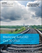
Sample lines are the engine underneath both sections and materials and are held in a collection called sample line groups. A sample line group is always associated with an alignment and can be found under the associated alignment in Prospector, as shown in Figure 13.1.

Figure 13.1 A view of Prospector; sample lines are held in a collection called a sample line group and are dependent on an alignment.

You can also see in Figure 13.1 that quite a few additional items are dependent on sample lines, such as sections, section views, mass haul lines, and mass haul views. If you click a sample line, you will see it has three types of grips, as shown in Figure 13.2.

Figure 13.2 The three grips on a sample line

To create a sample line group, change to the Home tab and choose Sample Lines from the Profile & Section Views panel. After selecting the appropriate alignment, the Create Sample Line Group dialog shown in Figure 13.3 will display. You should name the sample line group and verify the sample line and label style.

Figure 13.3 The Create Sample Line Group dialog

Every source object that is available will be displayed at the bottom of this box. If you wish to omit specific data from the section view, you can clear the check box. Set the applicable style for each item by clicking in the column to the right of the object. The section layer should be preset as specified in your template settings.

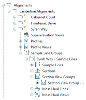
Once you've selected the sample data, the Sample Line Tools toolbar will appear, as shown in Figure 13.4.

Figure 13.4 From the Sample Line Tools toolbar, choose By Range Of Stations.

The By Range Of Stations option is used most often. You can use At A Station to create one sample line at a specific station. From Corridor Stations allows you to insert a sample line at each corridor assembly insertion. Pick Points On Screen allows you to pick any two points to define a sample line. This option can be useful in special situations, such as sampling a pipe on a skew. The last option, Select Existing Polylines, lets you define sample lines from existing polylines.

To define sample lines, you need to specify a few settings. Figure 13.5 shows these settings in the Create Sample Lines – By Station Range dialog. Right Swath Width is the width from the alignment that you sample. Most of the time this distance is greater than the ROW distance. You can also select Sampling Increments and choose whether to include special stations, such as horizontal geometry (PC, PT, and so on), vertical geometry (PVC, high point, low point, and so on), and superelevation critical stations.

Figure 13.5 Create Sample Lines – By Station Range dialog

In the following exercise, you'll create sample lines for Cabernet Court:

1. Open the SampleLines.dwg (SampleLines_METRIC.dwg) file, which you can download from this book's web page at www.sybex.com/go/masteringcivil3d2013.

2. Select the Home tab ⇒ Profile & Section Views panel and click Sample Lines.

3. At the Select an alignment, or press enter key to select from list>: prompt, press to display the Select Alignment dialog.

4. Select the Syrah Way alignment and click OK.

The Create Sample Line Group dialog opens.

5. In the Create Sample Line Group dialog:

a. Name the group Syrah Way-Sample Lines.

b. Clear the check boxes to the right of the PRELIM corridor and its surface named PRELIM Prelim.

c. Set surface EG to style Existing Ground by clicking in the Style column to the right.

d. Set the style for surface Intersection1 (Cab-Syrah) Corridor Top to Finished Ground.

The column is too narrow to view the full names of the items, so to see the name of the item pause your cursor over the name or expand the column.

e. Set the corridor Intersection1 (Cab-Syrah) style to All Codes.

6. When your dialog looks similar to Figure 13.3 (your sampled items may be listed in a different order), click OK.

7. On the Sample Line Tools toolbar, click the Sample Line Creation Methods drop-down arrow and then select By Range Of Stations.

8. In the Create Sample Lines – By Station Range dialog, leave the swath widths and sampling increments at their defaults (this will be 50′ for Imperial units and 20 m for metric units).

9. Change both the At Range Start and At Range End options to True, as shown earlier in Figure 13.5.

10. Click OK, and press to end the command.

11. If you receive a Panorama view telling you that your corridor is out of date and may require rebuilding, dismiss it by clicking the green check box.

You should now have dashed lines at even station intervals; these are your new sample lines.

12. Save the drawing for use in the next exercise.

Editing the Swath Width of a Sample Line Group

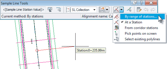
There may come a time when you need to show information outside the limits of your section views or not show as much information. To edit the width of a section view, you will have to change the swath width of a sample line group. These sample lines can be edited manually on an individual basis, or you can edit the entire group at once.

Sample Line and Section View Words of Wisdom

It is extremely rare to encounter situations where you need to touch each sample line or section view individually. Select a sample line or section view to access many time- (and sanity-) saving tools from the contextual tab.

You want to Change All the Sample Line Lengths

To change many swath widths at once:

1. Open the Sample Line Group Properties ⇒ Sample Lines tab, as shown here:

2. Select the first station you wish to change and hold down Shift as you click the last row.

3. Change the swath widths as desired.

You will need to change both the left and the right, because they are independent from each other.

You Want to Add or Remove Section Data in Many Views

A common situation with sections is that surface or corridor data you've created after you created sample lines is not appearing in your cross sections. This is easily rectified:

1. Click Sample More Sources.

Data that exists but that is not recognized by the sample lines will appear to the left, as shown here:

2. Highlight the data you wish to add, and click Add.

---

In this exercise, you'll edit the widths of an entire sample line group. You must complete the previous exercise before proceeding.

1. Continue working on the SampleLines.dwg (SampleLines_METRIC.dwg) file.

2. Select a sample line.

3. From the Sample Line contextual tab ⇒ Modify panel, click Group Properties.

4. Switch to the Sample Lines tab.

5. Click to select the first sample line in the listing at station 0+00.00 (0+000.00).

a. Scroll down to the bottom of the list.

b. While holding the Shift key, select the last station in the listing. This will highlight all rows.

c. Click your cursor in the Left Offset column and change it to 100′ (30 m).

d. Press to complete the edit.

After a moment, the left offsets should change.

e. With all of the rows still highlighted, make the same change to the Right Offset column.

6. Click OK.

After a moment the sample lines will resize to reflect your change.

7. Save the drawing.

Creating Section Views

Once the sample line group is created, it is time to create views. You can create a single view or many views arranged together (Figure 13.6).

Figure 13.6 Section views arranged to plot by page

A section view is nothing more than a window showing the section. The view contains horizontal and vertical grids, tick marks for axis annotation, the axis annotation itself, and a title. Views can also be configured to show horizontal geometry, such as the centerline of the section, edges of pavement, and right of way. Tables displaying quantities or volumes can also be shown for individual sections.

Creating a Single-Section View

There are occasions when all section views are not needed. In these situations, a single-section view can be created. In this exercise, you'll create a single-section view of station 0 + 00.00 (0+000.00) from sample lines:

1. Open the SectionViews.dwg (SectionViews _METRIC.dwg) file, which you can download from this book's web page.

You will want to switch to this drawing, since there are a few steps completed for you that you will learn later in the chapter.

2. Select the sample line at 0+50.00 (0+020.00).

3. From the Sample Line contextual tab ⇒ Launch Pad ⇒ Create Section view, select Create Section View.

4. Verify that your alignment, sample line group name, and station are correct on the General page of the wizard, as shown in Figure 13.7.

Figure 13.7 The General page of the Create Section View wizard

You can navigate from one page to another by either clicking Next at the bottom of the screen or clicking the links on the left side of the screen.

5. Click Next to view the Offset Range page.

The top of Figure 13.8 shows the Offset Range page, which should match your sample line swath width. In this case, as in the vast majority of cases, you will leave this set to Automatic. No action is needed on the Offset Range page.

Figure 13.8 The Offset Range page (top) and Elevation Range (bottom) of the Create Section View wizard

6. Click Next to view the Elevation Range page.

The bottom of Figure 13.8 shows the Elevation Range page. The values shown here are taken from your design max and min elevations. In this case, as in the vast majority of cases, you will leave this set to Automatic. No action is needed on the Elevation Range page.

7. Click Next to view the Section Display Option page.

The fourth page contains the section display options, as shown in Figure 13.9. This page reflects the styles and data you selected when creating your sample lines. If you forgot to set a style or wish to omit additional data, you can change your options here. No action is needed on the Section Display Options page.

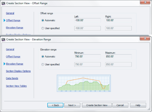
Figure 13.9 The Section Display Options page of the Create Section View wizard

8. Click Next to view the Data Bands page.

The fifth page, shown in Figure 13.10, lets you specify the data band options. Here, you can select band sets to add to the section view, pick the location of the band, and choose the surfaces to be referenced in the bands. No action is needed on the Data Bands page.

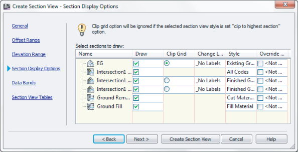
Figure 13.10 The Data Bands page of the Create Section View wizard

9. Click Next to view the Section View Tables page.

The sixth and last page, shown in Figure 13.11, is where you set up the section view tables. Note that this screen will be available only if you have already computed materials for the sample line group. On this page, you can select the type of table and the table style, and select the position of the table relative to the section view. Notice the graphic on the right side of the window that illustrates the current settings.

Figure 13.11 The Section View Tables page of the Create Section View wizard

10. With the table type set to Total Volume and the Select Table Style set to Basic, click Add.

As shown in Figure 13.11, you will have a line indicating that a material table will come in to the right of your view.

11. Click Create Section View.

12. Pick any point in the drawing area to place your section view.

13. Examine your section view.

The display should resemble Figure 13.12.

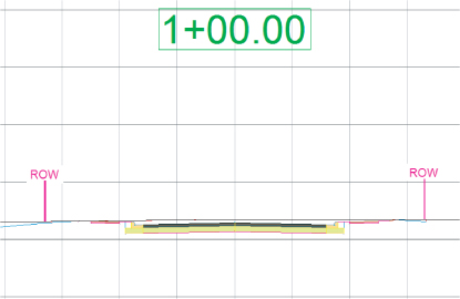
Figure 13.12 The finished section view

14. Save the drawing for use in the next exercise.

Creating Multiple Section Views

Section views belong in packs. In the exercise that follows, you will create section views intended to plot together on a sheet. (It is not necessary to have completed the previous exercise to continue.)

1. Continue working in SectionViews.dwg (SectionViews_METRIC.dwg).

2. Select any sample line.

3. From the Sample Line contextual tab ⇒ Modify Panel ⇒ Create Section view, select Create Multiple Section Views.

Alternately, you can access this tool from the Home tab ⇒ Profile & Section Views ⇒ Section Views ⇒ Create Multiple Views.

4. On the General page, set the Section View Style option to Road Section–No Grids, and click Next.

5. On the Section Placement page, click the ellipsis next to the path for Template For Cross Section Sheet.

6. From the default cross section sheet template, select ARCH D Section 20 Scale (ISO A1 Section 1 to 500), as shown in Figure 13.13, and click OK.

Figure 13.13 When you're creating multiple views, options allow for neat-looking groups.

7. Set Group Plot Style to Grid By Page, and click Next.

Figure 13.13 is a page you did not see when placing a single view. Setting the Production radio button allows you to use the Create Section Sheets tool from the Output tab. The Draft option forces Civil 3D to behave like version 2010 and prior.

Group Plot Style controls how the views are arranged on a page. In this example, the grid will come from the Group Plot style rather than the Section View style.

You can skip the rest of the wizard because you will keep the default input for the remainder of the settings.

8. Click Create Section Views.

9. Click anywhere off to the right of the graphic to place the views.

You should see views arranged on the screen (Figure 13.14). Metric users will see one page of section views, and Imperial unit users will see three pages of section views.

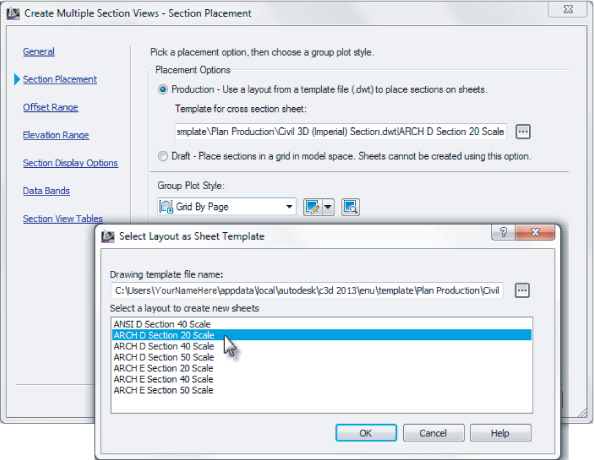
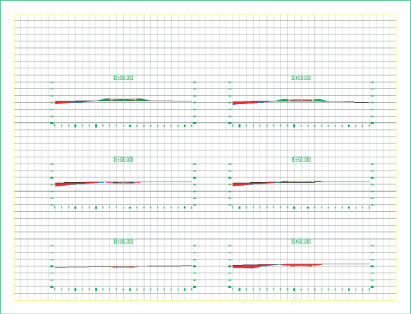
Figure 13.14 One of the pages of cross-section views

10. Save the drawing for use in the next exercise.

Delete Section Views the Pain-Free Way

The best way to remove an unwanted batch of section views from your graphic is to delete them through Prospector. In the following graphic you see the intrepid user tried (and apparently failed) seven times before keeping the view group.

If you delete views graphically, you'll create more work for yourself. First, the section view group stays behind in Prospector, as you see in the following image. As indicated by the dot in front of the group, only group 8 and the individual section view contain information.

The second problem with graphically deleting your section views is that Civil 3D interprets this maneuver as removing data from the sample lines. The next time you create sections, not all of the data you expect will be there. In this case, you would need to use the Sample More Sources tool to bring back the missing data.

The best way to delete section view groups is by right-clicking the group from Prospector and selecting Delete.

Section Views and Annotation Scale

In the previous exercise, you created section views using a cross-section sheet template. In step 6, you chose a scale. Coincidentally, the scale you used in the exercise was already set as the annotation scale. Since both scales agreed with each other, everything came out nicely.

Depending on what portion of the design you are working on, the scale of the sections and the scale you are comfortable working with may not agree. Additionally, you may just forget to set the scale ahead of placing section views.

Ideally, your section views and their sheets should be in a drawing separate from the corridor and the rest of the design. In Chapter 18, “Advanced Workflows,” you will learn how to do this using data shortcuts.

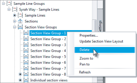
In the meantime, it is helpful to learn how to work with annotation scale and section views. In the following exercise, you will go through a brief lesson in reorganizing sections. You need to have completed the previous exercise before continuing.

---

Showing ROW Lines in Cross Section Views

The trick you are about to learn will come in handy for more than just showing right-of-way locations in cross section. Any item that is alignment-based can work the same way.

1. Open the drawing SectionROW.dwg (SectionROW_METRIC.dwg).

2. Select any sample line, and then from the Sample Line contextual tab ⇒ Modify panel, click Group Properties.

3. Switch to the Section Views tab.

4. Locate the Profile Grade column for the section view group. You may need to expand the columns to read what they are.

5. Click the ellipsis, as shown here:

The offset alignments represent the ROW location. An existing ground profile has been created for you as well. You will use this information to place the ROW symbol in the cross-section graphic.

6. Set Syrah Way Right 33.000 (Syrah Way Right 11.000) as the active alignment in the listing, and click Add.

7. Repeat step 6 for Syrah Way Left 33.000 (Syrah Way Left 11.000).

8. Set the Marker Style option for both left and right alignments to ROW Marker.

9. Click OK several times until you are out of all dialog boxes.

You should now have a ROW symbol whose insertion offset was determined by the alignment, and whose elevation was from the surface profile.

---

It's a Material World

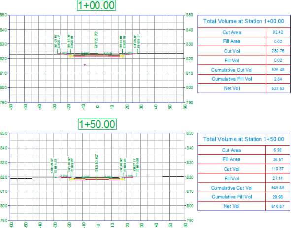
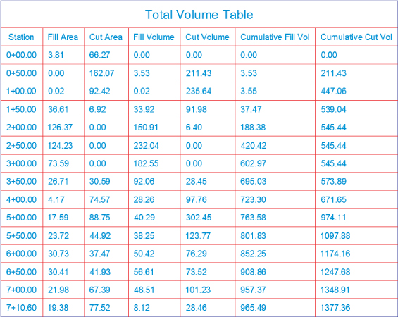
Once alignments are sampled, volumes can be calculated from the sampled surface or from the corridor section shape. These volumes are calculated in a materials list and can be displayed as a label on each section view or in an overall volume table, as shown in Figure 13.15.

Figure 13.15 A total volume table inserted into the drawing

The volumes can also be displayed in an XML report, as shown in Figure 13.16.

Figure 13.16 A total volume XML report shown in Microsoft Internet Explorer

Once a materials list is created, it can be edited to include more materials or to make modifications to the existing materials. For example, soil expansion (fluff or swell) and shrinkage factors can be entered to make the volumes more accurately match the true field conditions. This can make cost estimates more accurate, which can result in fewer surprises during the construction phase of any given project.

Creating a Materials List

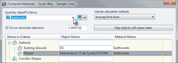
Materials can be created from surfaces or from corridor shapes. Surfaces are great for earthwork because you can add cut or fill factors to the materials, whereas corridor shapes are great for determining quantities of asphalt or concrete. In this exercise, you practice calculating earthwork quantities for the Syrah Way corridor:

1. Open the Materials.dwg (Materials _METRIC.dwg) file, which you can download from this book's web page.

2. Select the Analyze tab ⇒ Volumes And Materials panel and click Compute Materials.

The Select A Sample Line Group dialog appears.

3. In the Select Alignment field, verify that the alignment is set to Syrah Way, and then click OK.

The Compute Materials dialog appears.

4. In the Quantity Takeoff Criteria drop-down box, select Earthworks from the drop-down menu.

5. Click the Object Name cell for the Existing Ground surface, and select EG from the drop-down menu.

6. Click the Object Name cell for the Datum surface, and select Concord Commons Corridor Concord Commons Datum (this is the name of the corridor followed by the name of the surface) from the drop-down menu.

7. Verify that your settings match those shown in Figure 13.17, and then click OK.

Figure 13.17 The settings for the Compute Materials dialog

Graphically, nothing will happen. However, in the background Civil 3D has computed material data.

8. Save the drawing for use in the next exercise.

Creating a Volume Table in the Drawing

In the preceding exercise, materials were created that represent the total dirt to be moved or used in the sample line group. In the next exercise, you insert a table into the drawing so you can inspect the volumes. You need to have successfully completed the previous exercise before proceeding.

1. Continue working in Materials.dwg (Materials _METRIC.dwg).

2. Select the Analyze tab ⇒ Volumes And Materials and click Total Volume Table.

The Create Total Volume Table appears.

3. Verify that your settings match those shown in Figure 13.18.

Figure 13.18 The Create Total Volume Table dialog settings

4. Verify that Reactivity Mode at the bottom of the dialog is set to Dynamic.

This will cause the table to update if any changes are made to the corridor or related objects. Split Table should be enabled by default, so you can leave that as is.

5. Click OK.

6. Pick a point in the drawing to place the volume table.

The table indicates a Cumulative Fill Volume of 965.49 cubic yards (715.20 cubic meters) and a Cumulative Cut Volume of 1377.36 cubic yards (901.56 cubic meters), as shown previously in Figure 13.15.

7. Save the drawing for use in the next exercise.

Adding Soil Factors to a Materials List

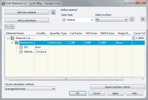
The material calculation indicates that this design has an excessive amount of fill. The materials need to be modified to bring them closer in line with true field numbers. For this exercise, the shrinkage factor will be assumed to be 0.80 and 1.20 for the expansion factor (20 percent shrink and swell). In addition to these numbers (which Civil 3D represents as Cut Factor for swell and Fill Factor for shrinkage), you can specify a Refill Factor value. This value specifies how much cut can be reused for fill. For this exercise, assume a Refill Factor value of 1.00. You need to have successfully completed the previous exercises before proceeding.

1. Continue working in Materials.dwg (Materials _METRIC.dwg).

2. Select the Analyze tab ⇒ Volumes And Materials panel and click Compute Materials.

The Select A Sample Line Group dialog appears.

3. Select the Cabernet Court alignment and the SL Collection–3 sample line group, if not already selected, and click OK.

The Edit Material List dialog appears.

4. Enter a Cut Factor of 1.20 and a Fill Factor of 0.80.

5. Verify that all other settings are the same as in Figure 13.19, and click OK.

Figure 13.19 The Edit Material List dialog

6. Examine the Total Volume table again.

Notice that the new Cumulative Fill Volume is 772.39 cubic yards (572.16 cubic meters) and the new Cumulative Cut Volume is 1652.84 cubic yards (1081.87 cubic meters).

7. Save the drawing.

Generating a Volume Report

Civil 3D provides you with a way to create a report that is suitable for printing or for transferring to a word processing or spreadsheet program. In this exercise, you'll create a volume report for the Concord Commons corridor. You need to have successfully completed the previous exercises before proceeding.

Section View Final Touches

Before you move away from section views, a few last touches are needed in your sections. First you will add last-minute data to the sections. You will also add labels to the sections.

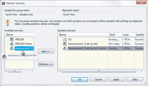
Sample More Sources

It is a fairly common occurrence that data is created from the design after sample lines have been generated. For example, you may need to add surface data or pipe network data to existing section views.

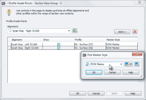
To accomplish this, you need to add that data to the sample line group. In this exercise, you'll add a pipe network to a sample line group and inspect the existing section views to ensure that the pipe network was added correctly:

1. Open the FinalTouches.dwg (FinalTouches_METRIC.dwg) file, which you can download from this book's web page.

2. Select one of the section views by clicking on the station label.

3. In the Section View contextual tab ⇒ Modify Section panel, click Sample More Sources.

4. Click Sanitary Network on the left side of the dialog to highlight it, as shown in Figure 13.20, and click Add.

Figure 13.20 Adding sewer data to the cross-section view via Sample More Sources

The Sanitary network will now appear on the right side of the dialog.

5. Click OK to dismiss the Section Sources dialog.

6. Save the drawing for use in the next exercise.

Cross-Section Labels

The best way to label cross sections that contain corridor data is using the code set style. Using the code set style you can control which parts of the corridor are labeled. You can learn more about creating code set styles in Chapter 20, “Label Styles.” In the meantime, you will look at how to change the code set style active on a cross-section view group.

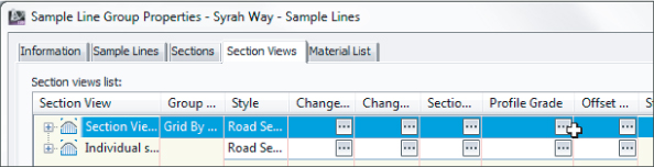
In the following exercise, you will use the view group properties to add labels. It is not necessary to have completed the previous exercise before continuing.

1. Continue working in the FinalTouches.dwg (FinalTouches_METRIC.dwg) file.

2. Select one of the section views by clicking on its station label.

3. In the Section View contextual tab ⇒ Modify View panel, click View Group Properties.

4. On the Sections tab, locate the Style column for the corridor and click the field that currently reads All Codes.

This is the code set style that is current in the views.

5. Switch the style to All Codes w Labels, as shown in Figure 13.21, and click OK.

Figure 13.21 Changing the active code set style for all views in the group

You should now have lovely little labels on all of the views, as shown in Figure 13.22.

Figure 13.22 Slope, elevation, and offset labels from the code set style

6. Save and close the drawing.

Mass Haul

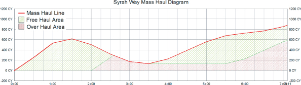
Mass haul diagrams help designers and contractors gauge how far and how much soil needs to be moved around a site. Figure 13.23 shows the mass haul diagram for Syrah Way. The Free Haul Area is material the contractor has agreed to move at no extra charge. The fact that the mass haul line is always above 0 indicates that the project is in a net cut situation through the length of the Syrah Way alignment.

Figure 13.23 Syrah Way Mass Haul diagram

Taking a Closer Look at the Mass Haul Diagram

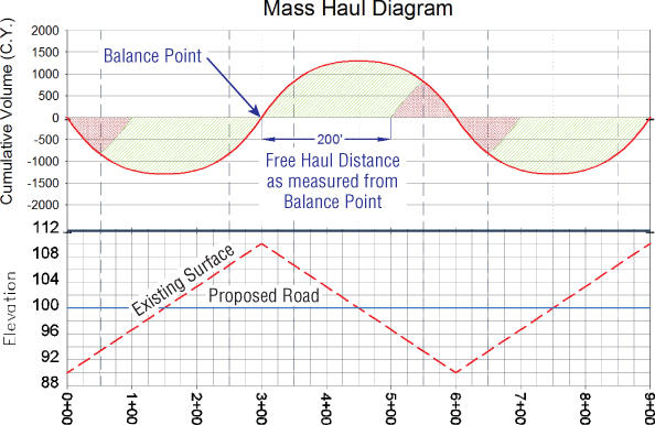
In an ideal design situation, there is no leftover cut material and no extra material needs to be brought in. This would mean that net volume = 0. When the line appears above the zero volume point, it is showing net cut values.

As the mass haul diagram continues, it shows the cumulative effect of net cut and fill for the alignment. When the net cut and net fill converge at the zero volume, the earthwork along the alignment is balanced. When the line appears below the zero volume point, it is showing net fill values, as you can see in Figure 13.24.

Figure 13.24 The volume, net cut, and net fill on an idealized mass haul diagram shown with profile

Here is some of the terminology you will encounter:

Create a Mass Haul Diagram

Now, let's put it all together and build a mass haul diagram in Civil 3D for Syrah Way and you'll see how easy it is:

1. Open the MassHaul.dwg (MassHaul_METRIC.dwg) file.

Remember, you can download all the data files from this book's web page.

2. From the Analyze tab ⇒ Volumes And Materials panel, select Mass Haul.

The Create Mass Haul Diagram dialog opens.

3. On the General page:

a. Verify that you are creating a mass haul diagram for Syrah Way alignment.

b. Verify that you are using the Syrah Way–Sample Lines group.

c. Leave all other options at their defaults, as shown in Figure 13.25, and click Next.

Figure 13.25 The Create Mass Haul Diagram dialog, General options

On the Mass Haul Display Options page, no changes are needed.

4. Click Next.

5. In the Balancing Options area, place a check box next to Free Haul Distance.

6. Set the distance to 200′ (60 m), as shown in Figure 13.26, and click Create Diagram.

Figure 13.26 The Create Mass Haul Diagram dialog, Balancing Options page

7. Find a clear spot on your drawing to place the mass haul diagram.

The diagram should look similar to Figure 13.23 (shown previously).

Editing a Mass Haul Diagram

When you create a mass haul diagram, you can easily modify parameters and get instant feedback on your diagram. Follow these steps to see how (you must have completed the previous exercise before continuing):

1. Continue working in the MassHaul.dwg (MassHaul_METRIC.dwg) file.

2. Select anywhere on the mass haul object or grid.

If you look at your mass haul diagram, you can see that nearly all the earthwork for Syrah Way involves net cut, which means hauling away dirt.

The Balancing options give you a chance to change or add waste and borrow pits. You will now make a few changes and observe what happens to the mass haul diagram.

3. From the Mass Haul View contextual tab ⇒ Modify panel, select Balancing Options.

The Mass Haul Line Properties dialog opens. It looks similar to part of the Balancing Options page shown earlier.

4. The Free Haul Distance is presently set for 200′ (60 m). Change it to 500′ (150 m).

5. Drag the dialog away from the screen to see the changes and then click Apply.

You can further tweak this amount to cut down on the net cut values by adding a dump site.

6. Click the Add Dump Site button.

a. Set the station to 1+31.00 (0+040.00).

b. Set the capacity to 850 cubic yards. (500 cubic meters).

7. When your dialog resembles the top of Figure 13.27, click OK.

Figure 13.27 The Mass Haul Line Properties dialog: adding a dump site (top). The mass haul diagram adjusted for the dump site (bottom)

The mass haul diagram will immediately update to reflect the changes, as shown at the bottom of Figure 13.27.

8. Save the drawing.

For this stretch of the project the mass haul diagram ends near zero. The changes you made also decrease the amount of overhaul in the project, decreasing potential cost.

The Bottom Line