Chapter 9
Custom Subassemblies
The stock subassemblies available with the AutoCAD® Civil 3D® software are capable of providing many solutions to your corridor needs, as discussed in Chapter 8, “Assemblies and Subassemblies.” However, there are going to be instances when what they offer isn't exactly what you need. Sometimes it may be too robust or sometimes not robust enough. When you install Civil 3D 2013, you are given the option to install an additional program called Autodesk® Subassembly Composer for AutoCAD® Civil 3D® (hereafter referred to as Subassembly Composer). This standalone program allows you to create custom subassemblies with an easy-to-use interface without having to know how to write programming code. These custom subassemblies can then be imported into Civil 3D for use in your assembly and corridor creation right alongside the stock subassemblies.
In this chapter, you will learn to:
- Define input and output parameters with default values
- Define target offsets, target elevations, and/or target surfaces
- Generate a flowchart of subassembly logic using the elements in the Tool Box
- Import a custom subassembly made with Subassembly Composer into Civil 3D
The User Interface
The Subassembly Composer is a separate program that is optionally installed when you install the Civil 3D software. Once you've installed it, select Start ⇒ All Programs ⇒ Autodesk ⇒ Subassembly Composer 2013 to launch the Autodesk Subassembly Composer 2013. The Subassembly Composer consists of five individual window panels: Tool Box, Flowchart, Properties, Preview, and Settings and Parameters (Figure 9.1).

Each of these window panels may be moved around independently by clicking on the panel's title bar and dragging it while using the docking control icons that appear to serve your needs. At any time you can return to the default position by choosing View ⇒ Restore Default Layout.
Tool Box
The Tool Box panel, which by default is located along the left side of the user interface, is the storage location for elements available for constructing the subassembly. This is similar to how the Tool Palettes panel in Civil 3D serves as the storage location for subassemblies available for constructing assemblies.
This panel will provide all the elements used to build your flowchart. There are five branches that can each be expanded and contracted to show the elements within that category: Geometry, Advanced Geometry, Auxiliary, Workflow, and Miscellaneous. To use any of these elements you click on the desired element and drag and drop it over into the Flowchart panel. You will look more closely at all the elements available later in this chapter.
Flowchart
The Flowchart panel, which by default is located at the top center of the user interface, is the workspace used to build and organize the subassembly logic and elements. A flowchart could be a simple straight line of logic, or it can be a complex tree of branching decisions. Either way, the subassembly definition always begins at the Start element. If there is a problem with your subassembly's logic, a small red circle with an exclamation point will be displayed in the upper-right corner of this panel.
Properties
The Properties panel, which by default is located at the bottom center of the user interface, is the input location of the parameters that define each geometry element. This is where you will spend most of your time defining the subassembly's geometry.
Preview
The Preview panel, which by default is located at the upper right of the user interface, allows you to view your subassembly as currently defined by the Flowchart panel. There are two preview modes:
Roadway Mode
Shows the subassembly built using any target surfaces, target elevations, and/or target offsets.
Layout Mode
Shows the subassembly built using only the input parameters (no targets).
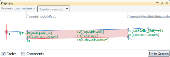
At the bottom of this panel are two check boxes: Codes and Comments. If any codes or comments were entered in the properties for the points, links, or shapes and you select these check boxes, this information will be listed next to the applicable geometry in the Preview pane. Codes will be shown in brackets [ ] and comments will be shown in parentheses ( ). You will learn how to define code and comments a little later. Use the rolling wheel on your mouse to zoom in and out or click the Fit To Screen button to zoom extents.
Settings and Parameters
The Settings and Parameters panel, which by default is located at the bottom right of the user interface, consists of five tabs that define the subassembly: Packet Settings, Input/Output Parameters, Target Parameters, Superelevation, and Event Viewer. You will take a closer look at each of these in this chapter.
Creating a Subassembly
Every subassembly that you create using the Subassembly Composer will be built using the same five basic steps:
1. Define the packet settings.
2. Define the input and output parameters.
3. (Optional) Define the target parameters.
4. Build the flowchart that defines the subassembly.
5. Save the packet (PKT) file in the Subassembly Composer and import it into Civil 3D.
The names in each of these steps should sound familiar, as many of them are built into specific sections of the user interface. Generally you will start in the Settings and Parameters panel in the lower-right corner of the user interface and work across the tabs from left to right to define the packet settings, input and output parameters, and then the target parameters. Then you will move over to the Tool Box, Flowchart, and Properties panels to define your subassembly. There are two other tabs in the Settings and Parameters panel: Superelevation and Event Viewer.
Defining the Subassembly
As you saw in Chapter 8, there are some instances when the stock subassemblies just aren't going to do what you need them to do to meet your design. One example of such a scenario (which you learned about in Chapter 8) was the inability to define different cross-slopes in the stock subassembly UrbanSidewalk for the inside boulevard (terrace), sidewalk, and the outside boulevard (buffer strip). To achieve the result you wanted, you used three separate subassemblies: a generic link, a sidewalk, and another generic link, which all worked independently of one another. Instead of always using this combination of subassemblies, you could generate a custom subassembly using Subassembly Composer in order to meet your specific design needs.
As you can see from the five basic steps discussed earlier, the first three are all about defining various components of your subassembly. These first three steps are the first three tabs of the Settings and Parameters panel. In the following example you will go through these three steps and define your subassembly.
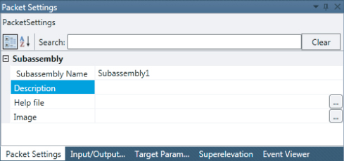
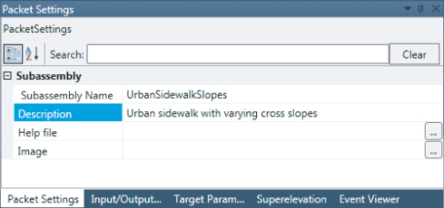
Packet Settings
On the Packet Settings tab shown in Figure 9.2, you can define the subassembly name, provide a description, link to a help file, and link to an image. Of these four pieces of information, only the subassembly name is required—the others are optional.
The subassembly name (which can be different from the name of the PKT file) will be the name that is displayed on the tool palettes once it's imported into Civil 3D. Like the stock subassemblies, the subassembly name that you define is not allowed to have any spaces.
If you include a description, this text will appear on the tool palette as hover text. Similarly, the image, if provided, will display in the tool palette next to the subassembly's name. We recommend that the image you provide be 224×224 pixels (although an image as small as 64×64 is allowed). If you create a help file, supply it in HTM or HTML format. To add an image or a help file, click the ellipsis button in that row and navigate to the file location.
Let's use this information to define the packet settings for this first example in a new subassembly PKT file. On the Packet Settings tab, do the following:
1. Set Subassembly Name to UrbanSidewalkSlopes or UrbanSidewalkSlopesMetric.
Remember, just like the stock subassemblies, your subassemblies can't have spaces in their names.
Metric or Imperial
Subassembly Composer is unitless. The same PKT file generated by the Subassembly Composer can be used in either the metric or the Imperial Civil 3D. The only difference is in default values: the Imperial subassembly will have all of these values based on feet and the metric subassembly will have all of these values based on meters. For this reason you are going to name your subassemblies differently so that you know which is which when they are later imported into the tool palettes in Civil 3D.
2. For Description, type Urban sidewalk with varying cross slopes.
You will notice that there are also Help File and Image options, which you will leave blank at this time since they are both optional.
The Packet Settings tab should now look like Figure 9.3.
Keep this file open to define the input and output parameters next.
Input and Output Parameters
On the Input/Output Parameters tab, shown in Figure 9.4, you can define numerous parameters along with their default values. These are the same as the input and output parameters that are available in the stock subassemblies (which you learned about in Chapter 8). The information on this tab is presented in a table. To add a parameter, simply click on the Create Parameter text. To remove a parameter, highlight that row in the table and press Delete on your keyboard.
Because this subassembly example is based on the UrbanSidewalk stock subassembly, it is good practice to keep terminology consistent with the stock subassembly for ease of use by the end user in Civil 3D.
Stock Subassemblies in Subassembly Composer
One of your first questions when running into a limitation with one of the stock subassemblies and wanting to make a modified subassembly based on the stock subassembly will likely be “Where can I find the PKT file for the stock subassemblies to use as a starting point?”
Unfortunately, at this time the stock subassemblies are written in a different type of code that does not allow them to be opened in Subassembly Composer. Let's hope that some of the stock subassemblies are made available in PKT format soon. In the meantime, creating a subassembly in Subassembly Composer based on one of the stock subassemblies is a great learning experience.
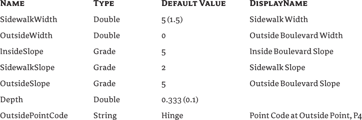
To stay consistent with the stock subassembly, let's look at the UrbanSidewalk help file for the input and output parameters that it uses. The help file indicates that there are six input parameters: Side, Inside Boulevard Width, Sidewalk Width, Outside Boulevard Width, %Slope, and Depth. You will use these six input parameters; however, the whole reason you are using Subassembly Composer for this example is to allow the end user to specify different slopes for each of the components. Therefore, in addition to %Slope (which you will instead name SidewalkSlope), you will define an Inside Boulevard Slope and an Outside Boulevard Slope. You will also give the end user the ability to specify a point code at the outside point numbered P4 in the help file.
The help file also indicates that there are no output parameters, so you will also not be defining any output parameters in this example.
As you look at the help file for the UrbanSidewalk subassembly, you may notice that the different input parameters have a type assigned to them. These same types are available in Subassembly Composer.
Input/Output Parameter Types
Eight input and output parameter types are provided with the program and accessible through the drop-down list in the Type column.
The eight variable types are:
- Integer, which is a whole number
- Double, which is a number that allows decimal precision
- String, which is text
- Grade, which is a percentage slope
- Slope, which is a ratio of horizontal distance to vertical distance
- Yes/No, which is used for Boolean variables
- Side, which can be set to Left, Right, or None
- Superelevation, which can be set to LeftInsideLane, LeftInsideShoulder, LeftOutsideLane, LeftOutsideShoulder, RightInsideLane, RightInsideShoulder, RightOutsideLane, RightOutsideShoulder, or None. The values of these cross slopes can be set on the Superelevation tab in the Settings/Parameters panel.
You can also create custom types, called enumerations, which will be discussed later in this chapter.
Let's use the help file information to define the input parameters for the example started in the previous exercise. On the Input/Output Parameters tab, do the following:
1. Change the default value for the Side input parameter to Right.
If you leave Default Value as None, this parameter will not be listed in the Advanced Parameters for the subassembly in Civil 3D. In a later symmetric example, you will leave this value set to None.
2. Click Create Parameter to add a new parameter.
3. Change Name to InsideWidth.
4. Verify that Type is set to Double by using the drop-down list.
5. Verify that Direction is set to Input by using the drop-down list.
6. Set Default Value to 0.
7. Set DisplayName to Inside Boulevard Width.
8. Click Create Parameter seven times to add seven more parameters. Alternatively you can click Create Parameter before defining each parameter.
Don't forget that if you add too many parameters, highlight that row in the table that you want to remove and press Delete on your keyboard.
Since you want all of these to be input parameters, all the Direction values will remain as Input.
9. Define the remaining seven input parameters with the following settings (note that the metric values are shown in parentheses if different from the Imperial values):
The program will change the parameters with the type of Grade to have a percent sign in the Default Value column. The DisplayName for Depth is intentionally left blank. The Description column is optional and any that are left blank will use Name as the DisplayName.
The Input/Output Parameters tab should now look like
Figure 9.5.
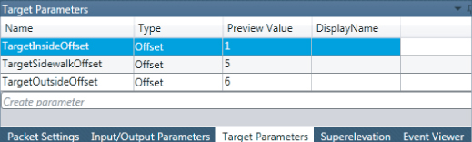
Target Parameters
On the Target Parameters tab, shown in Figure 9.6, you can define the targets to be used by the subassembly. You can use three types of targets:
- Offset targets
- Elevation targets
- Surface targets
These are the same types of targets that you learned about in Chapter 8.
As with the Input/Output Parameters tab, to add a parameter you click on the Create Parameter text, and to remove a parameter you highlight that row in the table and press Delete on your keyboard.
Just as you looked in the UrbanSidewalk help file for the input parameters that it uses, you will look in the help file for the target parameters. The help file indicates that there are three target parameters: Inside Boulevard Width, Sidewalk Width, and Outside Boulevard Width. The help file also indicates that these are optional. While the UrbanSidewalk file called all of these widths, they are actually offsets measured from the subassembly origin. Therefore, you are going to suffix the names of these targets with the word Offset.
Let's use this information to define the target parameters for this example. On the Target Parameters tab, do the following:
1. Click Create Parameter to add a new parameter, and then do the following:
a. Change Name to TargetInsideOffset.
b. Verify that Type is set to Offset.
c. Set Preview Value to 1 (or 0.25 for metric).
The preview value is different from the default value you defined for the input parameters. A preview value is used for graphical purposes and the actual value is generated based on the assigned targets.
2. Click Create Parameter to add a new parameter, and then do the following:
a. Change Name to TargetSidewalkOffset.
b. Verify that Type is set to Offset.
c. Set Preview Value to 5 (or 1.5 for metric).
3. Click Create Parameter to add a new parameter, and then do the following:
a. Change Name to TargetOutsideOffset.
b. Verify that Type is set to Offset.
c. Set Preview Value to 6 (or 1.75 for metric).
The Target Parameters tab should now look like
Figure 9.7.
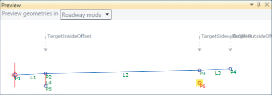
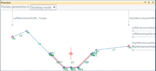
As you add the target parameters, you should notice that they will be added to the Preview panel, as shown in Figure 9.8, if you have the Preview Geometry option set to Roadway Mode. Remember, Roadway Mode will show your subassembly based on the target parameter, and Layout Mode will show your subassembly without the targets considered.
You can zoom in and out in your Preview panel by scrolling the mouse scroll wheel and pan by clicking the mouse scroll wheel and dragging. Once there are elements shown in the Preview panel, you can also zoom to the extents of your subassembly using the Fit To Screen button at the bottom-right corner of the panel, but the Fit To Screen button does not consider the target parameters.
Now that you have defined the subassembly parameters, you will start building the subassembly. You may keep this file open to continue on to the next exercise or use the finished copy of this file available from the book's web page, www.sybex.com/go/masteringcivil3d2013. The file is named UrbanSidewalkSlopes_Defined.pkt or UrbanSidewalkSlopesMetric_Defined.pkt.
Building the Subassembly Flowchart

Every flowchart will start from the appropriately named Start element. From there the flowchart is built with elements from the Tool Box, which are connected together with arrows. As you will see, every element that you add from the Tool Box has at least two nodes: one node for an incoming connection arrow and one node for an outgoing connection arrow.
Building a flowchart is as simple as dragging and dropping elements from the Tool Box into the Flowchart panel, as shown in this series of steps:
1. If it is still open from the previous exercise, continue working in the PKT file from the previous example or open the UrbanSidewalkSlopes_Defined.pkt or UrbanSidewalkSlopesMetric_Defined.pkt file.

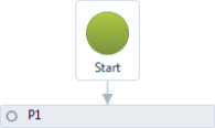
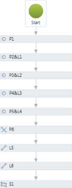
2. From the Tool Box ⇒ Geometry branch, drag a Point element to below the Start element.
The Start element will automatically connect to the new Point element, which has automatically been numbered P1, as shown in
Figure 9.9.
If you look at the Properties panel while point P1 is selected, you will see that it has been placed on the origin. The origin is the geometry point that your subassembly will attach to when generating an assembly in Civil 3D. While you may have instances where you don't want a point at the origin, it is generally the case that P1 and the origin will be coincident. As such, you do not need to change any of the defaults for this point.
P, AP, L, AL, and S Number Prefixes
While there are all sorts of geometric elements available in your Tool Box, they all boil down to three types: points, links, and shapes. These should all be familiar from the discussions in Chapter 8. Of the points and links there are regular points and links as well as auxiliary points and links. Auxiliary elements will be used for the purposes of calculations in Subassembly Composer but will never be displayed in Civil 3D.
In the Subassembly Composer, all points are prefixed with the letter P, all auxiliary points are prefixed with the letters AP, all links are prefixed with the letter L, all auxiliary links are prefixed with the letters AL, and all shapes are prefixed with the letter S. If you try to change this prefix for any of the elements you will get an error dialog.
Every element has to have a unique number. Subassembly Composer therefore will automatically number your elements with the next available appropriate number; if you want, you can change this number to one that is available but not to one that is already in use.
If you want to name your elements so that you can keep track of what they represent, instead of trying to put this information in the Number field, put it in the Comment field located at the bottom of the Properties panel.

3. From the Tool Box ⇒ Geometry branch, drag another Point element to below P1.
This point will be automatically numbered P2, and will represent the end of the Inside Boulevard and the start of the Sidewalk.
4. Define point P2 as follows:
a. Set Point Codes to “Sidewalk_In”.
Note that the quote marks are required in order to define this text as a string. If you are defining the point codes using a variable that is already defined as a string, the quotes are not needed.
b. Verify that Type is set to Slope And Delta X, as shown in
Figure 9.10.
c. Verify that From Point is set to P1.
d. Set Slope to InsideSlope.
e. Set Delta X to InsideWidth.
f. Set Offset Target (Overrides Delta X) to TargetInsideOffset.
Figure 9.11 shows the current Preview panel with the two point elements being generated. Notice that the element currently being displayed in the Properties panel (in this case point P2) is highlighted in yellow in the Preview panel. If your P2 appears to be in the same location as P1 in the Preview panel, zoom into P1 or click the Fit To Screen button.
g. Verify that the Add Link To From Point check box is selected. This link will automatically be numbered L1.
While you could add a link element from the Tool Box as a separate element after this point, this check box allows you to combine the two elements into one. This option is not available if the From Point is set to Origin or if the From Point is an auxiliary point when you are creating a point, or vice versa.
The P2 element in the Flowchart panel will change to now read P2&L1, as shown in
Figure 9.12. In addition, both P2 and L1 will be highlighted in the Preview panel.
h. Set the Link ⇒ Codes to “Top”, “Datum”.
While you only defined one code for the point, you want two codes for this link to be consistent with the UrbanSidewalk subassembly. You can add multiple codes by generating a comma-delimited list.
The properties for point P2 should now look like
Figure 9.13.

5. From the Tool Box ⇒ Geometry branch, drag another Point element to below P2&L1.
This point will be automatically numbered P3 (or P3&L2), and will represent the end of the Sidewalk and the start of the Outside Boulevard.
6. Define point P3 as follows:
a. Set Point Codes to “Sidewalk_Out”.
b. Verify that Type is set to Slope And Delta X.
c. Verify that From Point is set to P2.
d. Set Slope to SidewalkSlope.
e. Set Delta X to SidewalkWidth.
f. Set Offset Target (Overrides Delta X) to TargetSidewalkOffset.
g. Verify that the Add Link To From Point check box is selected.
This link will automatically be numbered L2.
h. Set Link ⇒ Codes to “Top”, “Sidewalk”.
Point P3 and link L2 are shown highlighted in
Figure 9.14.

7. From the Tool Box ⇒ Geometry branch, drag another Point element to below P3&L2.
This point will be automatically numbered P4, and will represent the end of the Sidewalk and the start of the Outside Boulevard.
8. Define point P4 as follows:
a. Set Point Codes to OutsidePointCode.
The UrbanSidewalk subassembly doesn't provide a code at point P4, but the ability to add codes wherever you want is another one of the benefits of using Subassembly Composer. Notice that unlike the previous point codes, you did not need to specify the quote marks on this one because this is a string variable that you created in the input/output parameters.
b. Verify that Type is set to Slope And Delta X.
c. Verify that From Point is set to P3.
d. Set Slope to OutsideSlope.
e. Set Delta X to OutsideWidth.
f. Set Offset Target (Overrides Delta X) to TargetOutsideOffset.
g. Verify that the Add Link To From Point check box is selected.
This link will automatically be numbered L3.
h. Set the Link ⇒ Codes to “Top”, “Datum”.
Point P4 and link L3 are shown highlighted in
Figure 9.15.

9. From the Tool Box ⇒ Geometry branch, drag another Point element to below point P4 and link L3.
This point will be automatically numbered P5, and will represent the bottom of the sidewalk shape directly below point P2.
10. Define point P5 as follows:
a. Verify that Type is set to Delta X And Delta Y.
b. Verify that From Point is set to P2.
Because you are basing point P5 on point P2, wherever point P2 is located P5 will always remain in relation to it. So point P5 will follow the target offset already defined for point P2.
c. Set Delta X to 0.
d. Set Delta Y to –Depth.
e. Verify that the Add Link To From Point check box is selected.
This link will automatically be numbered L4.
f. Set the Link ⇒ Codes to “Sidewalk”, “Datum”.
Point P5 and link L4 are shown highlighted in
Figure 9.16.
The last point to define is point P6 at the inside bottom of the sidewalk shape directly under point P3. You could define point P6 in the same way you just defined point P5, as a –Depth from point P3, but in order to show a variety of element types, you will instead define it using an intersection point. An intersection point is classified the same as a regular point, so it will have the same P prefix as all the other points you already defined.
Intersection Point Geometry Types
There are three intersection point geometry types. These types are applicable to both intersection points and auxiliary intersection points. These types are as follows:
Intersection: LinkPointSlope
To define an intersection by LinkPointSlope, you will need to have a link and a point with a slope from the point. The new point will be placed at the intersection of the link and the projected slope.
In addition there are three Geometry Properties check boxes: Extend Link, Extend Slope, and Reverse Slope. The Extend Link and Extend Slope check boxes convert the link or slope from a segment (link) or ray (point with slope) into a line that extends beyond its original extents in order to find the desired intersection if no direct intersection is available. The Reverse Slope check box reverses the slope (i.e., a slope of 25% is treated as –25%).
Intersection: TwoLinks
To define an intersection by TwoLinks, you will need to have two links. The new point will be placed at the intersection of these two links.
In addition there are two Geometry Properties check boxes: Extend Link 1 and Extend Link 2. These have the same type of behavior as the extending check boxes previously discussed.
Intersection: TwoPointsSlope
To define an intersection by TwoPointsSlope, you will need to have two points and a slope from each of these points. The new point will be placed at the intersection of these two projected slopes.
In addition there are four Geometry Properties check boxes: Extend Slope 1, Extend Slope 2, Reverse Slope 1, and Reverse Slope 2. These have the same type of behavior as the extending and reversing check boxes previously discussed.
With all of the intersection types, if an intersection is not found, no point is generated.

11. From the Tool Box ⇒ Advanced Geometry branch, drag an Intersection Point element to below point P5 and link L4.
This point will be automatically numbered P6, and will represent the outside bottom of the sidewalk shape directly below point P3.
12. Define intersection point P6 as follows:
a. Verify that Type is set to Intersection: TwoPointsSlope.
b. Verify that Point 1 is set to P5.
c. Set Slope 1 to SidewalkSlope.
This assumes that the slope of the sidewalk does not change. If this subassembly had an elevation target that could override the cross-slope of the Top link (L1), you would instead want to set this variable to L1.slope. This annotation is called an application programming interface (API) function. You will learn about many other API functions later in this chapter.
d. Verify that Point 2 is set to P3.
e. Set Slope 2 to -Infinity%.
You could alternatively set Slope 2 to Infinity% and select the Extend Slope 2 check box.

13. From the Tool Box ⇒ Geometry branch, drag a Link element to below P6.
This link will be automatically numbered L5, and will represent the datum of the sidewalk shape.
14. Define link L5 as follows:
a. Set Link Codes to “Sidewalk”, “Datum”.
b. Verify that Start Point is set to P5.
c. Verify that End Point is set to P6.

15. From the Tool Box ⇒ Geometry branch, drag another Link element to below L5.
This link will be automatically numbered L6, and will define the vertical outside edge of the sidewalk shape, thus closing the shape. When adding a shape element, you must have a closed set of links.
16. Define link L6 as follows:
a. Set Link Codes to “Sidewalk”, “Datum”.
b. Verify that Start Point is set to P6.
c. Verify that End Point is set to P3.
Link L5 and link L6 are shown highlighted in
Figure 9.18.

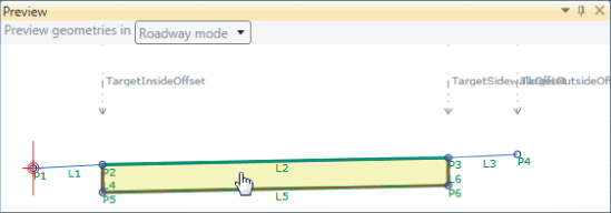
17. From the Tool Box ⇒ Geometry branch, drag a Shape element to below L6.
This shape will be automatically numbered S1 and will define the sidewalk shape.
18. Define link S1 as follows:
a. Set Shape Codes to “Sidewalk”.

b. Click the Select Shape In Preview button.
To pick the shape, do not take time to figure out the name of each link and try to use Add Link and type in the links. Instead, by clicking the green Select Shape In Preview button to the right of the entry field, you can then click inside the shape in the Preview panel, just like you would when defining a hatch in AutoCAD. If you are working with a subassembly that has multiple closed shapes and want to change to a different shape, click the green selection icon again and reselect the new shape—there's no need to delete the previously listed links; the list of links will update for you.
c. Select inside the closed shape representing the sidewalk, as shown in
Figure 9.19.
Once you generate all of your points, links, and shapes, it is good practice to select the Codes check box in the bottom-left corner of the Preview panel to confirm that all the desired codes have been assigned, as shown in Figure 9.20. You want to check to make sure that the links have the desired link codes, that the points have the desired point codes, and that the shapes have the desired shape codes.
You can keep this file open to continue on to the next exercise or use the finished copy of this file available from the book's web page. The file is called UrbanSidewalkSlopes_Flowchart.pkt or UrbanSidewalkSlopesMetric_Flowchart.pkt.
Keeping the Flowchart Organized
As you built the subassembly in the previous exercise, you should have noticed all the connection arrows that were automatically created between the elements. If you click and drag any of the elements around, the connection arrows will bend and twist to maintain the connection. Therefore, if you want to reorder your elements you will need to delete the connection arrows, reposition the elements, and redraw the connection arrows.
If you highlight one of the connection arrows and press Delete on your keyboard, the connection will break. As you are building and troubleshooting your subassemblies, you may find it useful to occasionally delete a connection arrow so that you can confirm that everything above an element is in working order. To redo a broken connection, click on the starting element to display the connection nodes and click and drag from one of the connection nodes to the desired node on the next element.
You may notice that with even a simple subassembly such as the previous example, the Flowchart panel starts to fill up quickly. You can enlarge the Flowchart work area by clicking and dragging on the lower-right corner. In addition to the default Flowchart work area, you can nest workflow inside your flowchart, like you nest folders on your computer to organize information.
In general there are two types of flowchart workflows:
Sequence Workflow
This is a straight sequential series of elements.
Flowchart Workflow
This can be a straight series of elements or a branching complex series of decisions and elements.
Both of these workflows can be found in the Workflow branch of the Tool Box. In the previous example, you placed each element one after another into the flowchart, as shown in Figure 9.21.
When you have a sequence of elements like this, it is often cleaner to put them into a Sequence element. In our next exercise, you will move the subassembly elements into a sequence:
1. If it is still open from the previous exercise, continue working in the PKT file from the previous example, or open the UrbanSidewalkSlopes_Flowchart.pkt or UrbanSidewalkSlopesMetric_Flowchart.pkt file.
2. Delete the first connection arrow from the Start to point P1.

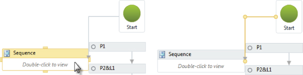
3. From the Tool Box ⇒ Workflow branch, drag a Sequence element to an open area near the Start element.
Notice that because it is off to the side, the connection arrow connected to the side of the Sequence element instead of the top like in the previous exercise. There are actually four or more nodes on each of the elements that connection arrows can connect to. You can see these connection nodes when you hover over an element.
4. To change the connection node of the connection arrow, click on the connection arrow to display the grips shown in
Figure 9.22.
5. Click on the grip at the arrow end of the connection arrow and drag it to the desired connection node at the top of the Sequence element.
You can do the same thing with the opposite end of the connection arrow to connect out of the bottom of the Start element if desired.
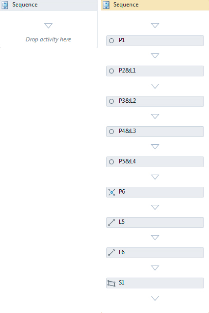
6. Click on one of the elements in your flowchart.
7. Press and hold the Ctrl key on your keyboard and continue to click on each of the elements in your flowchart.
8. Press Ctrl+X to cut the elements from the flowchart.
If you want to duplicate some of the elements in your flowchart instead of move them, you can use Ctrl+C and Ctrl+V. The duplicated points, links, and shapes will be renumbered with the next available numbers.
9. Double-click on the Sequence element to enter the sequence.
The sequence will be empty, as shown at the left in
Figure 9.23.
10. Press Ctrl+V to paste the elements into the sequence, as shown at the right in
Figure 9.23.
Now you can easily shuffle the elements around if desired.
11. To return to the Flowchart area, click on the word
Flowchart in the upper-left corner of the Flowchart panel, as shown in
Figure 9.24.
Compare Figure 9.25 to Figure 9.21 shown earlier, and you will see how much room a Sequence element can save.
In addition, you can click on the word Sequence on the element to rename the element. This can be helpful if you want to combine and organize groups of common elements, such as a sequence for each layer of pavement in a multiple-layer subassembly.
When this exercise is complete, you can close the file. A finished copy of this file is available from the book's web page with the filename UrbanSidewalkSlopes_Sequence.pkt or UrbanSidewalkSlopesMetric_Sequence.pkt.
Importing the Subassembly into Civil 3D
To import your subassembly into the Civil 3D tool palettes, use the following steps:
1. If you haven't already done so, in Subassembly Composer save your PKT file from the previous exercise and close the program.
2. Open Civil 3D and create a new drawing using the _AutoCAD Civil 3D (Imperial) NCS or the _AutoCAD Civil 3D (Metric) NCS template.
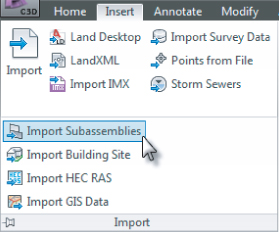
3. From the Insert tab ⇒ expanded Import panel, choose Import Subassemblies, as shown in
Figure 9.26.

The Tool Palettes window will open, if it's not already open, and the Import Subassemblies dialog will be displayed.
4. In the Import Subassemblies dialog, click the folder button to display the Open dialog.
5. Navigate to your saved UrbanSidewalkSlopes.pkt or UrbanSidewalkSlopesMetric.pkt file and click Open.
6. Verify that the Import To: Tool Palette check box is selected.
7. Using the drop-down list, select Create New Palette from the bottom of the list to display the New Tool Palette dialog.
Custom Tool Palette for Custom Subassemblies
By creating a new tool palette you can keep all of your custom subassemblies in one easy-to-find location. As you continue to make more subassemblies and test them, you may also find it helpful to have a tool palette named Testing in addition to your tool palette of confirmed working subassemblies.
8. For Name enter Mastering and click OK to return to the Import Subassemblies dialog.
The Import Subassemblies dialog should now look like
Figure 9.27.
9. Click OK to accept the settings in the Import Subassemblies dialog.
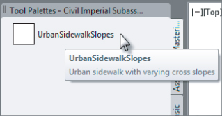
A new palette named Mastering will be added and it will contain your UrbanSidewalkSlopes subassembly. Since you did not specify an image, an empty white square is shown. But if you hover over the subassembly name, a tooltip will be displayed showing the description that you provided in Subassembly Composer, as shown in
Figure 9.28.
You can see how helpful the description can be if you provide your PKT file to a different user. You can now use this subassembly just as you would any other subassembly using the procedures discussed in Chapter 8, “Assemblies and Subassemblies.”
Using Expressions
In the UrbanSidewalkSlopes example, all of the dimensions and slopes were provided through the input parameters. There are going to be some instances when you want to perform more detailed calculations for the expressions in your various elements. For these instances you will turn to API functions to generate your expressions. The link API function L1.slope was briefly mentioned earlier but there are many more API functions that you have at your fingertips. These API functions are defined by classes. Each API function has at least two parts: one before the period and one after the period. Some API functions also call for additional information provided in parentheses. While you will find you use some API functions more than others, each has an important use. Let's summarize the API functions available in Subassembly Composer.
Point and Auxiliary Point Class API Functions
There are multiple API functions that you can call to provide information about points and auxiliary points. To use these API functions, you type the point you want information about and then a period, followed by the API function. For example, in order to get the horizontal distance from the origin to point P1, you would enter P1.X. The API functions in the Point class are as follows (shown for point P1; however, this can apply to any of the points or auxiliary points previously defined in the flowchart):
X
P1.X returns the horizontal distance from point P1 to the origin. A positive value means that point P1 is to the right of the origin, and a negative value means that point P1 is to the left of the origin.
Y
P1.Y returns the vertical distance from point P1 to the origin. A positive value means that point P1 is above the origin, and a negative value means that point P1 is below the origin.
Offset
P1.Offset returns the horizontal distance from the assembly baseline to point P1. A positive value means that point P1 is to the right of the assembly baseline, and a negative value means that point P1 is to the left of the assembly baseline.
Elevation
P1.Elevation returns the elevation of point P1 relative to elevation 0.
DistanceTo
P1.DistanceTo(“P2”) returns the distance from point P1 to point P2. This value is always positive. The quote marks are required unless you are defining the second point using another API function, such as the L1.StartPoint API function discussed later.
SlopeTo
P1.SlopeTo(“P2”) returns the slope from point P1 to point P2. If the value is positive it is an upward slope, or if it is negative it is a downward slope. The quote marks are required unless you are defining the second point using another API function such as the L1.StartPoint API function discussed later.
IsValid
P1.IsValid returns a value of True or False if the point P1 is assigned and valid.
DistanceToSurface
P1.DistanceToSurface(SurfaceTarget) returns the vertical distance from the point P1 to the target surface. A positive value means that point P1 is to the above the target surface, and a negative value means that point P1 is below the target surface.
Link and Auxiliary Link Class API Functions
Like points and auxiliary points, there are multiple API functions that you can call to provide information about links and auxiliary links. To use these API functions, you type the link you want information about and then a period, followed by the API function. For example, in order to get the slope of link L1, you would enter L1.Slope. The API functions in the Link class are as follows (shown for link L1; however, this can apply to any of the links or auxiliary links previously defined in the flowchart):
Slope
L1.Slope returns the slope of link L1.
Length
L1.Length returns the length of link L1. This value is always positive.
XLength
L1.XLength returns the horizontal distance between the start and end of link L1. This value is always positive.
YLength
L1.YLength returns the vertical distance between the start and end of link L1. This value is always positive.
StartPoint
L1.StartPoint returns a point located at the start of link L1. This can then be used in the API functions for the Point class.
EndPoint
L1.EndPoint returns a point located at the end of link L1. This can then be used in the API functions for the Point class.
MaxY
L1.MaxY returns the maximum Y elevation from a link's points.
MinY
L1.MinY returns the minimum Y elevation from a link's points.
MaxInterceptY
L1.MaxInterceptY(slope) returns the highest intercept of a given link's points to the start of another link.
MinInterceptY
L1.MinInterceptY(slope) returns the lowest intercept of a given link's points to the start of another link.
LinearRegressionSlope
L1.LinearRegressionSlope returns the slope calculated as a linear regression on the point in a link to find the best fit slope between all of them.
LinearRegressionInterceptY
L1.LinearRegressionInterceptY returns the Y intercept of the linear regression link.
IsValid
L1.IsValid returns a value of True or False if the link is assigned and valid to use.
HasIntersection
L1.HasIntersection(“L2”,true,true) returns a value of True or False if links L1 and L2 have an intersection. The second and third expressions are optional. If not defined, they both default to false. The second expression defines whether to extend link L1, and the third expression defines whether to extend link L2.
Elevation Target Class API Functions
There are multiple API functions that you can call to provide information about elevation targets. The API functions in the Elevation Target class are as follows (shown for an elevation target name ElevationTarget; however, this can apply to any of the elevation targets):
IsValid
ElevationTarget.IsValid returns a value of True or False if the elevation target is assigned and valid to use.
Elevation
ElevationTarget.Elevation returns the elevation of the elevation target relative to elevation 0.
Offset Target Class API Functions
There are multiple API functions that you can call to provide information about offset targets. The API functions in the Offset Target class are as follows (shown for an offset target name OffsetTarget; however, this can apply to any of the offset targets):
IsValid
OffsetTarget.IsValid returns a value of True or False if the offset target is assigned and valid to use.
Offset
OffsetTarget.Offset returns the horizontal distance from the assembly baseline to the offset target. A positive value means that the offset target is to the right of the assembly baseline, and a negative value means that the offset target is to the left of the assembly baseline.
Surface Target Class API Functions
There is one API function that you can call to provide information about surface targets. The API function in the Surface Target class is IsValid. It is shown here for a surface target name SurfaceTarget; however, this can apply to any of the surface targets:
SurfaceTarget.IsValid
This returns a value of True or False if the surface target is assigned and valid to use.
Baseline Class API Functions
There are multiple API functions that you can call to provide information about the assembly baseline. Unlike some of the other API functions that use the name of a specific element before the period, with the Baseline class API functions, all of them begin with the word Baseline. The API functions in the Baseline class are as follows:
Station
Baseline.Station returns the station of the assembly baseline at the current frequency line.
Elevation
Baseline.Elevation returns the elevation of the assembly alignment at the current frequency line.
RegionStart
Baseline.RegionStart returns the station at the start of the current corridor region.
RegionEnd
Baseline.RegionEnd returns the station at the end of the current corridor region.
Grade
Baseline.Grade returns the instantaneous grade of the assembly baseline at the current frequency line.
TurnDirection
Baseline.TurnDirection returns the turn direction of the current station on the baseline alignment.
Enumeration Type Class API Functions
There is one API function that you can call to provide information about a user-defined enumeration. The API function in the Enumeration Type class is Value. It is shown here for the enumeration name EnumerationType; however, this can apply to any of the enumerations:
EnumerationType.Value
This returns the string value of the current enumeration item.

Enumeration?
When you learned about the eight different types for input and output parameters earlier, the term enumeration was mentioned. Enumeration allows you to generate a unique type. The enumeration will generate a drop-down list of options in the Advanced Parameters properties category for the subassembly in Civil 3D, similar to the Yes/No drop-down list.
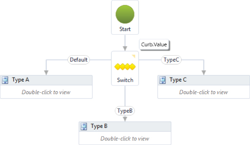
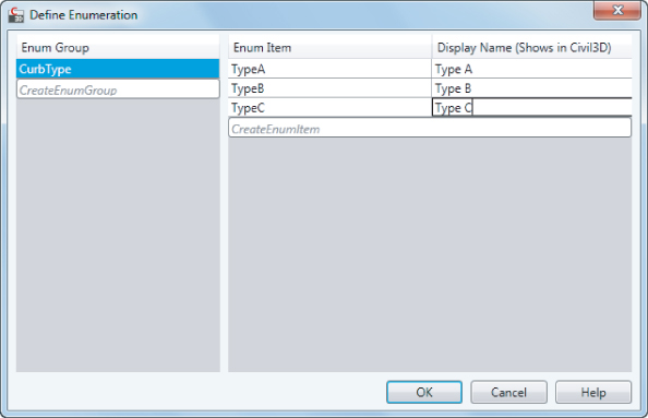
For example, if you had three different types of curbs, you could place a Switch element below the Start element and then build a sequence for each of the types of curbs and connect them to the Switch element as shown here:
If you create an enumeration group listing the three curb types (enumeration items), the end user can specify which curb they want from the subassembly's properties without having to change the dimensions to match the desired curb shape.
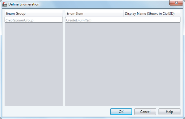
To create a custom enumeration, follow these steps:
1. From the View menu, select Define Enumeration to display the Define Enumeration dialog shown here:
2. Click CreateEnumGroup to add an enumeration group.
3. Change the enumeration group name from Enum0 to CurbType.
4. Click CreateEnumItem three times to add three items within the group.
5. Change the enumeration items to match the following image:
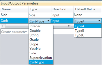
Now you can generate an input parameter with the type as CurbType and specify the default value from the enumeration items:
If you look back at the flowchart of the Switch element, you will notice a few things.
First, you will notice the Curb.Value enumeration class API function floating to the upper right of the Switch element. This flyout is available on both the Switch elements as well as the Decision elements; it shows the expression that is being used by the element. In this case, the expression calls for the value of the Curb input parameter.
Second, you will notice the three connection arrows coming out of the Switch element. Decision elements are used for deciding between two options (true or false), whereas Switch elements can actually handle 11 conditions. The first condition is always Default. The next conditions will default to Case1, Case2, and so on. You will want to change these to correspond with the other cases. You can change the case names by clicking on the connection arrow and changing the Case setting in the Properties panel.
Math API Functions
In addition to all the Subassembly Composer API functions, numerous math API functions are available. A few of the common ones you may find a need for are as follows:
Round
Math.Round(12.1009,2) returns the first value rounded to the nearest specified decimal places. If the second value is -2, it will round to the nearest hundreds, -1 will round to the nearest tens, 0 to the nearest integer, 1 to the nearest tenths, 2 to the nearest hundredths, and so on.
Floor or Ceiling
Math.Floor(12.1009) or Math.Ceiling(12.1009) returns the next smallest integer (floor) or next largest integer (ceiling). In this example, the floor would be 12 and the ceiling would be 13.
Max or Min
Math.Max(12.1009,4.038) or Math.Min(12.1009,4.038) returns the maximum value or minimum value of the two specified values. In this example, the max would be 12.1009 and the min would be 4.038.
Pi
Math.pi returns the value of the constant pi.
Sin, Cos, Tan, Asin, Acos, or Atan
Math.Sin(math.pi) returns sine of the specified value (in this case the constant pi). This similar format could be used for any of the other trigonometric functions. The angles specified or calculated should be provided in radians.
Using an API Function in an Expression
With all of the stock subassemblies, the parameters are constants throughout the region unless a target is used to taper the offset or elevation. By using the API functions in the baseline class, you can now generate a subassembly that knows the start and end of the region that it is in as well as the current station. By using this information, you can taper from a start value to an end value. In the following example, you will use the Subassembly Composer to calculate the current value (a double variable) based on the starting value and end value, which have a linear taper between them. You will then import this simple calculation subassembly into Civil 3D to use in tapering a shoulder using a parameter reference.
1. Start a new subassembly file and save it as TaperDouble.pkt.
2. On the Packet Settings tab, enter TaperDouble for the subassembly name.
3. On the Input/Output Parameters tab, click Create Parameter to add a new parameter for each of the input and output parameters with the following settings:
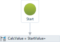
4. From the Tool Box ⇒ Geometry branch, drag a Point element to below the Start element.
Leave this point as generated at the origin and do not change any of the default values. A minimum of one point must be in the subassembly in order for the calculation that you will define in the next step to work once imported into Civil 3D.

5. From the Tool Box ⇒ Miscellaneous branch, drag a Set Output Parameter element to below P1.
6. Define the Set Output Parameter element as follows:
a. Verify that Output Parameter is set to CalcValue.
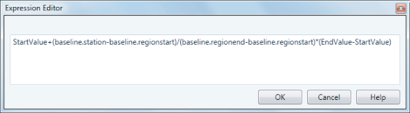
b. Set the value to StartValue+(baseline.station-baseline.regionstart)/(baseline.regionend-baseline.regionstart)*(EndValue-StartValue).
If you ever want to have a larger text field for entering text, many of the fields throughout the Subassembly Composer have an ellipsis button that you can click to display the Expression Editor dialog, as shown in
Figure 9.29.
7. In Subassembly Composer, save your PKT file, which should now look like
Figure 9.30.
When this portion of the exercise is complete, you can close the file. A finished copy of this file is available from the book's web page with the filename TaperDouble.pkt. You will now import this subassembly into Civil 3D and use a parameter reference to pass the output parameter into another subassembly as an input parameter.
8. Open the TaperShoulder.dwg or TaperShoulder_METRIC.dwg file.
This file has an assembly of a simple road cross section with lanes, curbs, shoulders, and daylight links, as shown in
Figure 9.31.
9. From the Insert tab ⇒ expanded Import panel, choose Import Subassemblies.
The Tool Palettes window will open, if it's not already open, and the Import Subassemblies dialog will be displayed.
10. In the Import Subassemblies dialog, click the folder button to display the Open dialog.
11. Navigate to your saved TaperDouble.pkt file and click Open.
12. Verify that the Import To: Tool Palette check box is selected and select the Mastering tool palette you created in an earlier exercise.
13. Click OK to accept the settings in the Import Subassemblies dialog and add the subassembly to the Mastering tool palette.
Now you will add the TaperDouble calculation before the left and right shoulders. The TaperDouble subassembly component will calculate the shoulder width and pass it to the shoulder subassembly using a parameter reference.
14. Click the TaperDouble subassembly on the Tool Palettes window.
15. Locate the Advanced-Parameters section on the Design tab of the AutoCAD Properties palette.
16. Change the Start Value to 3¢ (or 1 m) and the End Value to 10¢ (or 3 m).
17. At the
Select marker point within assembly or [Insert Replace Detached]: prompt, press
I 
.
18. At the
Select the subassembly to insert after or [Before]: prompt, press
B .
19. At the Select the subassembly to insert ahead of: prompt, select the left shoulder, which is a LinkWidthAndSlope subassembly.
20. At the
Select a different marker point on the new subassembly, or enter to continue: prompt, press
.
Now you will do the same thing to add the TaperDouble calculation before the right shoulder.
21. At the
Select the subassembly to insert after or [Before]: prompt, press
B .
22. At the Select the subassembly to insert ahead of: prompt, select the right shoulder.
23. At the
Select a different marker point on the new subassembly, or enter to continue: prompt, press
.
24. Press
again to end the command.
25. Right-click on the red assembly baseline marker and select Assembly Properties.
26. On the Construction tab, highlight the LinkWidthAndSlope subassembly in the Right group.
27. In the Input Values area, select the check box in the Parameter Reference Use column for the Width value.
28. In the Get Value From column next to the check box, select TaperDouble.Calculated Value, as shown in
Figure 9.32.
29. Repeat steps 26 through 28 for the Left group.
30. Click OK when complete.
Where Are the Shoulders and Daylight Links?
You will notice that the shoulders and daylight links appear to have disappeared from the assembly. This is because the shoulder links are trying to calculate based on their location in a region of a corridor and don't yet have anything to calculate. Don't worry—the subassembly elements are still there, as shown in the Assembly Properties that you just looked at. Just because the assembly does not look right doesn't mean that it is broken!
When this exercise is complete, you can close the drawing. A finished copy of this drawing is available from the book's web page with the filename TaperShoulder.dwg or TaperShoulder_Metric.dwg.
By passing the value to a stock subassembly, you avoid having to re-create the entire stock subassembly just to incorporate an API function into the calculation of one parameter.
Employing Conditional Logic
Decisions are the most common way you will define conditions that will have either a true or a false result. There are two ways you can make decisions: one is with a Decision or Switch element, and the other is by using conditional logic operators in your expression. If the decision is going to affect only one expression, then you will want to use the conditional logic operators. However, if the decision is going to have an effect on the flowchart logic, then you will use a Decision or Switch element.
Conditional Logic Operators
There are numerous conditional logic operators that you will want to be familiar with as you define decision conditions. Examples of these are as follows:
> or <
P1.Y>P2.Y (or P1.Y<P2.Y) returns true if P1.Y is greater than (or less than) P2.Y.
>= or <=
P1.Y>=P2.Y (or P1.Y<=P2.Y) returns true if P1.Y is greater than or equal to (or less than or equal to) P2.Y.
= or <>
P1.Y=P2.Y (or P1.Y<>P2.Y) returns true if P1.Y is equal to (or not equal to) P2.Y.
AND
P1.Y>P2.Y)AND(P2.X>P3.X) returns true if both the first condition located in a pair of parentheses and the second condition located in a pair of parentheses are true.
OR
(P1.Y>P2.Y)OR(P2.X>P3.X) returns true as long as at least one of the conditions located in either pair of parentheses is true.
XOR
(P1.Y>P2.Y)XOR(P2.X>P3.X) returns true if one of the conditions located in a pair of parentheses is true and the other condition located in a pair of parentheses is false.
Any of these operators could also be used in an If statement within any expression in order to test a condition and provide one of two different values.
In the following example expression for a slope value, the distance from auxiliary point AP1 to the target surface is calculated. If it is greater than 0, meaning that AP1 is located above the surface (in fill), then the slope value will be –0.25. If the value is not greater than 0, meaning that AP1 is located below the surface (in cut), then the slope value will be 0.33.
IF(AP1.DistanceToSurface(TargetSurface)>0,-0.25,0.33)
With a combination of the right conditional logic operators, you can make all kinds of decisions.
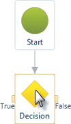
Decision and Switch Elements
You briefly saw an example of a Switch element in action earlier in this chapter when you learned about enumeration. The Decision elements have a similar behavior but provide only two conditions: True or False. The Decision element is located in the Tool Box ⇒ Workflow branch along with the Switch element, Flowchart element, and Sequence element. When you insert a Decision element into your flowchart and hover over it, you will see that the True condition will be out of the left side and the False condition will be out of the right side, as shown in Figure 9.33.
An easy way to remember which side is which is “Right side means the condition is wRong.”
By highlighting the element you can define the condition in the Properties panel. For example, you can specify AP1.DistanceToSurface(TargetSurface)>0 similar to the example expression discussed in the previous section. However, notice that you did not need to specify in the expression what will happen if the answer is true or false; this is because you will specify the true and false through the use of the connection arrows out of the left and right sides of the Decision element.
One of the benefits of using a Decision element in your flowchart instead of burying a conditional expression into an element is that finding them is easy, since the flowchart is a visual representation of the logic. There are a few things you can do to make your decisions easy to follow in the flowchart, as shown in Figure 9.34.
The first thing you can do is click on the triangular flag in the upper-right corner of the element. Doing this will cause the condition expression to be displayed in a flyout.
The second thing you can do is to further annotate the True and False connection arrow labels. You can change these labels through the Decision element's Properties panel.
You will also notice in Figure 9.34 that there are two elements named P1. This may confuse you, as you have learned up until this point that every point, link, and shape must have a unique number, which is true—however, there is a caveat. The elements must have a unique number along any given connection arrow path. Because these elements are not along the same path, they may be duplicated.
Making Sense of Someone Else's Thoughts
There is going to come a time that you will open a PKT file that someone else made or you made long ago. Most likely you are opening up this confusing and complicated PKT file because you have found a mistake in how it behaves in Civil 3D or you want to edit it for different Civil 3D capabilities. So instead of building the subassembly from scratch you will have to understand how the subassembly was built.
In this last example, you will open a complex subassembly that was made to behave similarly to the Channel stock subassembly. You have decided that instead of the baseline attachment point being at a point located above the midpoint of the bottom width, at a height equal to the Depth parameter, you want it at the midpoint of the bottom link.
1. Open the Channel.pkt or Channel_METRIC.pkt file.
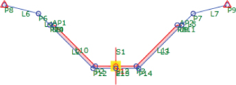
The channel subassembly in the Preview panel, as shown in
Figure 9.35, should look similar to the subassembly shown in the Channel stock subassembly help file.
As you can see, the flowchart is full of decisions and sequences and elements. Thankfully, if you take a close look you will see that the sequences are clearly labeled, as are the True and False labels, as shown in
Figure 9.37.
Because the attachment point is typically one of the first elements defined, it should be pretty easy to find.
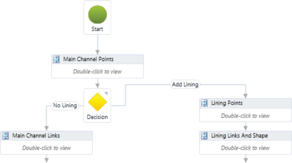
2. Double-click on the Main Channel Points sequence element.
Be certain to double-click on the actual element and not the text; otherwise you will just select the name of the sequence for editing.
3. Click on the element for point P1.
You will notice that it also highlights in the Preview panel.
4. In the Properties panel, change the Delta Y from -math.abs(Depth), as shown in
Figure 9.38, to
0.
When you do so, you will notice that the whole subassembly jumps up to the origin. You will also notice that the links at right have disappeared in Roadway Mode. This is because Roadway Mode uses the targets that are set at locations which are no longer valid. If you look at Event Viewer in the Settings/Parameters panel you will notice three errors about points that can be placed. These errors will disappear if you choose to change the preview values of the right target parameters. If you switch to Layout Mode, your subassembly will use only the input parameter that matches
Figure 9.39.
math.abs(Depth)?
You may have noticed the original expression that was used to define the Delta Y value of this point and wondered what it was doing. math.abs() is an API function that finds the absolute value of the variable in the parentheses. By first finding the absolute value of the input parameter, you avoid having an error occur if one user in Civil 3D thinks the Depth parameter should be a negative value and one user thinks it should be a positive value.
Although this was a simple change to a complex flowchart, it all starts with finding the right location to change the variable. Now that the attachment point is at the bottom of the channel, let's make one more change to this subassembly. You should add a link representing the water surface elevation and then define a shape for the water, as shown in the next steps.
5. In the Preview panel, zoom in to the subassembly and you will notice that the depth points located at the top of the lining of the channel are at point P4 on the left and point P5 on the right.
6. On the Input/Output Parameters tab, change the value for LiningDepth to 0.
You will notice that the lining disappears but the depth points remain as P4 and P5. This is good because it means that you can define one link as the water surface that will be applicable to the subassembly with and without the lining.
7. From the Tool Box ⇒ Geometry branch, drag a Link element to below point P5 in the Main Channel Points sequence.
This link will automatically be numbered L13.
8. Define link L13 as follows:
a. Set Link Codes to “WaterSurface”.
Note that the quote marks are required in order to define this text as a string.
b. Verify that Start Point is P4 and End Point is P5.
9. Click on the word Flowchart in the upper-left corner of the Flowchart panel to return to the main flowchart.
You must now find an appropriate place to define the shape delineating the water.
10. On the No Lining side of the first decision, double-click the Main Channel Links sequence element.
11. From the Tool Box ⇒ Geometry branch, drag a Shape element to below link L3. This shape will automatically be numbered S2.
12. Define shape S2 as follows:
a. Set Shape Codes to “Water”.
Note that the quote marks are required in order to define this text as a string.
b. Click the Select Shape In Preview button.
c. Select inside of the closed shape representing the water, as shown in
Figure 9.40.
13. On the Input/Output Parameters tab, change LiningDepth back to 0.333 (or 0.1 for metric).
Notice that the water link remains but the shape is no longer present. This is because you defined the shape in a branch of the flowchart that isn't being used when the lining is in place.
14. Click on the word Flowchart in the upper-left corner of the Flowchart panel to return to the main flowchart.
You must now find an appropriate place to define the shape delineating the water for the subassembly when a lining is being used.
15. On the Add Lining side of the first decision, double-click the Lining Links And Shape sequence element.
16. From the Tool Box ⇒ Geometry branch, drag a Shape element to below shape S1.
This shape will automatically be numbered S3. Note that if you wanted you could renumber this shape to S2 since it is located in a different branch from the S2 previously defined.
17. Define shape S3 as follows:
a. Set Shape Codes to “Water”.
Note that the quote marks are required in order to define this text as a string.
b. Click the Select Shape In Preview button.
c. Select inside of the closed shape representing the water, as shown in
Figure 9.41.
You have now changed the attachment point from the depth location to the bottom of the channel, added a link at the water elevation, and defined a water shape.
When this exercise is complete, you can close the file. A finished copy of this file is available from the book's web page with the filename Channel_modified.pkt or Channel_Metric_modified.pkt.
Sharing Custom Subassemblies
PKT files are not part of the drawing file. So anytime you use a PKT file in a drawing you must make the PKT file available for anyone who has to rebuild the corridor. If a user does not first import the subassembly into the drawing, they will receive an error message that says “One or more subassembly macros (or .NET classes) could not be found. Check Event Viewer for more information. Continue? Yes/No.”
In conjunction with the stock subassemblies already available in the Civil 3D and the custom subassemblies you create with the Tool Box in the Subassembly Composer, your corridors will have endless possibilities.
The Bottom Line
Define input and output parameters with default values.
By providing detailed input parameters, you let the Civil 3D user edit your custom subassembly. In addition, by providing detailed output parameters you let them use the subassembly's characteristics to edit the subsequent subassemblies in the assembly.
Master It
Generate a new subassembly PKT file for a subassembly named MasteringLane (or MasteringLaneMetric). For input parameters, define the following:
- Side with a default value of Right
- LaneWidth provided as a decimal precise number with a default value of 12 feet or 3.6 meters
- LaneSlope provided as a percentage with a default value of -3%
- Depth provided as a decimal precise number with a default value of 0.67 feet or 0.2 meters
For output parameters, define the following:
- CalcLaneWidth provided as a decimal precise number
- CalcLaneSlope provided as a percentage
Define target offsets, target elevations, and/or target surfaces.
Targets allow the subassembly to reference unique items within the drawing. They allow for varying widths, tapered elevations, and daylighting to a surface.
Master It
For the same subassembly from the previous Master It, define an elevation target named TargetLaneElevation with a preview value of -0.33 feet (or -0.1 meters) and an offset target named TargetLaneOffset with a preview value of 14 feet (or 4 meters).
Generate a flowchart of subassembly logic using the elements in the Tool Box.
The Tool Box in Subassembly Composer is full of all sorts of tools. But like a tool box in your garage, the tools are only useful if you know their capabilities and practice using them. The simplest tools are points, links, and shapes, but there are also tools for more complex flow charts.
Master It
Define the subassembly using the width, slope, and depth input parameters defined earlier. Make certain that if the slope of the lane changes based on the targets, then the top and the datum links have matching slopes.
The subassembly should have four points: P1 (“Crown”) located at the origin, P2 (“ETW”) located at the upper-right corner of the lane cross section (with both the TargetLaneElevation and TargetLaneOffset), P3 (“Crown_Subbase”) at the lower left of the lane cross section, and P4 (“ETW_Subbase”) at the lower right of the lane cross section.
The subassembly should have four links: L1 (“Top”, “Pave”) connecting P1 and P2, L2 connecting P1 and P3, L3 (“Datum”, “Subbase”) connecting P3 and P4, and L4 connecting P2 and P4.
The subassembly should have a shape: S1 (“Pave1”).
Import a custom subassembly made with Subassembly Composer into Civil 3D.
A custom subassembly is no good if it is just made and not used. By knowing how to import your PKT file into Civil 3D, you open up the world of building and sharing tool palettes full of subassemblies to help your office's workflow.
Master It
Import your MasteringLane or MasteringLaneMetric subassembly into Civil 3D.