Chapter 4
Surfaces
One of the most primitive elements in a three-dimensional model of any design is the surface. As you learned in the previous chapter, once survey information is gathered and points are set with elevations, you can proceed to turn some of that information into an intelligent surface. This chapter examines various methods of surface creation and editing. Then it moves into discussing ways to view, analyze, and label surfaces, and explores how they interact with other parts of your project.
In this chapter, you will learn to:
- Create a preliminary surface using freely available data
- Modify and update a TIN surface
- Prepare a slope analysis
- Label surface contours and spot elevations
- Import a point cloud into a drawing and create a surface model
Understanding Surface Basics
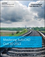
A surface in the AutoCAD® Civil 3D® program is generated using the principle of geometric triangulation. At the very simplest, a surface consists of points. In planar geometry, two points can be used to define a line and three points can be used to define a plane. Using this principle, the computer generates a triangular plane using a group of three points (Figure 4.1). Each of these triangular planes shares an edge with another, and a continuous surface is made. This methodology is typically referred to as a triangulated irregular network (TIN), as shown in Figure 4.2. On the basis of Delaunay triangulation, this means that for any given (x,y) point, there can be only one unique z value within the surface (since slope is equal to rise over run, when the run is equal to 0 the result is “undefined”). What does this mean to you? It means standard surfaces have two major limitations:
No Thickness
Modeled surfaces can be thought of as a sheet draped over a surface; they have no thickness in the vertical direction associated with them.
No Vertical Faces
Vertical faces cannot exist in a TIN because two points on the surface cannot have the same (x,y) coordinate pair. At a theoretical level, this limits the ability to handle true vertical surfaces, such as walls or curb structures. You must take this factor into consideration when modeling corridors, as discussed in Chapter 10, “Basic Corridors.”
Figure 4.1 Three points defining a plane

Figure 4.2 A triangulated irregular network, or TIN
Beyond these basic limitations, surfaces are flexible and can describe any object's face in astonishing detail. The surfaces can range in size from a few square feet to square miles and generally process quickly.
There are three main categories of surfaces in Civil 3D: standard surfaces, volume surfaces, and corridor surfaces. A standard surface is based on a single set of points, whereas a volume surface builds a surface by measuring vertical distances between two standard surfaces. Each of these two categories of surfaces can also be a grid or TIN surface. The grid version is still a TIN upon calculation of planar faces, but the data points are arranged in a regularly spaced grid of information. The TIN version is made from randomly located points that may or may not follow any pattern to their location. A corridor surface is generated from a corridor and will be discussed further in Chapter 10.
Creating Surfaces
![]()
Before you can analyze a surface, you have to make one. To the land development company today, this can mean pulling information from a large number of sources, including Internet sources, old drawings, and fieldwork. Working with each requires some level of knowledge about the reliability of the information and how to handle it in the Civil 3D software. In this section, we'll look at how you can obtain data from a couple of free sources and bring it into your drawing, create new surfaces, and make a volume surface.
Before creating surfaces, you need to know a bit about the components that can be used as part of a surface definition:
LandXML Files
These typically come from an outside source or are exported from another project. LandXML has become a common means of communicating data in the land development industry. These files include information about points and triangulation, making replication of the original surface as easy as a few mouse clicks.
DEM Files
Digital Elevation Model (DEM) files are the standard format files from governmental agencies and GIS systems. These files are typically very large in scale but can be great for planning purposes.
TIN Files
Typically, a TIN file comes from a land development project on which you or a peer has worked. These files contain the baseline TIN information from the original surface and can be used to replicate it easily.
Boundaries
Boundaries are closed polylines that determine the visibility of the TIN inside the polyline. The polyline can be a 2D polyline, a 3D polyline, or even a feature line, but only the horizontal information will be used to generate the boundary — any elevation information will not be used. Outer boundaries are often used to eliminate stray triangulation, whereas hide boundaries are used to indicate areas that could perhaps not be surveyed, such as a building pad. Note that only the area within a boundary is utilized in calculations. If the polyline that created the boundary is modified, the surface will become out of date, thus requiring a rebuild unless the surface is set to rebuild automatically.
Breaklines
Breaklines are used for creating hard-coded triangulation paths, even when those paths violate the Delaunay algorithms for normal TIN creation. They can describe anything from the top of a ridge to the flowline of a curb section. A TIN line may not cross the path of a breakline. A breakline cannot be added to a grid surface. Breaklines can be defined using 2D polylines, 3D polylines, or feature lines. Similar to boundaries, if a breakline is modified the surface will become out of date, thus requiring a rebuild. Breaklines will be discussed in more detail later in this chapter.
Contours
Sometimes a specific contour is desired, and it can be inserted into the surface as a 2D polyline at an elevation. Points will be placed along the contour to be used in the triangulation process. This process will be discussed in more detail later in this chapter. Similar to a breakline, a contour cannot be added to a grid surface. Similar to boundaries, if a breakline is modified, the surface will become out of date, thus requiring a rebuild. Adding contour data will be discussed further later in this chapter.
Drawing Objects
AutoCAD objects that have an insertion point at an elevation (e.g., text, blocks, lines, polylines, arcs, 3D polylines) can be used to populate a surface with points. It's important to remember that no relationship to the drawing object is maintained; only the point data associated with the drawing object is added to the surface, not the actual drawing object.
Edits
Any manipulation after the surface is completed, such as adding or removing triangles or changing the datum, will be part of the edit history. These changes can be viewed in the surface properties, where individual edits can be toggled on and off individually to make reviewing changes simple, or reordered since edits are implemented in the order that they are added.
Point Files
Point files work well when you're working with large data sets where the points themselves don't necessarily contain extra information. Examples include laser scanning or aerial surveys. A drawing will stay referenced to a point file. If the point file is moved or deleted, the reference in the drawing will be broken.
Point Groups
Civil 3D point groups or survey point groups can be used to build a surface from their respective members and maintain the link between the membership in the point group and being part of the surface. In other words, if a point is removed from a group used in the creation of a surface, it is also removed from the surface.
Working with all these elements, you can model and render almost any surface you'd find in the world. In the next section, you'll start building some surfaces.

Free Surface Information
You can find almost anything on the Internet, including information about your project site. Some of this information may be valuable in generating a surface to use for conceptual design. For most users, free surface information can be gathered from government entities as discussed in the following section.
Surfaces from Government Digital Elevation Models
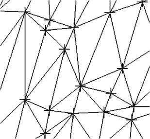
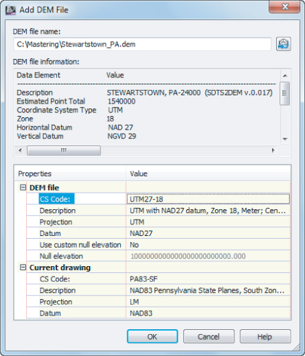
One of the most common forms of free data is the Digital Elevation Model (DEM). These files have been used by the U.S. Department of the Interior's United States Geological Survey (USGS) for years and are commonly produced by government organizations for their GIS systems. The DEM format can be read directly by Civil 3D, but the USGS typically distributes the data in a complex format called Spatial Data Transfer Standard (SDTS). The files can be converted using a freely available program named sdts2dem. This DOS-based program converts the files from the SDTS format to the DEM format you need. Once you are in possession of a DEM file, creating a surface from it is relatively simple, as you'll see in this exercise:
Figure 4.3 Imperial coordinate settings for DEM import
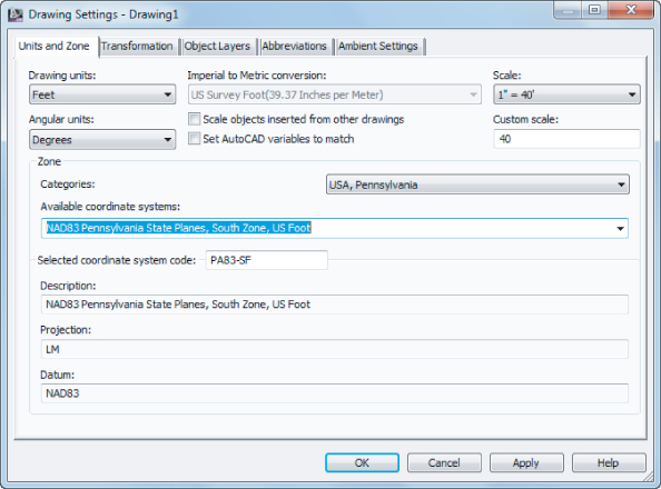
Figure 4.4 Adding DEM data to a surface

![]()
Figure 4.5 Setting the Stewartstown_PA.DEM coordinate zone
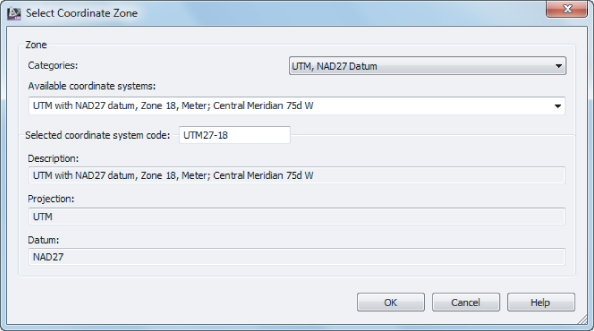
Figure 4.6 Setting the Stewartstown_PA.DEM file properties
Once you have the DEM data imported, you can pause over any portion of the surface and see that feedback showing the surface elevation is provided through a tooltip. This surface can be used for preliminary planning purposes but isn't accurate enough for construction purposes.
The main drawback to DEM data is the sheer bulk of the surface size and point count. The Stewartstown_PA.DEM file you just imported contains 1.4 million points and covers more than 55 square miles. This much data can be overwhelming, and it covers an area much larger than the typical site. If you try zooming in and out on the surface, you will notice that the computer will be slow as it tries to regenerate the surface with each change. To ease the processing and activate the Level Of Detail display, do the following:
![]()
After these steps are complete you will notice a new icon appears in the upper-left corner of your model space, showing you that Level Of Detail is activated. To turn off Level Of Detail, follow the same steps.
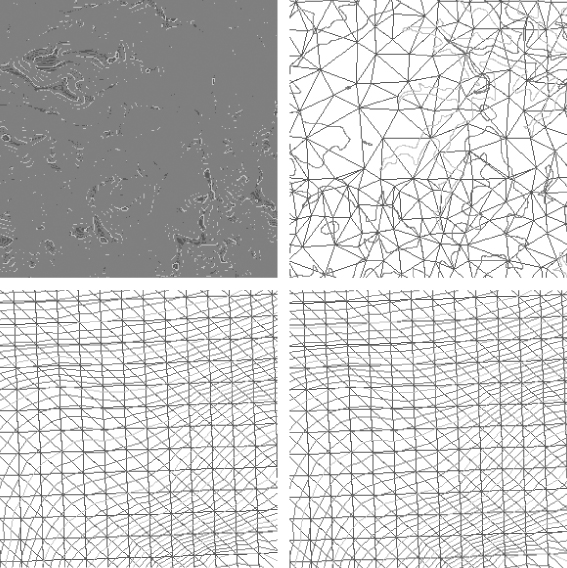
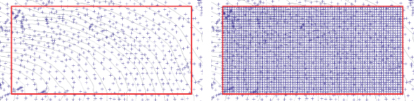
Turning on the Level Of Detail display does not change the data in the surface but simply changes what is viewable at the different zoom levels. Figure 4.7 shows the same area of the surface zoomed out and zoomed in before (left) turning on Level Of Detail and after (right). You'll look at some data reduction methods later in this chapter.
Figure 4.7 DEM surface: zoomed out without Level Of Detail (upper left), zoomed out with Level Of Detail (upper right), zoomed in without Level Of Detail (lower left), zoomed in with Level Of Detail (lower right)
In addition to making a DEM a part of a TIN surface, you can build a surface directly from the DEM:
The drawback to this approach is that no coordinate transformation is possible. Because one of the real benefits of using georectified data is pulling in information from differing coordinate systems, we're skipping this method to focus on the more flexible method shown in this exercise. When this exercise is complete, you may close the drawing. Due to the large file size, a finished state of this drawing is not available for download on the book's web page.
Surface from GIS Data
You may run into a situation where an outside firm uses GIS, or perhaps your firm is also using GIS data. Civil 3D understands GIS and can work with the data given. In this section, we'll show you how to import GIS data pertaining to surfaces:
Figure 4.8 The Create Surface From GIS Data – Object Options page
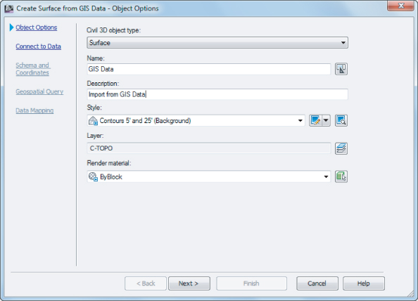
Figure 4.9 The Create Surface From GIS Data – Connect To Data page

Figure 4.10 The Create Surface From GIS Data – Schema And Coordinates page
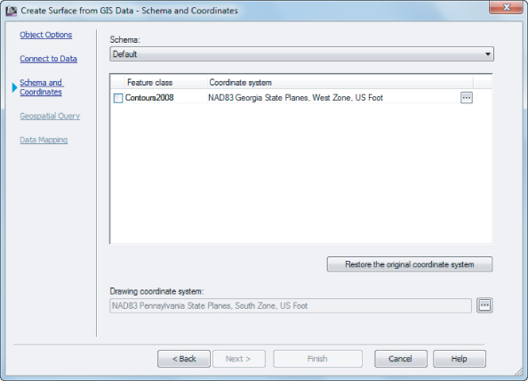
Figure 4.11 The Create Surface From GIS Data – Geospatial Query page

Figure 4.12 The Create Surface From GIS Data – Data Mapping page
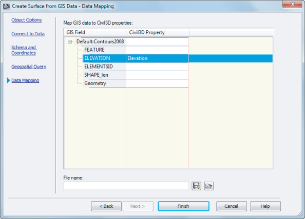
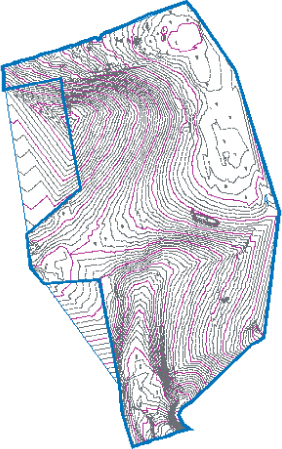
Figure 4.13 The finished imported GIS contours

This is just another avenue for getting drawings from other sources into Civil 3D. This topic will be discussed in depth in Chapter 18, “Advanced Workflows.”
Surface Approximations
In this section, you'll work with elevated polylines. Later in this chapter, you'll work with a large point cloud delivered as a text file. These polylines are quite common, and historically it can be difficult making an acceptable surface from them.
Surfaces from Polyline Information
One common complaint about converting a drawing full of contours at elevation into a working digital surface is that the resulting contours don't accurately reflect the original data. This is because point information is provided along the contour lines but not in between the contour lines, causing the interpolation between the contours to lack accuracy. Civil 3D includes a series of surface algorithms that work very well at matching the resulting surface to the original contour data by providing additional derived data points. You'll look at those surface edits in this series of exercises.
Figure 4.14 The Add Contour Data dialog
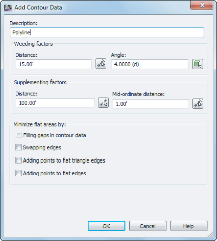
Figure 4.15 Contour surface without minimizing flat areas
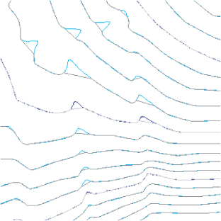
Figure 4.16 Contour surface with minimizing flat areas
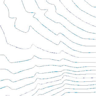
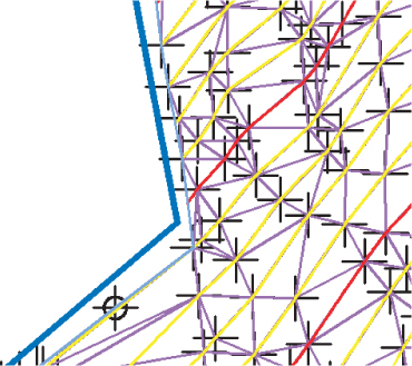
Figure 4.17 Surface data points and derived data points
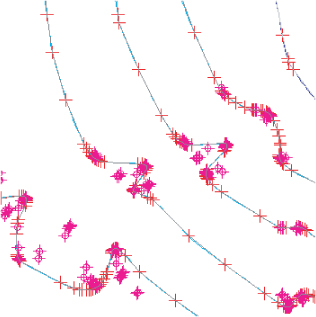
In Figure 4.17, you're seeing the points the TIN is derived from, with some styling applied to help you understand the creation source of the points. Each point shown as a red + symbol is a point picked up from the contour data itself. The magenta points shown with a circle symbol circumscribed over a + symbol are all added data on the basis of the Minimize Flat Areas edits. These points make it possible for the Civil 3D surface to match almost exactly the input contour data.
When this exercise is complete, you may close the drawing. A saved finished copy of this drawing is available from the book's web page with the filename SurfaceFromPolylines_FINISHED.dwg or SurfaceFromPolylines_METRIC_FINISHED.dwg.
Surfaces from Points or Text Files
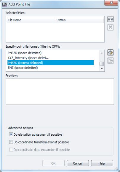
Besides receiving polylines, it is common for a surveying company to also send a simple text file with points. This isn't an ideal situation because you have no information about breaklines or other surface features, but it is better than nothing or usually more accurate than a surface based on free data. Because you have the same aerial surface described as a series of points, you'll use them to generate a surface in this exercise:
Figure 4.18 Adding a point file to the surface definition
![]()
Remove Snapshot
This option will remove the snapshot from the build operation.
Rebuild Snapshot
Rebuilding the snapshot and rebuilding the surface are in fact two different things. If the operations prior to the snapshot become outdated, you will see a yellow status icon next to its node in the Prospector tree prompting for the snapshot to be rebuilt. You can then choose to rebuild the snapshot if you want the changes to affect the surface or leave the snapshot in place as is if you do not want the changes to affect the surface.
When this exercise is complete, you may save and keep the drawing open to continue on to the next exercise. Or you may use the saved finished copy of this drawing available from the book's web page (SurfaceFromPoints_FINISHED.dwg or SurfaceFromPoints_METRIC_FINISHED.dwg).
In both the polyline and point file examples, you're making surfaces from the best information available. When you're doing preliminary work or large-scale planning, these types of surfaces are great. For more accurate and design-based surfaces, you typically have to get into field-surveyed information. We'll look at that a little later.
Simply adding surface information to a TIN definition isn't enough. To get beyond the basics, you need to look at the edits and other types of information that can be part of a surface.
Refining and Editing Surfaces
![]()
Once a basic surface is built, and, in some cases, even before it is built, you can do some cleanup and modification to the TIN construction that make it much more usable and realistic. Some of these edits include limiting the input data, tweaking the triangulation, adding in breakline information, or hiding areas from view. In this section, you'll explore a number of ways of refining surfaces to end up with the best possible model from which to build.
Surface Properties
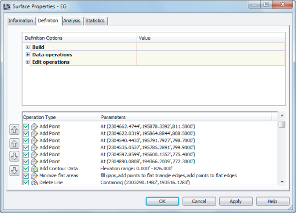
The most basic steps you can perform in making a better model are right in the Surface Properties dialog. The surface object contains information about the build and edit operations, along with some values used in surface calculations. These values can be used to tweak your surface to a semi-acceptable state before more manual operations are needed.
In this exercise, you'll go through a couple of the basic surface-building controls that are available. You'll use them one at a time in order to measure their effects on the final surface display.
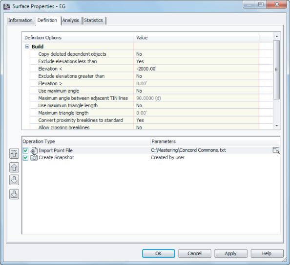
Figure 4.19 Surface Properties Definition Options
Save and keep the drawing open for the next portion of the exercise.
The Build options of the Definition tab allow you to tweak the way the triangulation occurs. The basic options are listed here:
Copy Deleted Dependent Objects
When you select Yes and an object (such as a surface boundary, breakline, or point group) that is part of the surface definition (such as the polylines you used in your aerial surface, for instance) is deleted, the information derived from that object is copied into the surface definition. Setting this option to Yes in the EG Surface Properties will let you erase the polylines from the drawing file while still maintaining the surface information. If this option is set to No for the EG surface, when the polylines (or any other drawing objects) are deleted they will be removed from the surface definition when the surface is rebuilt.
Exclude Elevations Less Than and Elevation <
Setting Exclude Elevations Less Than to Yes puts a floor on the surface. Any point that would be built into the surface but that is lower than the floor is ignored. In the EG surface, there are calculated boundary points with zero elevations, causing real problems that can be solved with this simple click. The floor elevation is controlled by the user by setting the Elevation < value.
Exclude Elevations Greater Than and Elevation >
The idea is the same as with the preceding options, but a ceiling value is used.
Use Maximum Angle and Maximum Angle Between Adjacent TIN Lines
These settings attempt to limit the number of narrow “sliver” triangles with one large obtuse angle and two acute angles that typically border a site. By not drawing any triangle with an angle greater than the user input value, you can greatly refine the TIN.
Use Maximum Triangle Length and Maximum Triangle Length
These settings attempt to limit the number of narrow “sliver” triangles that typically border a site. Similar to using a maximum angle, by not drawing any triangle with a length greater than the user input value, you can greatly refine the TIN.
Convert Proximity Breaklines To Standard
Toggling this option to Yes will create breaklines out of the lines and entities used as proximity breaklines. We will look at this more later.
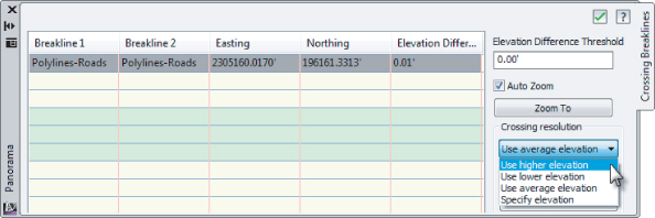
Allow Crossing Breaklines and Elevation To Use
These options specify what Civil 3D should do if two breaklines in a surface definition cross each other. An (x,y) coordinate pair cannot have two z values, so some decision must be made about crossing breaklines. If you set Allow Crossing Breaklines to Yes, you can then select whether to use the elevation from the first or the last breakline or to average these elevations.
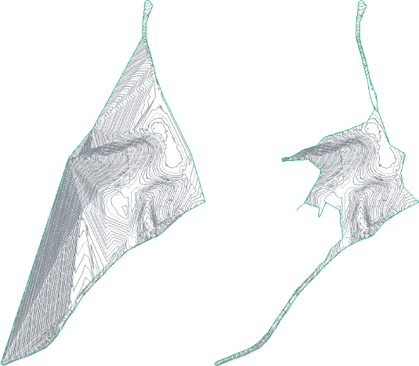
If you close the Surface Properties dialog and look at the surface, you might not notice the blob area shown in Figure 4.20. It appears that there are a series of blown shots, causing the elevation to dip to zero. In this next portion of the exercise, you'll limit the build options to make that blown surface “disappear.”
Figure 4.20 EG surface showing blown points

Figure 4.21 EG surface after ignoring low elevations

Figure 4.22 EG surface before Maximum Triangle (left) and after (right)
When this exercise is complete, you may close the drawing. A saved finished copy of this drawing is available from the book's web page with the filename SurfaceProperties _FINISHED.dwg or SurfaceProperties_METRIC_FINISHED.dwg.
The value is a bit high, but it is a good practice to start with a high value and work down to avoid losing any pertinent data. Setting this value to 225′ (or 70 m) will result in a surface that is acceptable because it doesn't lose a lot of important points. Beyond this, you'll need to look at making some edits to the definition itself instead of modifying the build options.
Surface Additions
Beyond the simple changes to the way the surface is built, you can look at editing the pieces that make up the surface. With your drawing so far, you have merely been building from points. Although this is fine for small surfaces, you need to go further with this surface. In this section, you'll add a few breaklines and a border and then perform some manual edits to your site.
![]()
Adding Breakline Information
Breaklines can come from any number of sources. They can be approximated on the basis of aerial photos of the site that help define surface features, or they can be directly input from field book files and the Civil 3D survey functionality. Five types of breaklines are available for use:
Standard Breaklines
Built on the basis of 3D lines, feature lines, or polylines, standard breaklines typically connect points already included in the surface definition but can contain their own elevation data. Simple-use cases for connecting the dots include linework from a survey or drawing a building pad to ensure that a flat area is included in the surface. Feature lines and 3D polylines are often used as the mechanism for grading design and include their own vertical information. An example might be the description of a parking lot perimeter or the invert of a V-shaped drainage swale.
Proximity Breaklines
These breaklines allow you to force triangulation without picking precise points. They will not add vertical information to the surface. The (x,y,z) coordinates will be based on the surface points in close proximity to the breakline.
Wall Breaklines
Wall breaklines define walls in surfaces. Because of the limitation of true vertical surfaces, a wall breakline will let you approximate a wall without having to create two separate breaklines. They are defined on the basis of an elevation at a vertex, and then an elevation difference at each vertex or for the full length of the breakline on a selected side. So a single wall breakline set with elevations will have the same result as creating a breakline with those same elevations and a second breakline that is vertically offset from the first.
From File Breaklines
You can select this option if a text file contains breakline information. This file can be the output of another program and can be used to modify the surface without creating additional drawing objects.
Non-destructive Breaklines
This type of breakline is designed to maintain the integrity of the original surface while updating triangulation. The (z) coordinate of the breaklines is calculated based on the surface creating new triangle vertexes to be formed.
In most cases, you'll build your surfaces from standard, proximity, and wall breaklines. In this example, you'll add in some breaklines that describe road and surface features:
Figure 4.23 The Add Breaklines dialog

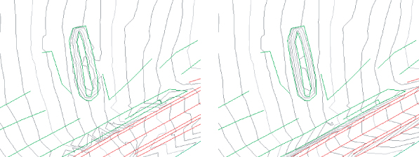
As shown in Figure 4.24, by adding the breaklines you force the TIN lines to align with the breaklines, thus cleaning up the contours and making them follow the ridgelines of the road centerline, gutterlines, and shoulders as well as the changes in grade around the small detention area.
Figure 4.24 EG surface with only contours displayed before breaklines added (left) and after (right)
When this exercise is complete, you may close the drawing. A saved finished copy of this drawing is available from the book's web page with the filename SurfaceBreaklines_FINISHED.dwg or SurfaceBreaklines_METRIC_FINISHED.dwg.
The surface changes reflect the breaklines added. On sites with more extreme grade breaks, such as those that might follow a channel or a site grading, breaklines are invaluable in building the correct surface.
Adding a Surface Boundary
In the previous exercise, you fixed some breakline issues. However, in the data presented, the bigger issue is still the number of inappropriate triangles that are being drawn along the edge of the site. It is often a good idea to leave these triangles untouched during the initial build of a surface, because they serve as pointers to topographical data (such as monumentation, control, utility information, and so on) that may otherwise go unnoticed. This is a common problem that can be solved by using a surface border. You can sketch in a polyline to approximate a border, but the Extract Objects from Surface utility gives you the ability to use the surface itself as a starting point.
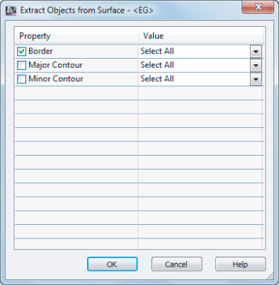
The Extract Objects from Surface utility allows you to re-create any displayed surface element (contours, border, etc.) as an independent AutoCAD entity. It is important to note that only the objects that are currently visible in the surface style are extractable. In this exercise, you'll extract the existing surface boundary as a starting point for creating a more refined boundary that will limit triangulation:
![]()
Figure 4.25 Extracting the border from the surface object
![]()
Figure 4.26 Using the grips to adjust the border
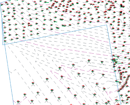
Figure 4.27 Revised surface border polyline
Outer Boundaries
Use this type to define the outer edge of the shown boundary. When the Non-destructive Breakline option is used, the points outside the boundary are still included in the calculations; then additional points are created along the boundary line where it intersects with the triangles it crosses. This boundary trims the surface for display but does not exclude the points outside the boundary. You'll want to have your outer boundary among the last operations in your surface-building process. Therefore, as future edits are made, you may want to move the Add Boundary build operation back to the bottom of the operations list on the Definition tab in the Surface Properties dialog, as discussed earlier in this chapter.
Show Boundaries
Use this type to show the surface inside a hide boundary, essentially creating a reverse donut effect in the surface display.
Hide Boundaries
Use this type to punch a hole in the surface display for tasks like building footprints or a wetlands area that are not to be touched by design. Hidden surface areas are not deleted but merely not displayed; therefore, the surface inside a hide boundary is still used for calculations such as area or cut/fill.
Data Clip Boundaries
Data clip boundaries place limits on data that will be considered part of the surface from that point going forward. This type is different from an outer boundary in that the data clip boundary will keep the data from ever being built into the surface as opposed to limiting it after the build. Using data clip boundaries is handy when you are attempting to build Civil 3D surfaces from large data sources such as Light Detection and Ranging (LiDAR) or DEM files. Because they limit data being placed into the surface definition, you'll want to have data clips among the first operations in your surface.
Figure 4.28 Add Boundaries dialog
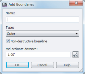
Figure 4.29 A non-destructive outer boundary in action
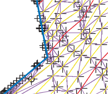
Figure 4.30 A destructive outer boundary in action
When this exercise is complete, you may close the drawing. A saved finished copy of this drawing is available from the book's web page with the filename SurfaceBoundary_FINISHED.dwg or SurfaceFromBoundary_METRIC_FINISHED.dwg.
As you have seen, the non-destructive boundary we looked at first is the peacekeeper. It always seeks to find a “common ground” (interpolated elevation) between the two existing points on either side of a TIN line that it crosses, whereas the destructive boundary is so powerful that it cuts off all communication between points inside and outside the boundary.
In spite of adding breaklines and a border, you still have some areas that need further correction or changes.
Surface Cropping
Surface cropping is useful when you are working with a small portion of a much larger surface. A cropped area within a surface becomes a separate surface object (a new surface) to be managed and manipulated on a much smaller scale. In this example, you will create a cropped surface and add it to an existing drawing:
![]()
Figure 4.31 The Create Cropped Surface dialog

Figure 4.32 The completed cropped surface

When this exercise is complete, you may close the drawing. A saved finished copy of this drawing with the cropped surface is available from the book's web page with the filename SurfaceCropping_FINISHED.dwg or SurfaceCropping_METRIC_FINISHED.dwg.
Manual Surface Edits
In your surface, you have a few “finger” surface areas where the surveyors went out along narrow paths from the main area of topographic data. The nature of TIN surfaces is to connect dots, and so these fingers often wind up as webbed areas of surface information that's not accurate or pertinent. A number of manual edits can be performed on a surface, including adding a boundary. These edit options are part of the definition of the surface and include the following:
Add Line
Connects two points where a triangle did not exist before. This option essentially adds a breakline to the surface, so adding a breakline would generally be a better solution. This option is not available on grid surfaces.
Delete Line
Removes the connection between two points. In addition to Outer Boundaries, this option is used frequently to clean up the edge of a surface or to remove internal data where a surface should have no triangulation at all. This can be an area such as a building pad or water surface.
Swap Edge
Changes the direction of the triangulation methodology. For any four points, there are two solutions to the internal triangulation, and the Swap Edge option alternates from one solution to the other. The necessity of numerous swap edge operations can be limited by the use of appropriate breaklines. This option is not available on grid surfaces.
Add Point
Allows for the manual addition of surface data. This function is often used to add a peak to a digitized set of contours that might have a flat spot at the top of a hill.
Delete Point
Allows for the manual removal of a data point from the surface definition. Generally, it's better to fix the source of the bad data, but this option can be a fix if the original data is not editable (in the case of a LandXML file, for example).
Modify Point
Modify Point allows for changing the elevation of a surface point. Only the TIN point is modified, not the original data input.
Move Point
Move Point is limited to horizontal movement. Like Modify Point, only the TIN point is modified, not the original data input. This option is not available on grid surfaces.
Minimize Flat Areas
Performs the edits you saw earlier in this chapter to add supplemental information to the TIN and to create a more accurate surface, forcing triangulation to work in the z direction instead of creating flat planes. This option is not available on grid surfaces.
Raise/Lower Surface
A simple arithmetic operation that moves the entire surface in the positive or negative z direction. This option is useful for testing rough grading schemes for balancing dirt or for adjusting entire surfaces after a new benchmark has been observed.
Smooth Surface
Presents a pair of methods for supplementing the surface TIN data (note that this option is not available on grid surfaces). Both smoothing methods work by extrapolating more information from the current TIN data, but they are distinctly different in their methodology:
Natural Neighbor Interpolation (NNI)
Adds points to a surface on the basis of the weighted average of nearby points. This data generally works well to refine contouring that is sharply angular because of limited information or long TIN connections. NNI works only within the bounds of a surface; it cannot extend beyond the original data.
Kriging
Adds points to a surface based on one of five distinct algorithms to predict the elevations at additional surface points. These algorithms create a trending for the surface beyond the known information and can therefore be used to extend a surface beyond even the available data. Kriging is very volatile, and you should understand the full methodology before applying this information to your surface. Kriging is frequently used in subsurface exploration industries such as mining, where surface (or strata) information is difficult to come by and the distance between points can be higher than desired.
Paste Surface
Pulls in the TIN information from the selected surface and replaces the TIN information in the host surface with this new information while keeping the dynamic relationship to the original surface. This option is helpful in creating composite surfaces that reflect both the original ground and the design intent. This option is not available on grid surfaces. We'll look at pasting in Chapter 16, “Grading.”
Simplify Surface
Allows you to reduce the amount of TIN data being processed while maintaining the accuracy of the surface. This is done using one of two methods: Edge Contraction, wherein Civil 3D tries to collapse two points connected by a line to one point, or Point Removal, which removes selected surface points based on algorithms designed to reduce data points that are similar. This option is not available on grid surfaces.
Manual editing should always be the last step in updating a surface. Fixing the surface is a poor substitution for fixing the underlying data the TIN is built from, but in some cases, it is the quickest and easiest way to make a more accurate surface.
Point and Triangle Editing
In this section, you'll remove triangles manually, and then finish your surface by correcting what appears to be a blown survey shot.
Figure 4.33 Using a Crossing Window selection

Figure 4.34 Surface before removal of extraneous triangles (left) and after (right)

When this exercise is complete, you may save and keep the drawing open to continue on to the next exercise or use the saved finished copy of this drawing available from the book's web page (SurfaceEdits_FINISHED.dwg or SurfaceEdits_METRIC_FINISHED.dwg).
Surface Smoothing
One common complaint about computer-generated contours is that they're simply too precise. The level of calculations in setting elevations on the basis of linear interpolation along a triangle leg makes it possible for contour lines to be overly exact, ignoring contour line trends in place of small anomalies of point information. Under the eye of a board drafter, these small anomalies were averaged out, and contours were created with smooth flowing lines.
While you can apply object-level smoothing as part of the contouring process, this process smooths the end result but not the underlying data. In this section, you'll use the NNI smoothing algorithm to reduce surface anomalies and create a more visually pleasing contour set:
Figure 4.35 Smooth Surface dialog

Figure 4.36 Surface before NNI smoothing (left) and after (right)
When this exercise is complete, you may close the drawing. A saved finished copy of this drawing is available from the book's web page with the filename SurfaceSmoothing_FINISHED.dwg or SurfaceSmoothing_METRIC_FINISHED.dwg.
Note that we said the surface will be smoothed — not the contours. Contour smoothing will be discussed later. To see the result of the surface smoothing, change Surface Style to Contours And Points to display your image as shown in Figure 4.37.
Figure 4.37 Points added via NNI surface smoothing
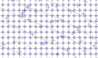
Note all of the points with a circle cross symbol. These points are all new, created by the NNI surface-smoothing operation. The derived points are part of your surface, and the contours reflect the updated surface information.
Surface Simplifying
Because of the increasing use in land development projects of GIS and other data-heavy inputs, it's critical that Civil 3D users know how to simplify the surfaces produced from these sources. In this exercise, you'll simplify the surface created from a drawing earlier in this chapter.
Figure 4.38 EG-GIS surface statistics before simplification

Figure 4.39 The Simplify Surface – Simplify Methods page

Figure 4.40 The Simplify Surface – Region Options page

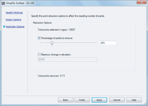
Figure 4.41 The Simplify Surface – Reduction Options page
When this exercise is complete, you may close the drawing. A saved finished copy of this drawing is available from the book's web page with the filename SurfaceSimplifying FINISHED.dwg or SurfaceSimplifying_METRIC_FINISHED.dwg.
A quick visit to the Surface Properties Statistics tab shows that the number of points has been reduced, as shown in Figure 4.42. On something like an aerial topography or DEM, reducing the point count probably will not reduce the usability of the surface, but this simple point reduction will decrease the file size. Remember, you can always delete the edit or deselect the operation on the Definition tab of the Surface Properties dialog to “un-simplify” the surface.
Figure 4.42 EG-GIS surface statistics after simplification

The creation of a surface is merely the starting point. Once you have a TIN to work with, you have a number of ways to view the data using analysis tools and varying styles.
Surface Analysis
![]()
Once a surface is created, you can display information in a number of ways. The most common so far has been contours and triangles, but those are the basics. By using varying styles, you can show a large amount of data with one single surface. Surface styles are discussed further in Chapter 21, “Object Styles.” While some of the styles are used for generating plans (such as contours), others lend themselves to analyzing the surface during creation.
For a surface object in plan view, Points, Triangles, Border, Major Contour, Minor Contour, User Contours, and Gridded are standard components and are controlled like any other object component. Directions, Elevations, Slopes, and Slope Arrows components are unique to surface styles. Note that the Layer, Color, and Linetype fields are grayed out for these components. Each of these components has its own special coloring schemes, which we'll look at in the next section. In this section, you will explore the elevation and slope analysis styles.
Elevation Banding
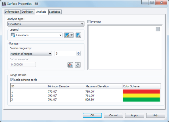
Displaying surface information as bands of color is one of the most common display methods for engineers looking to make a high-impact view of the site. Elevations are a critical part of the site design process, and understanding how a site varies in terms of elevation is an important part of making the best design. Elevation analysis typically falls into two categories: showing bands of information on the basis of pure distribution of linear scales or displaying a lesser number of bands to show some critical information about the site. In this first exercise, you'll use a standard style to illustrate elevation distribution along with a prebuilt color scheme that works well for presentations:
![]()
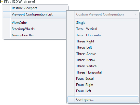

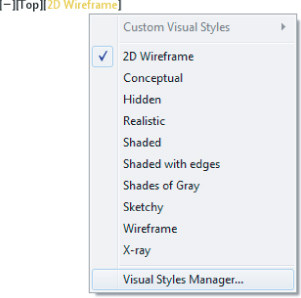
Figure 4.43 Conceptual view of the site with the Elevation Banding style
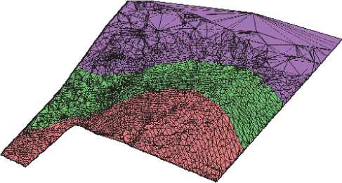
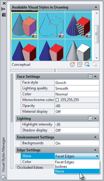
Figure 4.44 The Surface Properties dialog after manual editing
When this exercise is complete, you may close the drawing. A saved finished copy of this drawing is available from the book's web page with the filename SurfaceAnalysis_FINISHED.dwg or SurfaceAnalysis_METRIC_FINISHED.dwg.
Understanding surfaces from a vertical direction is helpful, but many times the slopes are just as important. In the next section, you'll take a look at using the slope analysis tools in Civil 3D.
Slopes and Slope Arrows
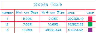
Beyond the bands of color that show elevation differences in your models, you also have tools that display slope information about your surfaces. This analysis can be useful in checking for drainage concerns, meeting accessibility requirements, or adhering to zoning constraints. Slope is typically shown as areas of color similar to the elevation banding or as colored arrows that indicate the downhill direction and slope. In this exercise, you'll look at a proposed site grading surface and run the two slope analysis tools:
![]()
Figure 4.45 The Slopes legend table
![]()
The benefit of arrows is in looking for “birdbath” areas that will collect water. These arrows can also verify that inlets are in the right location, as shown in Figure 4.46. Look for arrows pointing to the proposed drainage locations and you'll have a simple design-verification tool.
Figure 4.46 Slope arrows pointing to a proposed inlet location

When this exercise is complete, you may close the drawing. A saved finished copy of this drawing is available from the book's web page with the filename SlopeAnalysis_FINISHED.dwg or SlopeAnalysis_METRIC_FINISHED.dwg.
With these simple analysis tools, you can show a client the areas of their site that meet their constraints. Visually strong and simple to produce, this is the kind of information that a 3D model makes available. Beyond the basic information that can be represented in a single surface, Civil 3D also contains a number of tools for comparing surfaces. You'll compare this existing ground surface to a proposed grading plan in the next section.
Visibility Checker
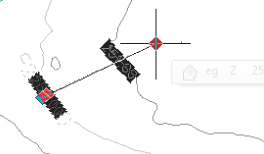
The Zone of Visual Influence tool allows you to explore what-if scenarios. In this example, a 40′ (12 m) tower has been proposed for the site. A concerned neighbor wants to make sure that it won't obstruct their scenic view. You want to check it from the proposed surface:
- Green near the tower location indicates that the object is completely visible.
- Yellow indicates that the object is partially visible.
- Red indicates that the object is not visible.
- If the arrow is green, it means that the view is unobstructed and the command line will tell you the distance from the eye.
- If any portion of the arrow is red, it indicates that the view is obstructed, and the command line will tell you the distance at which the obstruction occurs.
When this exercise is complete, you may close the drawing. A saved finished copy of this drawing is available from the book's web page with the filename SurfaceVisibility_FINISHED.dwg or SurfaceVisibility_METRIC_FINISHED.dwg.
Unfortunately, these visual tools are not dynamic; if you change the surface, you will need to rerun the visual tools. Perhaps this will be addressed in a future release.
Comparing Surfaces
Earthwork is a major part of almost every land development project. The money involved with earthmoving is a large part of the budget, and for this reason, minimizing this impact is a critical part of the final design. Civil 3D contains a number of surface analysis tools designed to help in this effort, and you'll look at them in this section. First, a simple comparison provides feedback about the volumetric difference, and then a more detailed approach enables you to perform an analysis on this difference.
For years, civil engineers have performed earthwork using a section methodology. Sections were taken at some interval, and a plot was made of both the original surface and the proposed surface. Comparing adjacent sections and multiplying by the distance between them yields an end-area method of volumes that is generally considered acceptable. The main problem with this methodology is that it ignores the surfaces in the areas between sections. These areas could include areas of major change, introducing some level of error. In spite of this limitation, this method worked well with hand calculations, trading some accuracy for ease and speed.
With the advent of full-surface modeling, more precise methods became available. By analyzing both the existing and proposed surfaces, a volume calculation can be performed that is as good as the two surfaces. At every TIN vertex in both surfaces, a distance is measured vertically to the other surface. These delta amounts can then be used to create a third dynamic surface called a volume surface, which represents the difference between the two original surfaces.
TIN Volume Surface
Using the volume utility for initial design checking is helpful, but quite often contractors and other outside users want to see more information about the grading and earthwork for their own uses. This requirement typically falls into two categories: a cut-fill analysis showing colors or contours or a grid of cut-fill tick marks.
Color cut-fill maps are helpful when reviewing your site for the locations of movement. Some sites have areas of better material or can have areas where the cost of cut is prohibitive (such as rock). In this exercise, you'll use two of the surface analysis methods to look at the areas for cut-fill on your site:
![]()
![]()
Figure 4.47 Creating a volume surface
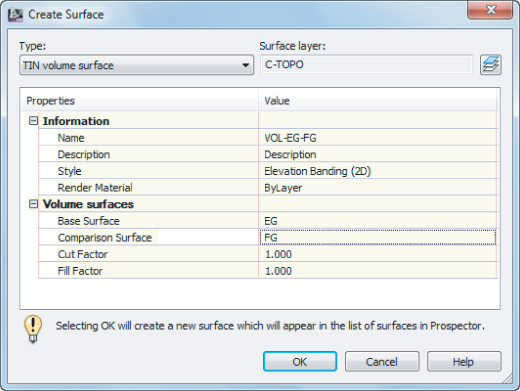
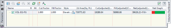
Figure 4.48 Composite volume calculated
![]()
Figure 4.49 Elevation analysis settings for earthworks
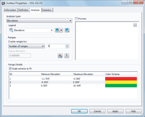
Figure 4.50 Completed elevation analysis

![]()
- Shades of red for cut
- A yellow for the balance line
- Shades of green for fill
![]()
When this exercise is complete, you may close the drawing. A saved finished copy of this drawing is available from the book's web page with the filename VolumeSurface_FINISHED.dwg or VolumeSurface_METRIC_FINISHED.dwg.
The volume surface can now be analyzed on a lot-by-lot basis or labeled using the surface-labeling functions to show the depths of cut and fill, which you'll look at in the next sections.
Labeling the Surface
![]()
Once the three-dimensional surface model has been created, it is time to communicate the model's information in various formats. This includes labeling contours, creating legends for the analysis you've created, adding spot labels, or labeling the slope. These exercises work through these main labeling requirements and building styles for each.
Contour Labeling
The most common requirement is to place labels on surface-generated contours. In Land Desktop, this was one of the last steps because a change to a surface required erasing and replacing all the labels. Once labels have been placed, their styles can be modified.
Contour labels in Civil 3D are created by special lines that understand their relationship with the surface. Everywhere one of these lines crosses a contour line, a label is placed. This label's appearance is based on the style applied and can be a major, minor, or user-defined contour label. Each label can have styles selected independently, so using some AutoCAD selection techniques can be crucial to maintaining uniformity across a surface. In this exercise, you'll add labels to your surface and explore the interaction of contour label lines and the labels themselves.
Figure 4.51 Contour labels applied

Figure 4.52 Grip-editing a contour label line
By using the created label lines instead of adding new ones, you'll find it easier to manage the layout of your labels.
Surface Point Labels
In every site, there are points that fall off the contour line but are critical. In an existing surface, this can be the low point in a swale or a driveway that has to be matched. When you're working with a paper set of plans, the spot grade is the most common review element. One of the most time-consuming issues in land development is the preparation of grading plans with hundreds of individual spot grades. Every time a site grading scheme changes, these were typically updated manually, leaving lots of opportunities for error.
With Civil 3D's surface modeling, spot labels are dynamic and react to changes in the underlying surface. By using surface labels instead of points or text callouts, you can generate a grading plan early on in the design process and begin the process of creating sheets. In this section, you'll label surface slopes in a couple of ways, create a single spot label for critical information, and conclude by creating a grid of labels similar to many estimation software packages.
Labeling Slopes
Beyond the specific grade at any single point, most grading plans use slope labels to indicate some level of trend across a site or drainage area. Civil 3D can generate the following two slope labels:
One-Point Slope Labels
One-point slope labels indicate the slope of an underlying surface triangle. These work well when the surface has large triangles, typically in pad or mass grading areas.
Two-Point Slope Labels
Two-point slope labels indicate the slope trend on the basis of two points selected and their locations on the surface. A two-point slope label works by dividing the surface elevation distance between the points by the planar distance between the pick points. This works well in existing ground surface models to indicate a general slope direction but can be deceiving in that it does not consider the terrain between the points.
In this next exercise, you'll apply both types of slope labels, and then look at a minor style modification that is commonly requested:
Figure 4.53 A one-point slope label

Figure 4.54 A two-point slope label
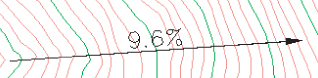
This second label indicates the average slope of the property. By using a two-point label, you get a better understanding of the trend, as opposed to a specific point.
When this exercise is complete, you may close the drawing. A saved finished copy of this drawing is available from the book's web page with the filename SurfaceLabeling_FINISHED.dwg or SurfaceLabeling_METRIC_FINISHED.dwg.
Critical Points
A typical grading plan is a sea of critical points that drive the site topography. In the past, much of this labeling and point work was done by creating coordinate geometry (COGO) points and simply displaying their properties. Although this is effective, it has two distinct disadvantages. First, these points are not reflective of the design but part of the design. This makes the sheet creation a part of the grading process, not a parallel process. Second, the addition of COGO points to any drawing and project when they're not truly needed just weighs down the design model. Point management is a mentally intensive task, and anything that can limit extraneous data is worth investigating.
Surface labels react dynamically to the surface and to the point of insertion. Moving any of these labels would update the information to reflect the surface underneath. This relationship makes it possible for one user to place labels on a grading plan while the final surface is still in flux. A change in the proposed surface is reflected in an update from the project, and an updated sheet can be on the plotter in minutes.
Surface Grid Labels
Sometimes, more than a few points are requested. Estimation software typically creates a grid of point labels that can be easily reviewed or passed to a contractor for fieldwork. In this exercise, you'll use the volume surface you generated earlier in this chapter to create a set of surface labels that reflect this requirement:
Wait a few moments as Civil 3D generates all the labels just specified. Your drawing should look similar to Figure 4.55.
Figure 4.55 Volume surface with grid labels

Labeling the grid is imprecise at best. Grid labeling ignores anything that might happen between the grid points, but it presents the surface data in a familiar way for engineers and contractors. By using the tools available and the underlying surface model, you can present information from one source in an almost infinite number of ways.
When this exercise is complete, you may close the drawing. A saved finished copy of this drawing is available from the book's web page with the filename SurfaceVolumeGridLabels_FINISHED.dwg or SurfaceVolumeGridLabels_METRIC_FINISHED.dwg.
Point Cloud Surfaces
A point cloud is a huge bunch of 3D points, usually collected by laser scanner or Light Detection and Ranging (LiDAR). In a geographic information system (GIS), point clouds are often used as a source for a Digital Elevation Model (DEM). The technology has gotten less expensive and more accurate over the last few years, allowing LiDAR to quickly take over from traditional methods of collecting photogrammetry data.
Point clouds in many formats can be imported to Civil 3D. The most common format is the Log ASCII Standard (LAS) file. This binary format is a public format and at minimum contains x, y, and z data. LAS data can also include the following:
- Coordinate system of scanned area.
- Color — true color on RGB format.
- Intensity; LiDAR depends on lasers bouncing off objects and back to the scanning device and the intensity refers to the strength of the returned information. This value directly relates to the material from which the laser is bouncing. For example, concrete will have a stronger intensity than grass.
- Classification, which will be a number, most frequently between 0 and 9, that categorizes points based on material (i.e., ground, vegetation, or buildings).
For more information on the LAS standard, visit www.asprs.org.
Civil 3D can import a point cloud and use it in several ways. For instance, a laser scan of a bridge can be imported and placed for reference when designing a road through an existing abutment. In the example that follows, you will convert LiDAR data into a Civil 3D surface. It is important to note that point clouds often contain millions of points and require a beefy computer (and a little patience on your part) to process.
Importing a Point Cloud
A typical point cloud contains millions of points. These large files are kept external to Civil 3D in a point cloud database. After the LAS has been imported, the data is passed to three files: PRMD, IATI, and ISD. The ISD file contains the points themselves and is the only file needed by CAD if the point cloud would need to be re-created or used in base AutoCAD. By default these files get created in the same directory as the DWG but can be changed when importing the information.
If the point cloud you are working with contains coordinate system information (as all the examples in this book do), the software will automatically convert the point cloud to the units and coordinate system of the drawing. For the exercises in this chapter, it does not matter whether you choose the Metric or the Imperial template.
Civil 3D may take a long time to process these files, and you must ensure you have sufficient disk space to store them, as you will find in the following exercise. It is also a good idea to close the software and then reopen it to help clear some memory before starting memory-intensive tasks such as working with point clouds. The following exercise will show you how to import and work with a point cloud:
Figure 4.56 Create Point Cloud – Information page
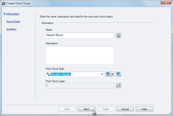
Figure 4.57 The Create Point Cloud – Source Data page

Figure 4.58 The Create Point Cloud – Summary page
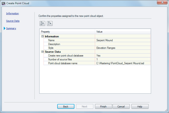
When complete, a portion of a bounding box outlining a portion of the point cloud is displayed in the center of the screen. Save the drawing but leave it open to complete the next exercise.
Working with Point Clouds
Once the point cloud is visible in your drawing, you'll want to follow a few rules of thumb to prevent performance problems. The key-in POINTCLOUDDENSITY value controls what percentage of the full point cloud displays on the screen at once. You can also access this value using a slider bar in the Point Cloud contextual tab. However, it is easier to hit the percentage you want on the first try if you use the key-in value. The lower this value, the fewer points are visible; hence the easier it will be to navigate your drawing. The POINTCLOUDDENSITY value does not have any effect on the number of points used when generating a surface model (this is similar to the Level Of Detail value used to aid surface processing).
When you are changing view directions on a point cloud, we recommend that you use preset views and named views to flip around the object. The orbit commands should not be used, as they are a surefire way to max out your computer's RAM. If you used the default template, your surface will be located on the V-SITE-SCAN layer. We suggest that you freeze the layer if you do not need to see the point cloud. Use Freeze instead of Off for layer management so the point cloud is not accounted for during pan, zoom, and regen operations (this is true for all AutoCAD objects, but it makes a huge difference when working with point clouds).
Creating a Point Cloud Surface
By specifying either an entire point cloud or a small region of a point cloud, you can create a new TIN surface in your drawing. Any changes to the point cloud object will render the surface definition out of date. In the following exercise, a new TIN surface is created from the point cloud previously imported:
Figure 4.59 The Point Cloud contextual tab
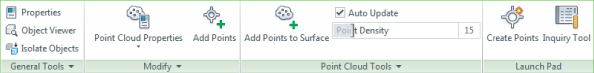
Figure 4.60 The Add Points To Surface – Surface Options page

Figure 4.61 The Add Points To Surface – Region Options page
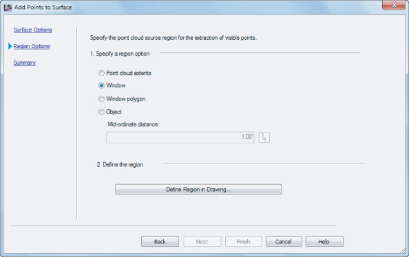
Figure 4.62 The Add Points To Surface – Summary page

When this exercise is complete, you may close the drawing. Due to the large file size, a finished state of this drawing is not available for download.
The Bottom Line
Create a preliminary surface using freely available data.
Most land development projects involve a surface at some point. During the planning stages, freely available data can give you a good feel for the lay of the land, allowing design exploration before money is spent on fieldwork or aerial topography. Imprecise at best, this free data should never be used as a replacement for final design topography, but it's a great starting point.
Master It
Create a new drawing from the Civil 3D template and set the Coordinate System to NAD83 Connecticut State Plane Zone, US Foot (CT83F) or NAD83 Connecticut State Plane Zone, Meter (CT83). Create a surface named MarlboroughCT_DEM. Add the Marlborough_CT.DEM file (UTM Zone 18, NAD27 datum, meters) downloadable from the book's web page.
Modify and update a TIN surface.
TIN surface creation is mathematically precise, but sometimes the assumptions behind the equations leave something to be desired. By using the editing tools built into Civil 3D, you can create a more realistic surface model.
Master It
Open the MasteringBoundary.dwg or the MasteringBoundary_METRIC.dwg file. Use the irregular-shaped polyline and apply it to the surface as an outer boundary of the surface.
Prepare a slope analysis.
Surface analysis tools allow users to view more than contours and triangles in Civil 3D. Engineers working with nontechnical team members can create strong meaningful analysis displays to convey important site information using the built-in analysis methods in Civil 3D.
Master It
Open the MasteringSlopeAnalysis.dwg or the MasteringSlopeAnalysis_METRIC.dwg file. Create a Slope Banding analysis showing slopes under and over 10 percent and insert a legend to help clarify the image.
Label surface contours and spot elevations.
Showing a stack of contours is useless without context. Using the automated labeling tools in Civil 3D, you can create dynamic labels that update and reflect changes to your surface as your design evolves.
Master It
Open the MasteringLabelSurface.dwg or the MasteringLabelSurface_METRIC.dwg file. Label the major contours on the surface at 2′ and 10′ (Background) or 1 m and 5 m (Background).
Import a point cloud into a drawing and create a surface model.
As point cloud data becomes more common and replaces other large-scale data-collection methods, the ability to use this data in Civil 3D is critical. Intensity helps postprocessing software determine the ground cover type. While Civil 3D can't do postprocessing, you can see the intensity as part of the point cloud style.
Master It
Import an LAS format point cloud Denver.las into the Civil 3D template (with a coordinate system) of your choice. As you create the point cloud file, set the style to Elevation Ranges. Use a portion of the file to create a Civil 3D surface model.