CHAPTER 12
Maya Dynamics and Effects
Special effects animations simulate not only physical phenomena, such as smoke and fire, but also the natural movements of colliding bodies. Behind the latter type of animation is the Maya dynamics engine, which is the sophisticated software that creates realistic-looking motion based on the principles of physics.
Another powerful Maya animation tool, Paint Effects, can create dynamic fields of grass and flowers, a head full of hair, and other such systems in a matter of minutes. Maya also offers dynamic simulations for hair, fur, and cloth. In this chapter, we'll cover the basics of dynamics in Maya and let you practice working with particles by making steam.
Topics in this chapter include:
- An overview of dynamics and Maya Nucleus
- Rigid and soft dynamic bodies
- Animating with dynamics: the pool table
- nParticle dynamics
- Emitting nParticles
- Animating an nParticle effect: locomotive steam
- Introduction to Paint Effects
- Customizing Maya
- Where do you go from here?
An Overview of Dynamics and Maya Nucleus
Dynamics is the simulation of motion through the application of the principles of physics. Rather than assigning keyframes to objects to animate them, with Maya dynamics you assign physical characteristics that define how an object behaves in a simulated world. You create the objects as usual in Maya, and then you convert them to dynamic bodies. Dynamic bodies are defined through dynamic attributes you add to them, which affect how the objects behave in a dynamic simulation.
Dynamic bodies are affected by external forces called fields, which exert a force on them to create motion. Fields can range from wind forces to gravity and can have their own specific effects on dynamic bodies.
In Maya, dynamic objects are categorized as bodies, particles, hair, and fluids. Dynamic bodies are created from geometric surfaces and are used for physical objects such as bouncing balls. Particles are points in space that have renderable properties and are used for numerous effects, such as fire and smoke. We'll cover particle basics in the latter half of this chapter. Hair consists of curves that behave dynamically, such as strings. Fluids are, in essence, volumetric particles that can exhibit surface properties. You can use fluid dynamics for natural effects such as billowing clouds or plumes of smoke.
Nucleus is a more stable and interactive way of calculating dynamic simulations in Maya than its traditional dynamics engine. Nucleus speeds up the creation and increases the stability of some dynamic effects in Maya, including particle effects and cloth simulation (through nCloth).
In the Maya 2009 release, Autodesk introduced nParticles. They're closely related to traditional particles in Maya but have been made easier to create and manage, requiring less explicit expression controls than before.
We'll introduce nParticles (instead of traditional particles) later in this chapter; however, soft bodies, hair, nCloth, and fluid dynamics are advanced topics and won't be covered in this book.
Rigid and Soft Dynamic Bodies
The two types of dynamic bodies are rigid and soft. Rigid bodies are solid objects, such as a pair of dice or a baseball, that move and rotate according to the dynamics applied. Fields and collisions affect the entire object and move it accordingly. Soft bodies are malleable surfaces that deform dynamically, such as drapes in the wind or a bouncing rubber ball. In brief, this is accomplished by making the surface points (NURBS, CVs, or polygon vertices) of the soft body object dynamic instead of the whole object. The forces and collisions of the scene affect these surface points, making them move to deform their surface. In this section, you'll learn about rigid body dynamics.
Creating Active and Passive Rigid Body Objects
Any surface geometry in Maya can be converted to a rigid body. After it's converted, that surface can respond to the effects of fields and take part in collisions. Sounds like fun, eh?
The two types of rigid bodies are active and passive. An active rigid body is affected by collisions and fields. A passive rigid body isn't affected by fields and remains still when it collides with another object. A passive rigid body is used as a surface against which active rigid bodies collide.
The best way to see how the two types of rigid bodies behave is to create some and animate them. In this section, you'll do that in the classic animation exercise of a bouncing ball.
To create a bouncing ball using Maya rigid bodies, switch to the Dynamics menu and follow these steps:
- Create a polygonal plane, and scale it to be a ground surface.
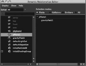
- Create a poly sphere, and position it a number of units above the ground, as shown in Figure 12.1.
- Make sure you're in the Dynamics menu set (choose Dynamics from the Status Line drop-down bar). Select the poly sphere, and choose Soft/Rigid Bodies
 Create Active Rigid Body. The sphere's Translate and Rotate attributes turn yellow. There will be a dynamic input for those attributes, and as such, you can't set keyframes on any of them.
 - Select the ground plane, and choose Soft/Rigid Bodies Create Passive Rigid Body. Doing so sets the poly plane as the floor. For this exercise, stick with the default settings and ignore the various creation options and Rigid Body attributes.
- To put the ball into motion, you need to create a field to affect it. Select the sphere, and choose Fields Gravity. By selecting the active rigid object(s) while you create the field, you connect that field to the objects automatically. Fields affect only the active rigid bodies to which they're connected. If you hadn't established this connection initially, you could still do so later, through the Dynamic Relationships Editor. You'll find out more about this process later in this chapter.
Figure 12.1 Place a poly sphere a few units above a poly plane ground surface.

If you try to scrub the timeline, you'll notice that the animation doesn't run properly. Because dynamics simulates physics, no keyframes are set. You must play the scene from start to finish for the calculations to execute properly. You must also play the scene using the Play Every Frame option. Click the Animation Options button to the right of the Range slider, or choose Window ![]() Settings/Preferences
Settings/Preferences ![]() Preferences. In the Preferences window, choose Time Slider under the Settings header. Choose Play Every Frame from the Playback Speed menu. You can also set the maximum frames per second that your scene will play back by setting the Max Playback Speed attribute.
Preferences. In the Preferences window, choose Time Slider under the Settings header. Choose Play Every Frame from the Playback Speed menu. You can also set the maximum frames per second that your scene will play back by setting the Max Playback Speed attribute.
To play back the simulation, set your frame range from 1 to at least 500. Go to frame 1, and click Play. Make sure you have the proper Playback Speed settings in your Preferences window; otherwise, the simulation won't play properly.
When the simulation plays, you'll notice that the sphere begins to fall after a few frames and collides with the ground plane, bouncing back up.
As an experiment, try turning the passive body plane into an active body using the following steps:
- Select the plane, and open the Attribute Editor.
- In the rigidBody2 tab, select the Active check box. This switches the plane from a passive body to an active body.
- Play the simulation. The ball falls to hit the plane and knock it away. Because the plane is now an active body, it's moved by collisions. But because it isn't connected to the gravity field, it doesn't fall with the ball.
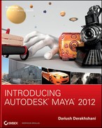
To connect the now-active body plane to the gravity field, open the Dynamic Relationships Editor window, shown in Figure 12.2 (choose Window ![]() Relationship Editors
Relationship Editors ![]() Dynamic Relationships).
Dynamic Relationships).
On the left is an Outliner list of the objects in your scene. On the right is a list from which you can choose a category of objects to list: Fields (default), Collisions, Emitters, or All. Select the geometry (pPlane1) on the left side, and then connect it to the gravity field by selecting the gravityField1 node on the right.
Figure 12.2 The Dynamic Relationships Editor window
When you connect the gravity field to the plane and run the simulation, you'll see the plane fall away with the ball. Because the two fall at the same rate (the rate set by the single gravity field), they don't collide. To disconnect the plane from the gravity field, deselect the gravity field in the right panel.
You can also connect a dynamic object to a field by selecting the dynamic object or objects and then the desired field and choosing Fields ![]() Affect Selected Object(s). This method is more useful for connecting multiple dynamic objects to a field.
Affect Selected Object(s). This method is more useful for connecting multiple dynamic objects to a field.
Turning the active body plane back to a passive floor is as simple as returning to frame 1, the beginning of the simulation, and clearing the Active attribute in the Attribute Editor. By turning the active body back to a passive body, you regain an immovable floor upon which the ball can collide and bounce.
RELATIONSHIP EDITORS
The Relationship Editors, such as the Dynamic Relationships window, are a means to connect two nodes to create a special relationship. The Dynamic Relationships Editor window specializes in connecting dynamic attributes so that fields, particles, and rigid bodies can interact in a simulation. Another example of a Relationship Editor is the Light Linking window, which allows you to connect lights to geometry so that they light only that specific object or objects. These are fairly advanced topics; however, as you learn more about Maya, their use will become integral in your workflow.
Moving a Rigid Body
Because Maya's dynamics engine controls the movement of any active rigid bodies, you can't set keyframes on their translation or rotation. With a passive object, however, you can set keyframes on translation and rotation as you can with any other Maya object. You also can easily keyframe an object to turn either active or passive.
Any movement that the passive body has through regular keyframe animation is translated into momentum, which is passed on to any active rigid bodies with which the passive body collides. Think of a baseball bat that strikes a baseball. The bat is a passive rigid body that you have keyframed to swing. The baseball is an active rigid body that is hit by (collides with) the bat as it swings. The momentum of the bat is transferred to the ball, and the ball is sent flying into the stadium stands. You'll see an example of this in action in the next exercise.
Rigid Body Attributes
Here is a rundown of the more important attributes for both passive and active rigid bodies as they pertain to collisions:
Mass Sets the relative mass of the rigid body. Set on active or passive rigid bodies, mass is a factor in how much momentum is transferred from one object to another. A more massive object pushes a less massive one with less effort and is itself less prone to movement when hit. Mass is relative, so if all rigid bodies have the same mass value, there is no difference in the simulation.
Static and Dynamic Friction Sliders Set how much friction the rigid body has while at rest (static) and while in motion (dynamic). Friction specifies how much the object resists moving or being moved. A friction of 0 makes the rigid body move freely, as if on ice.
Bounciness Specifies how resilient the body is upon collision. The higher the bounciness value, the more bounce the object has upon collision.
Damping Creates a drag on the object in dynamic motion so that it slows down over time. The higher the damping, the more the body's motion diminishes.
Animating with Dynamics: The Pool Table
This exercise will take you through the creation of a scene in which you'll use dynamics to animate a cue ball striking two balls on a pool table.
Creating the Pool Table and the Balls
You'll create a simple pool table as a collision surface for the pool balls. To create the table, follow these steps:
- Create a polygonal plane for the surface of the table. Scale it to 10 along its height and length.
- To create the pocket holes, make two holes in opposite corners. The easiest way is to duplicate the tabletop plane and offset it slightly in both directions, as shown in Figure 12.3. Doing so creates a pair of square holes in the corners for the ball to drop through. For this exercise, it will do perfectly well.
Figure 12.3 Duplicate the tabletop plane, and offset it slightly in both directions.
- Create a polygonal cube, and scale it to fit one edge of the plane to create a rail. Duplicate the cube three times, and then move and rotate the pieces to create the rails around the table, as shown in Figure 12.4.
Figure 12.4 A simple pool table

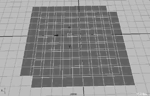
- Create three poly spheres, and then scale and place them as shown in Figure 12.5. It's important to place them slightly above the pool table surface. Although it's not imperative to have the exact location shown in the figure, it's a good idea to get close to the layout shown.
Figure 12.5 Scaling and placing the three spheres
- Shade your pool balls to make each one different. The figures in this exercise show a solid white ball, a striped ball (it will be yellow on your screen), and a black eight ball, as shown in Figure 12.6.
Figure 12.6 The pool balls in Texture view
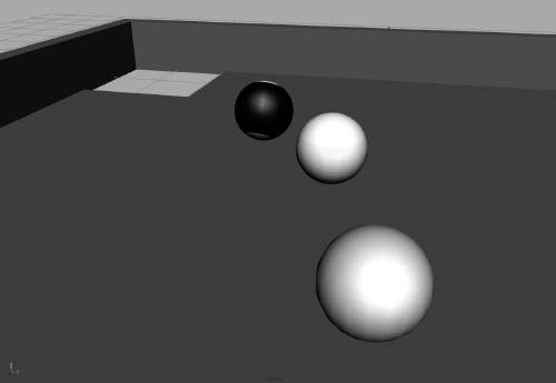
The spheres are placed a bit over the table surface so that their geometries' surfaces aren't accidentally crossing each other, an effect known as interpenetrating. When surfaces interpenetrate, the dynamics that result are usually as welcome as sand in your eyes. Starting all colliding rigid bodies slightly away from each other should guarantee that their surfaces don't interpenetrate. Using the simple pool table that you've set up will make the dynamics calculations quick and easy.
Use the file Table_v1.mb in the Scenes folder of the Pool_Table project on the book's companion web page, www.sybex.com/go/intromaya2012, as a reference or to catch up to this point.
Creating Rigid Bodies
Define the pool table as a passive rigid body, and define the pool balls as active rigid bodies. Follow these steps:
- Select the two planes that make up the tabletop and the four cubes that are the side rails. Choose Soft/Rigid Bodies Create Passive Rigid Body.
- Select the three balls, and choose Soft/Rigid Bodies Create Active Rigid Body to make them active rigid bodies.
- With all three pool balls selected, create a gravity field by choosing Fields Gravity. The gravity field automatically connects to all three balls.
- Run the simulation. You should see the balls fall slightly onto the tabletop. Check to see that none of them interpenetrate the table surface. If any of them do, Maya will select the offending geometry and display an error message in the Command Feedback line, turning it red.
Animating Rigid Bodies
If you need to, enable Texture view in your view panel by pressing 6.
The next step is to put the cue ball (the white sphere) into motion so that it hits the striped ball into the black eight ball to sink it into the corner pocket. Keyframe the cue ball's translation from its starting point to hit into the striped ball. However, because active rigid bodies can't be keyframed, you have to turn the cue ball into a passive rigid body. To do that, follow these steps:
- Select the cue ball (the white ball). Notice the Active attribute in the Channel Box. (You may have to scroll down; it's at the bottom.) It's set to On.
- Rewind your animation to the first frame. Choose Soft/Rigid Bodies Set Passive Key. Notice that the Active attribute turns a dark yellow. You've set a keyframe for the active state of the cue ball, and it now says Off. You can toggle rigid bodies between passive and active. Maya has also set translation and rotation keyframes for the cue ball.
- Go to frame 10. Move the cue ball with the Translate tool so that its outer surface slightly passes through the yellow-striped ball, as shown in Figure 12.7. Choose Soft/Rigid Bodies Set Passive Key.
Figure 12.7 Move the cue ball with the Translate tool.
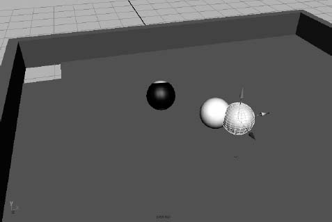
- Go to frame 11, and choose Soft/Rigid Bodies Set Active Key. This turns the cue ball back into an active rigid body in the frame after it strikes the striped ball.
By animating the ball as a passive rigid body, keyframing its translation, and then turning it back to active, you set the dynamic simulation in motion. The cue ball animates from its starting position and hits the striped ball. Maya's dynamics engine calculates the collisions on that ball and sets it into motion; the ball then strikes the black eight ball, which should roll into the corner pocket. The dynamics engine, at frame 11, also calculates the movement of the cue ball after it strikes the striped ball, so you don't have to animate its ricochet.
Go to the start frame, and play back the simulation. The cue ball knocks the striped ball into the eight ball. The eight ball rolls into the corner, and the striped ball bounces off to the right. If the eight ball doesn't go into the corner, you'll have to edit your cue ball's keyframes to hit the striped ball at the correct angle to hit the eight ball into the corner pocket.
At the current settings, however, the eight ball bounces out of the corner without falling through the hole. You need to control the bounciness of the collisions:
- Go back to the first frame. Select all three balls. In the Channel Box, change the Bounciness attribute from 0.6 to 0.2. After you set the attribute value in the Channel Box, Maya sets the value for all three spheres concurrently.
Changing the Bounciness attribute through the Attribute Editor changes the value for only one sphere even when they're all selected. You have to change the value for each sphere individually in the Attribute Editor. This is true for all values changed on multiple objects through the Attribute Editor.
- Play back the animation, and you'll see that the balls don't ricochet off each other and the sides of the pool table with as much spring. The eight ball should now fall through the hole. (See Figure 12.8.) You may need to increase your frame range if your ball doesn't quite make it by frame 120; try 200 frames instead.
You can download the scene file Table_v2.mb from the Pool_Table project on the web page to compare your work.
Figure 12.8 The eight ball falls through the hole.

Additional Rigid Body Attributes
In addition, while using the pool table setup without any animation, try playing with the rigid body attributes to see how they affect the rigid body in question. Some of these attributes are defined here:
Initial Velocity Gives the rigid body an initial push to move it in the corresponding axis.
Initial Spin Gives the rigid body object an initial twist to start the rotation of the object in that axis.
Impulse Position Gives the object a constant push in that axis. The effect is cumulative; the object will accelerate if the impulse isn't turned off.
Spin Impulse Rotates the object constantly in the desired axis. The spin will accelerate if the impulse isn't turned off.
Center of Mass (0,0,0) Places the center of the object's mass at its pivot point, typically at its geometric center. This value offsets the center of mass, so the rigid body object behaves as if its center of balance is offset, like trick dice or a top-weighted ball.
Creating animation with rigid bodies is straightforward and can go a long way toward creating natural-looking motion for your scene. Integrating such animation into a final project can become fairly complicated, though, so it's prudent to become familiar with the workings of rigid body dynamics before relying on that sort of workflow for an animated project. You'll find that most professionals use rigid body dynamics as a springboard to create realistic motion for their projects. The dynamics are often converted to keyframes and further tweaked by the animator to fit into a larger scene.
Here are a few suggestions for scenes using rigid body dynamics:
Bowling Lane The bowling ball is keyframed as a passive object until it hits the active rigid pins at the end of the lane. This scene is simple to create and manipulate.
Dice Active rigid dice are thrown into a passive rigid craps table. This exercise challenges your dynamics abilities as well as your modeling skills if you create an accurate craps table.
Game of Marbles This scene challenges your texturing and rendering abilities as well as your dynamics abilities.
Baking Out a Simulation
Frequently, a dynamic simulation is created to fit into another scene, perhaps to interact with other objects and such. In instances such as this, you want to exchange the dynamic properties of the dynamic body you have set up in a simulation for regular, good old-fashioned animation curves that you can edit along with the rest of the animated scene, if need be. You can easily take a simulation that you've created and bake it out to curves. As much fun as it is to think of cupcakes, baking is a somewhat catchall term used to describe converting one type of action or procedure into another; in this case, you're baking dynamics into keyframes.
You'll take the simulation you set up with the pool balls earlier and turn them into keyframes to give you a quick idea of how it can be done and the curves that you'll get. Dynamics is a deep layer of Maya, and there is a lot to learn about it. Keep in mind that you can use this introduction as a foundation for your own explorations.
To bake out the rigid body simulation of the pool balls, follow these steps:
- Open the scene file Table_v2.mb from the Pool_Table project on the web page, or if you prefer, open your scene from the previous exercise.
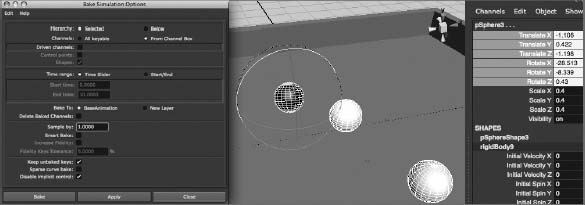
- Select all three pool balls, and choose Edit Keys Bake Simulation
 . In the option box, shown in Figure 12.9, set Time Range to Time Slider (which should be set to 1 to 150). This, of course, sets the range you would like to bake into curves.
 - Set Hierarchy to Selected, and set Channels to From Channel Box. This ensures that you have control over which keys are created. Make sure Keep Unbaked Keys and Disable Implicit Control are checked and that Sparse Curve Bake is turned off. Before clicking the Bake or Apply button, select the Translate and Rotate channels in the Channel Box. Click Bake.
- Maya runs through the simulation. Scrub the timeline back and forth. Notice how the pool balls move around normally as if the dynamic simulation were running—except that you can scrub in the timeline, which you can't do with a dynamics simulation. If you open the Graph Editor, you'll see something similar to Figure 12.10.
- The curves are crowded; they have keyframes at every frame. A typical dynamics bake gives results like this. But you can set the Bake command to sparse the curves for you; that is, it can take out keyframes at frames that have values within a certain tolerance, so that a minor change in the ball's position or rotation need not have a keyframe on the curve.
Figure 12.9 The Bake Simulation Options window
- Let's go back in time and try this again. Press Z (Undo) until you back up to right before you baked out the simulation to curves. You can also close this scene and reopen it from the original project, if necessary. This time, select the balls, and choose Edit Keys Bake Simulation . In the option box, turn on the Sparse Curve Bake setting, and set Sample By to 5. Select the channels in the Channel Box, and click Bake. You're telling Maya to only look at every five frames of the simulation to set keyframes.
- Maya runs through the simulation again and bakes everything out to curves. This time it makes a sparser animation curve for each channel because it's looking at five-frame intervals, as shown in Figure 12.11. If you open the Graph Editor, you'll notice that the curves are much friendlier to look at and edit.
Figure 12.10 The pool balls have animation curves.

Figure 12.11 Sampling by fives makes a cleaner curve.

Sampling by fives may give you an easier curve to edit, but it can oversimplify the animation of your objects; make sure you use the best Sampling setting for your simulation when you need to convert it to curves for editing.
Simplifying Animation Curves
Despite a higher Sampling setting when you bake out the simulation, you can still be left with a lot of keyframes to deal with, especially if you have to modify the animation extensively from here. One last trick you can use is to simplify the curve further through the Graph Editor. You have to work with curves of the same relative size, so you'll start with the rotation curves, because they have larger values. To keep things simple, let's deal with one ball: the black eight ball. To simplify the curve in the Graph Editor, follow these steps:
- Select the black eight ball, and open the Graph Editor. In the left Outliner side, select Rotate.X, Rotate.Y, and Rotate.Z to display only these curves in the graph view. Figure 12.12 shows the curves.
- In the left panel of the Graph Editor, select the rigidBody_rx8.Input(1) nodes displayed under the Rotate X, Y, and Z entries for all three curves, as shown in Figure 12.13. In the Graph Editor menu, choose Curves Simplify Curve . In the option box, set Time Range to All, set Simplify Method to Dense Data, set Time Tolerance to 0.2, and set Value Tolerance to 0.5. These are fairly high values, but because you're dealing with rotation of the ball, the degree values are high enough. For more intricate values such as Translation, you would use much lower tolerances when simplifying a curve.
Figure 12.12 The Graph Editor displays the rotation curves of the eight ball.

- Click Simplify, and you see that the curve retains its basic shape but loses some of the unneeded keyframes. Figure 12.14 shows the simplified curve, which differs little from the original curve with keys at every five frames.
Simplifying curves is a handy way to convert a dynamic simulation to curves. Keep in mind that you may lose fidelity to the original animation after you simplify a curve, so use this technique with care. The curve simplification works with good old-fashioned keyframed curves as well; if you inherit a scene from another animator and need to simplify the curves, do it just as you did here.
Figure 12.13 Select the curves to simplify them.
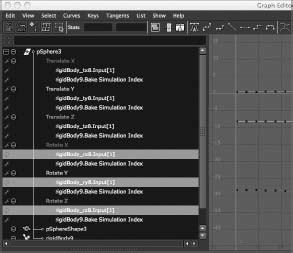
Figure 12.14 A simplified curve for the rotations of the eight ball

nParticle Dynamics
Like rigid body objects, particles are moved dynamically using collisions and fields. In short, a particle is a point in space that is given renderable properties—that is, it can render out. When particles are used en masse, they can create effects such as smoke, a swarm of insects, fireworks, and so on. nParticles are an implementation of particles through the Maya Nucleus solver, which provides better and easier simulations than traditional Maya particles.
Although particles (and nParticles) can be an advanced and involved aspect of Maya, it's important to have some exposure to them as you begin to learn Maya.
Much of what you learned about rigid body dynamics transfers to particles. However, it's important to think of particle animation as manipulating a larger system rather than as controlling every single particle in the simulation. Particles are most often used together in large numbers so that the entirety is rendered out to create an effect. You control fields and dynamic attributes to govern the motion of the system as a whole.
Emitting nParticles
A typical workflow for creating an nParticle effect in Maya breaks out into two parts: motion and rendering. First, you create and define the behavior of particles through emission. An emitter is a Maya object that creates the particles. After you create fields and adjust particle behavior within a dynamic simulation, much as you would do with rigid body motion, you give the particles renderable qualities to define how they look. This second aspect of the workflow defines how the particles come together to create the desired effect, such as steam. You'll make a locomotive pump steam later in this chapter.
To create an nParticle system, follow these steps:
Figure 12.15 Creation options for an nParticle emitter

- Make sure you're in the nDynamics menu set, choose nParticles Create nParticles, and select Cloud. Choose nParticles Create nParticles Create Emitter . The option box gives you various creation options for the nParticle emitter, as shown in Figure 12.15.
The default settings create an Omni emitter with a rate of 100 particles per second and a speed of 1.0. Click Create. A small round object (the emitter) appears at the origin.
- Click the Play button to play the scene. As with rigid body dynamics, you must also play back the scene using the Play Every Frame option. You can't scrub or reverse-play particles unless you create a cache file. You'll learn how to create a particle disk cache later in this chapter.
You'll notice a mass of round circles streaming out of the emitter in all directions (see Figure 12.16). These are the nParticles.
Emitter Attributes
You can control how particles are created and behave by changing the type of emitter and adjusting its attributes. Here are the most often used emitters:
Omni Emits particles in all directions.
Directional Emits a spray of particles in a specific direction, as shown in Figure 12.17.
Volume Emits particles from within a specified volume, as shown in Figure 12.18. The volume can be a cube, a sphere, a cylinder, a cone, or a torus. By default, the particles can leave the perimeter of the volume.
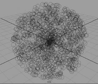
Figure 12.16 An Omni emitter emits a swarm of cloud particles in all directions.
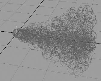
Figure 12.17 Cloud nParticles sprayed in a specific direction
After you create an emitter, its attributes govern how the particles are released into the scene. Every emitter has the following attributes to control the emission:
Rate Governs how many particles are emitted per second.
Speed Specifies how fast the particles move out from the emitter.
Speed Random Randomizes the speed of the particles as they're emitted, for a more natural look.
Min and Max Distance Emits particles within an offset distance from the emitter. You enter values for the Min and Max Distance settings. Figure 12.19 shows a Directional emitter with Min and Max Distance settings of 3.

Figure 12.18 Cloud nParticles emit from anywhere inside the emitter's volume.
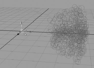
Figure 12.19 An emitter with Min and Max Distance settings of 3 emits Cloud nParticles three units from itself.
nParticle Attributes
After being created, or born, and set into motion by an emitter, nParticles rely on their own attributes and any fields or collisions in the scene to govern their motion, just like rigid body objects.
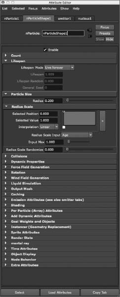
In Figure 12.20, the Attribute Editor shows a number of tabs for the selected particle object. Particle1 is the particle object node. This has the familiar Translate, Rotate, and Scale attributes, like most other object nodes. But the shape node, particleShape1, is where all the important attributes are for a particle, and it's displayed by default when you select a particle object. The third tab in the Attribute Editor is the emitter1 node that belongs to the particle's emitter. This makes it easier to toggle back and forth to adjust emitter and particle settings.
Figure 12.20 nParticle attributes
The Lifespan Attributes
When any particle is created, or born, you can give it a lifespan, which allows the particle to die when it reaches a certain point in time. As you'll see with the steam locomotive later in the chapter, a particle that has a lifespan can change over that lifespan. For example, a particle may start out as white and fade away at the end of its life. A lifespan also helps keep the total number of particles in a scene to a minimum, which helps the scene run more efficiently.
You use the Lifespan mode to select the type of lifespan for the nParticle:
Live Forever The particles in the scene can exist indefinitely.
Constant All particles die when their Lifespan value is reached. Lifespan is measured in seconds, so upon emission, a particle with a Lifespan of 1.0 will exist for 30 frames (in a scene set up at 30fps) before it disappears.
Random Range This type sets a lifespan in Constant mode but assigns a range value via the Lifespan Random attribute to allow some particles to live longer than others for a more natural effect.
LifespanPP Only This mode is used in conjunction with expressions that are programmed into the particle with Maya Embedded Language (MEL). Expressions are an advanced Maya concept and aren't used in this book.
The Shading Attributes
The Shading attributes determine how your particles look and how they will render. Two types of particle rendering are used in Maya: software and hardware. Hardware particles are typically rendered out separately from anything else in the scene and are then composited with the rest of the scene. Because of this compound workflow for hardware particles, this book will introduce you to a software particle type called Cloud. Cloud, like other software particles, can be rendered with the rest of a scene through the software renderer.
With your particles selected, open the Attribute Editor. In the Shading section, you'll find the Particle Render Type drop-down menu (see Figure 12.21).
The three render types listed with the (s/w) suffix are software-rendered particles. All the other types can be rendered only through the hardware renderer. Select your render type, and Maya adds the proper attributes you'll need for the render type you selected.
For example, if you select the Points render type from the menu, your particles change from circles on the screen to dots, as shown in Figure 12.22.
Several new attributes that control the look of the particles appear when you switch the Particle Render Type. Each Particle Render Type has its own set of render attributes. Set your nParticles back to the Cloud type. The Cloud particle type attributes are Threshold, Surface Shading, and Opacity. (See Figure 12.23.)
In the Shading heading, shown in Figure 12.24 for the Cloud nParticles, are controls for the Opacity Scale, Color, and Incandescence attributes. They control how the particles look when simulated and rendered. Notice how each of these controls is based on ramps.
nParticles are already set up to allow you to control the color, opacity, and incandescence during the life of the particle. For example, by default, the Color attribute is set up with a white to cyan ramp. This means that each of the particles will begin life white in color and will gradually turn cyan toward the end of its lifespan, or Age.
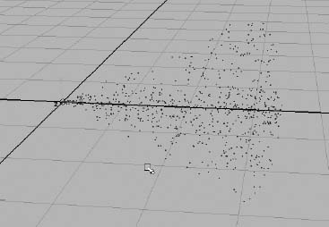
Figure 12.22 Dots on the screen represent Point particles.
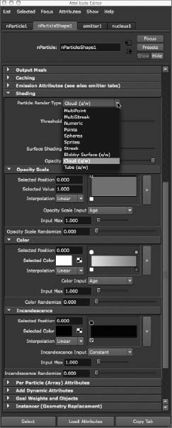
Figure 12.21 The Particle Render Type drop-down menu
Likewise, the Particle Size heading in the Attribute Editor contains a ramp for Radius Scale that works much the same way as the Color attribute just described. In this case, you use the Radius Scale ramp to increase or decrease the size of the particle along its Age.

Figure 12.23 Each Particle Render Type displays its own set of attributes.
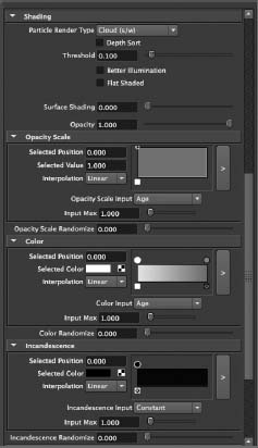
Figure 12.24 Controls for Opacity Scale, Color, and Incandescence attributes
nCaching Particles
It would be nice to turn particles into cash, but I can only show you how to turn your particles into a cache. You can cache the motion of your particles to memory or to disk to make playback and editing of your particle animation easier. To cache particles to your system's fast RAM memory, select the nParticle object you want to cache, and open the Attribute Editor. In the Caching section, under Memory Caching, select the Cache Data check box. Play back your scene, and the particles cache into your memory for faster playback. You can also scrub your timeline to see your particle animation. If you make changes to your animation, the scene won't reflect the changes until you delete the cache from memory by selecting the particle object and unchecking the Memory Cache check box in the Attribute Editor. The amount of information the memory cache can hold depends on your machine's system RAM.
Although memory caching is generally faster than disk caching, creating a disk cache lets you cache all the particles as they exist throughout their duration in your scene and ensures that the particles are rendered correctly, especially if you're rendering on multiple computers or across a network. You should create a particle disk cache before rendering.
If you make changes to your particle simulation but you don't see the changes reflected when you play back the scene, make sure you've turned off any memory or deleted any disk cache from previous versions of the simulation.
Creating an nCache on Disk
After you've created a particle scene, and you want to be able to scrub the timeline back and forth to see your particle motion and how it acts in the scene, you can create a particle nCache to disk. This lets you play back the entire scene as you like, without running the simulation from the start and by every frame.
To create an nCache, switch to the nDynamics menu, select the nParticle object, and choose nCache ![]() Create New Cache. Maya will run the simulation according to the timeline and save the position of all the particle systems in the scene to cache files in your current project's datacache folder. You can then play or even scrub your animation back and forth, and the particles will run properly.
Create New Cache. Maya will run the simulation according to the timeline and save the position of all the particle systems in the scene to cache files in your current project's datacache folder. You can then play or even scrub your animation back and forth, and the particles will run properly.
If you make any dynamics changes to the particles, such as emission rate or speed, you'll need to detach the cache file from the scene for the changes to take effect. Choose nCache ![]() Delete Cache. You can open the option box to select whether you wish to delete the cache files physically or merely detach them from the current nParticles.
Delete Cache. You can open the option box to select whether you wish to delete the cache files physically or merely detach them from the current nParticles.
Now that you understand the basics of particle dynamics, it's time to see for yourself how they work.
Animating a Particle Effect: Locomotive Steam
You'll create a spray of steam puffing out of the pump on the side of the locomotive that drives the wheels. You'll use the more detailed locomotive model from Chapter 8, “Introduction to Animation,” and Chapter 9, “More Animation!”
Emitting the nParticles
The first step is to create an emitter to spray from the steam pump and to set up the motion and behavior of the nParticles:
- In the nDynamics menu, choose nParticles Create nParticles. Cloud should still be checked in the Create nParticles menu. If it isn't, select Cloud, and then choose nParticles Create nParticles Create Emitter . Set Emitter Type to Directional, and click Create. Place the emitter at the end of the pump, as shown in Figure 12.25.
Figure 12.25 Place the emitter at the end of the pump.

- To set up the emission in the proper direction, adjust the attributes of the emitter. In the Distance/Direction Attributes section, set Direction Y to 0, Direction X to 0, and Direction Z to 1. This emits the particles straight out of the pump over the first large wheel and toward the back of the engine.
The Direction attributes are relative. Entering a value of 1 for Direction X and a value of 2 for Direction Y makes the particles spray at twice the height (Y) of their lateral distance (X).
- Play back your scene. The Cloud nParticles emit in a straight line from the engine, as shown in Figure 12.26.
You can load the file Locomotive_Steam_v1.ma from the Locomotive project on the web page to check your work.
- To change the particle emission to more of a spray, adjust the Spread attribute for the emitter. Click the emitter1 tab in the particle's Attribute Editor (or select the emitter to focus the Attribute Editor on it instead), and change Spread from 0 to 0.30. Figure 12.27 shows the new cloud spray.

Figure 12.26 Cloud nParticles emit in a straight line from the pump.
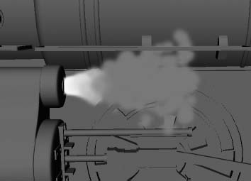
Figure 12.27 The emitter's Spread attribute widens the spray of particles.
The Spread attribute sets the cone angle for a directional emission. A value of 0 results in a thin line of particles. A value of 1 emits particles in a 180-degree arc.
- The emission is rather slow for hot steam being pumped out as the locomotive drives the wheels, so change the Speed setting for the emitter from 1 to 2.0, and change Speed Random from 0 to 1. Doing so creates a random speed range between 1 and 3 for each particle. These two attributes are found in the emitter's Attribute Editor in the Basic Emission Speed Attributes section.
- So that all the steam doesn't emit from the same point, keep the emitter's Min Distance at 0 but set its Max Distance to 0.3. This creates a range of offset between 0 and 0.3 units for the particle to emit from, as shown in Figure 12.28.
Figure 12.28 A range of offset between 0 and 0.3 units creates a more believable emission.

Setting nParticle Attributes
It's always good to get the particles moving as closely to what you need as possible before you tend to their look. Now that you have the particles emitting properly from the steam pump, you'll adjust the nParticle attributes. Start by setting a lifespan for them, and then add rendering attributes:
Figure 12.29 The initial radius settings for the steam nParticles

- Select the nParticle object, and open the Attribute Editor. In the Lifespan section, set Lifespan Mode to Random Range. Set Lifespan to 2 and Lifespan Random to 1. This creates a range of 1 to 3 for each particle's lifespan. (This is based on a lifespan of 3, plus or minus a random value from 0 to 1.)
- You can control the radius of the particles as they're emitted from the pump. Under the Particle Size heading in the Attribute Editor, set a Radius attribute of 0.50. Set the Radius Scale Randomize attribute to 0.25. This allows you to have particles that emit with a radius range between 0.25 and 0.75. Figure 12.29 shows the attributes.
- If you play back the simulation, you see the particles are quite large initially. Because steam expands as it travels, you need to adjust the size (radius) of your nParticles to make them smaller at birth; they will grow larger over their lifespan and produce a good look for your steam.
- In the Radius Scale heading in the Attribute Editor, click the arrow to the right of the ramp to open a larger view of the ramp, as shown in Figure 12.30.
Figure 12.30 Open the Radius Scale ramp.
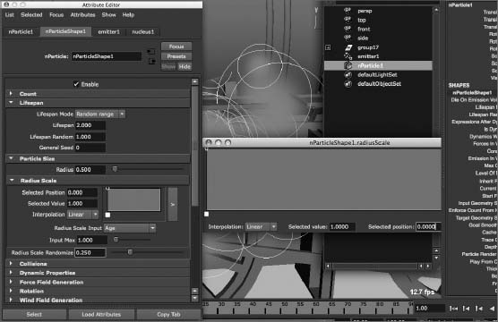
- Click and drag the ramp's first and only handle (an open circle at the upper-left corner of the Ramp window) down to a value of about 0.25, as shown in Figure 12.31. The particles get smaller as you adjust the ramp value.
Figure 12.31 Decrease the radius of the nParticles using the Radius Scale ramp.
- To allow the particles to grow in size, add a second handle to the scale curve by clicking anywhere on that line, and drag to a value of 1.0 and the position shown in Figure 12.32. The particles toward the end of the spray get larger.
Figure 12.32 Adjust the Radius Scale ramp to grow the particles.

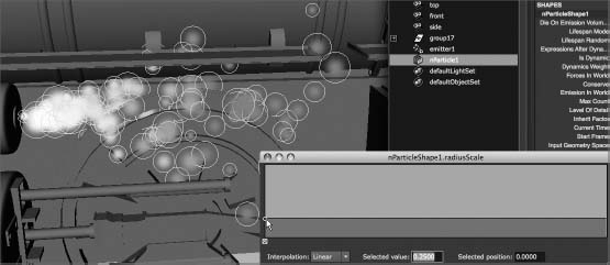
- You can set up collisions so the nParticle steam doesn't travel right through the mesh of the locomotive. Select the meshes shown in Figure 12.33, and choose nMesh Create Passive Collider.
- In the Outliner, select the three nRigid nodes that were just created, and set the Friction attribute in the Channel Box to 0.0 from the default of 0.10. Play back your scene, and your particles now collide with the surface of the locomotive. (See Figure 12.34.)
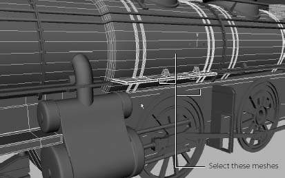
Figure 12.33 Select the meshes with which the nParticles will collide.

Figure 12.34 The particles now react very nicely against the side of the locomotive.
If you want to check your work, download the file locomotive_steam_v2.ma from the Locomotive project on the web page.
Setting Rendering Attributes
After you define the nParticle movement to your liking, you can create the proper look for the nParticles. This means setting and adjusting their rendering parameters. Because Maya has several types of particles, the particles are set up according to their type; the following workflow applies only to the Cloud particle type:
- Select the nParticle object, and open the Attribute Editor. Expand the Shading heading, and look at the Color ramp. By default, the particles go from white to light blue in color. Click the cyan color's circle handle on top of the ramp. The Selected Color attribute next to the ramp shows the cyan color. Click in the swatch to open the Color Chooser, and change the color to a very light gray.
- Click the arrow bar to the right of the Opacity Scale ramp to open a larger ramp view. Grab the first handle in the upper-left corner, and drag it down to a value of 0.12.
- The steam needs to be less opaque at its birth, grow more opaque toward the middle of its life, and fade completely away at the end of the particle's life. Click to create new handles to create a curve for the ramp, as shown in Figure 12.35. The values for the five ramp handles shown from left to right are 0.12, 0.30, 0.20, 0.08, and 0.
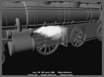
- In the Render Settings window, set Image Size to 640 × 480. In the Maya Software tab, set Quality to Intermediate Quality. Run the animation, and stop it when some steam has been emitted. Render a frame. It should look like Figure 12.36. The steam doesn't travel far enough along the engine; it disappears too soon.

Figure 12.35 Creating an Opacity ramp for the steam

Figure 12.36 The steam seems too short and small.
With the steam nParticles selected, open the Attribute Editor and, in the Radius Scale, change the first handle's value from 0.25 to 0.35 to make the steam particles a bit larger. Below the Opacity Scale ramp is the Input Max slider; set that value to 1.6.
- Select the emitter1 tab, and change the Spread value for the emitter to 0.2. Change Rate (Particles/Sec) to 200 and Speed to 3.0. Play back the simulation, and render a frame to compare to Figure 12.37.
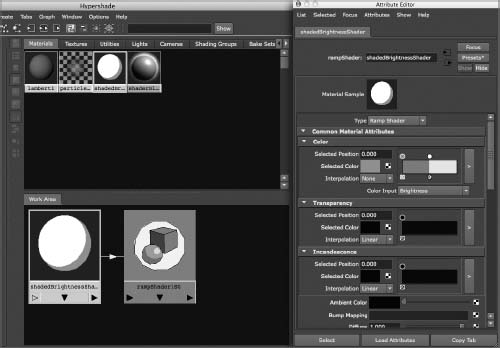
- The Color ramp in the nParticle's Attribute Editor controls the color of the steam, and a shader is assigned to the particles. Select the steam nParticle object, and open the Hypershade window. In the Hypershade, click the Graph materials on the selected object's icon (
 ), as shown in Figure 12.38.
 - In the Hypershade, select the npCloudVolume shader, and open the Attribute Editor. Notice that the Common Material Attributes section's attributes all have connections. The ramp controls in the nParticle Attribute Editor are controlling the attributes in this Particle Cloud shader.
- Under the Transparency heading in the Attribute Editor for the shader, set Density to 0.35. Try a render; the steam should look better. (See Figure 12.39.)
Figure 12.37 A better emission, but a bit too solid
Batch-render a 200-frame sequence of the scene at a lower resolution, such as 320 × 240, to see how the particles look as they animate. (Check the frames with FCheck. Refer to Chapter 11, “Maya Rendering,” for more on FCheck.)
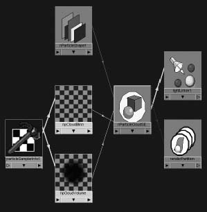
Figure 12.38 The shaders assigned to the Cloud nParticle
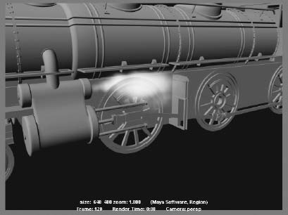
Figure 12.39 The steam is less flat and solid.
Download the file locomotive_steam_v3.ma from the Locomotive project on the web page to check your work.
Experiment with the steam by animating the Rate attribute of the emitter to make the steam pump out in time with the wheel arm. Also, try animating the Speed values and playing with different values in the Radius and Opacity ramps. The steam you'll get in this tutorial looks pretty good, but it isn't as lifelike as it could be. Particle animators are always learning new tricks and expanding their skills, and that comes from always trying new things and retrying the same effects with different methods.
When you feel comfortable with the steam exercise, try using the Cloud nParticle to create steam for a mug of coffee. That steam moves much more slowly and is less defined than the blowing steam of the locomotive, and it should pose a new challenge. Also try your hand at creating a smoke trail for a rocket ship or a wafting stream of cigarette smoke, or even the billowing smoke coming from the engine's chimney.
Cloud nParticles are the perfect particle type with which to begin. As you feel more comfortable animating with clouds, experiment with the other render types. The more you experiment with all the types of nParticles, the easier they will be to harness.
Introduction to Paint Effects
One of the tools in Maya's effects arsenal is called Paint Effects. Using Paint Effects, you can create a field of grass rippling in the wind, a head of hair or feathers, or even a colorful aurora in the sky. Paint Effects is a rendering effect found under the Rendering menu. It has incredible dynamic properties that can make leaves rustle in the wind or trees sway in a storm. Paint Effects uses its own dynamics calculations to create natural motion.
It's one of Maya's most powerful tools, with features that go far beyond the scope of this introductory book. Here you'll learn how to create a Paint Effects scene and how to access all the preset brushes to create your own effects.
Paint Effects uses brushes to paint effects into your 3D scene. The brushes create strokes on a surface or in the Maya modeling views that produce tubes, which render out through Maya's software renderer. These Paint Effects tubes have dynamic properties, which means they can move according to their own forces. Therefore, you can easily create a field of blowing grass.
Try This Create a field of blowing grass and flowers; it will take you all of five minutes.
- Start with a new scene file. Maximize the perspective view. (Press the spacebar with the Perspective window active.)
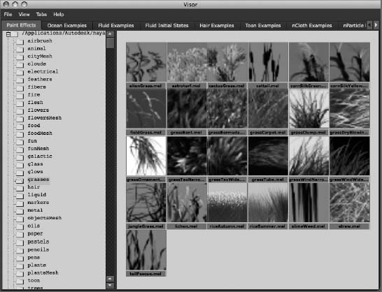
- Switch to the Rendering menu set (press F6). Choose Paint Effects Get Brush to open the Visor window. The Visor window displays all the preset Paint Effects brushes that automatically create certain effects. Select the Grasses folder in the Visor's left panel to display the grass brushes available (see Figure 12.40). You can navigate the Visor window as you would navigate any other Maya window, using the Alt key and the mouse buttons.
- Click the grassWindWide.mel brush to activate the Paint Effects tool and set it to this grass brush. Your cursor changes to a Pencil icon.
Figure 12.40 The preset grass brushes in the Visor window
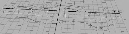
- In the Perspective window, click and drag two lines across the grid, as shown in Figure 12.41, to create two Paint Effects strokes of blowing grass. If you can't see the grass in your view panel, increase Global Scale in the Paint Effects Brush Settings in either the Attribute Editor or the Channel Box to see the grass being drawn onto the screen.
Figure 12.41 Click and drag two lines across the grid.

- To change your brush so you can add some flowers between the grass, choose Paint Effects Get Brush, and select the flowers folder. Select the dandelion_Yellow.mel brush. Your Paint Effects tool is now set to paint yellow flowers.
- Click and drag a new stroke between the strokes of grass, as shown in Figure 12.42.
Figure 12.42 Add new strokes to add flowers to the grass.
- Position your camera, and render a frame. Make sure you're using Maya Software and not mental ray to render through the Render Settings window and that you use a large enough resolution, such as 640 × 480, so that you can see the details. Render out a 120-frame sequence to see how the grass animates in the wind. Figure 12.43 shows a scene filled with grass strokes as well as a number of different flowers.
After you create a Paint Effects stroke, you can edit the look and movement of the effect through the Attribute Editor. You'll notice, however, that there are a large number of attributes to edit with Paint Effects. The next section introduces the attributes that are most useful to the beginning Maya user.
Figure 12.43 Paint Effects can add realistic flowers and grass to any scene.

Paint Effects Attributes
It's best to create a single stroke of Paint Effects in a blank scene and experiment with adjusting the various attributes to see how they affect the strokes. Select the stroke, and open the Attribute Editor. Switch to the stroke's tab to access the attributes. For example, for an African Lily Paint Effects stroke, the Attribute Editor tab is called africanLily1.
Each Paint Effects stroke produces tubes that render to create the desired effect. Each tube (you can think of a tube as a stalk) can grow to have branches, twigs, leaves, flowers, and buds. Each section of a tube has its own controls to give you the greatest flexibility in creating your effect. As you experiment with Paint Effects, you'll begin to understand how each attribute contributes to the final look of the effect.
Here is a summary of some Paint Effects attributes:
Brush Profile Gives you control over how the tubes are generated from the stroke; this is done with the Brush Width attribute. This attribute makes tubes emit from a wider breadth from the stroke to cover more of an area.
Shading and Tube Shading Gives you access to the color controls for the tubes on a stroke.
Color1 and Color2 From bottom to top, graduates from Color1 to Color 2 along the stalk only. The leaves and branches have their own color attributes, which you can display by choosing Tubes ![]() Growth.
Growth.
Incandescence1 and 2 Adds a gradient self-illumination to the tubes.
Transparency1 and 2 Adds a gradient transparency to each tube.
Hue/Sat/Value Rand Add some randomness to the color of the tubes.
In the Tubes section, you'll find all the attributes to control the growth of the Paint Effects effect. In the Creation subsection, you can access the following:
Tubes Per Step Controls the number of tubes along the stroke. For example, this setting increases or decreases the number of flowers for the africanLily1 stroke.
Length Min/Max Controls how tall the tubes are grown to make taller flowers or grass (or other effects).
Tube Width1 and Width2 Controls the width of the tubes (the stalks of the flowers).
In the Growth subsection, you can access controls for branches, twigs, leaves, flowers, and buds for the Paint Effects strokes. Each attribute in these sections controls the number, size, and shape of those elements. Although not all Paint Effects strokes create flowers, all strokes contain these headings.
The Behavior subsection contains the controls for the dynamic forces affecting the tubes in a Paint Effects stroke. Adjust these attributes if you want your flowers to blow more in the wind.
Paint Effects are rendered as a postprocess, which means they won't render in reflections or refractions as is and they will not render in mental ray without conversion to polygons. They're processed and rendered after every other object in the scene is rendered out in Maya Software rendering only.
To render Paint Effects in mental ray, you can convert Paint Effects to polygonal surfaces. They will then render in the scene along with any other objects so that they may take part in reflections and refractions. To convert a Paint Effects stroke to polygons, select the stroke and choose Modify ![]() Convert
Convert ![]() Paint Effects To Polygons. The polygon Paint Effects tubes can still be edited by most of the Paint Effects attributes mentioned so far; however, some, such as color, don't affect the poly tubes. Instead, the color information is converted into a shader that is assigned to the polygons. It's best to finalize your Paint Effects strokes before converting to polygons, to avoid any confusion.
Paint Effects To Polygons. The polygon Paint Effects tubes can still be edited by most of the Paint Effects attributes mentioned so far; however, some, such as color, don't affect the poly tubes. Instead, the color information is converted into a shader that is assigned to the polygons. It's best to finalize your Paint Effects strokes before converting to polygons, to avoid any confusion.
Paint Effects is a strong Maya tool and you can use it to create complex effects such as a field of blowing flowers. A large number of controls to create a variety of effects come with that complexity. Fortunately, Maya comes with a generous sampling of preset brushes. Experiment with a few brushes and their attributes to see what kinds of effects and strange plants you can create.
Toon Shading
Paint Effects has been developed into a toon-shading system to make your animations render more like traditional cartoons. Using Paint Effects, Maya renders outlines for the objects in your scene, and using a Toon shader, Maya renders the objects in the scene with a flat cartoon-color look. Next, we'll take a quick look at how to apply toon shading to the wagon scene to make it render like a cartoon.
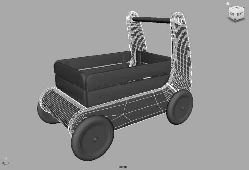
Try This Set your project to the RedWagon project, and open the RedWagonModel_v08.ma scene file from the Scenes folder.
- You'll see the wagon in a ¾ view in the persp view panel. Select all the parts of the body of the wagon without the railings, as shown in Figure 12.44.
Figure 12.44 Select the main body of the wagon, without the wheels or the rails.
- Switch to the Rendering menu set, and select Toon Assign Fill Shader Shaded Brightness Two Tone. The Attribute Editor opens, focused on a Ramp shader as shown in Figure 12.45.
Figure 12.45 A Ramp shader is added to the scene and applied to the wagon's body.
- Under the Color heading, set the color of the gray part of the ramp to a dark red, and set the white part of the ramp to a bright red. Your wagon should turn red in the persp view panel if you're in Shaded or Texture view. Render a frame, and you should see the wagon in only two tones of red but with gray railings and wheels (shown in grayscale in Figure 12.46).
- Select the rail objects, and select Toon Assign Fill Shader Shaded Brightness Two Tone to create another Toon shader. Set the colors to a dark tan and a bright tan color in the Color ramp.
- Select the handlebar and all four wheels and create another two-tone fill shader with a gray and white Color ramp (which is the default).
- The frame, railings, and wheels now have a Toon shader as well. Notice the wheels in Figure 12.47 and how cool they look when toon shaded. Of course, adjust any of the colors to your liking.
- Now for the toon outlines. Select all the parts of the wagon, and select Toon Assign Outline Add New Toon Outline. A black outline appears around the outside of the wagon's parts, and a new node called pfxToon1 appears in the Outliner or Hypergraph. The outlining is accomplished with Paint Effects.
- Before you render a frame, set the background to white to make the black toon outlines pop. To do so, select the persp camera and open the Attribute Editor. Under the Environment heading, set Background Color to white.
- Open the Render Settings window, and set the renderer to Maya Software. Render a frame, and compare to Figure 12.48. The outlines are too thick!
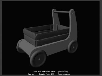
Figure 12.46 The wagon now has a toon-shaded body. The front side of the wagon is a darker red than the front, due to the lighting in the scene.

Figure 12.47 The wagon has Toon shaders for the fill color applied.
- Select the pfxToon1 node in the Outliner, and open the Attribute Editor window. Click the pfxToonShape1 tab to open the attributes for the outlines. Set the Line Width attribute to 0.03, and render a frame. Compare to Figure 12.49.
You can adjust the colors and the ramps of the Fill shader to suit your tastes, and you can try out the other Fill shader types, such as a three-tone shader to get a bit more detail in the coloring of the wagon. Adjust the toon outline thickness as you like, and have some fun playing with the toon outline's attributes to see how they affect the toon rendering of the wagon. This should be a quick primer to get you into toon shading. The rest, as always, is up to you. With some playing and experimenting, and you'll be rendering some pretty nifty cartoon scenes in no time.
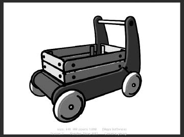
Figure 12.48 The black outlines are applied, but they're too thick.
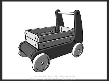
Figure 12.49 The cartoon wagon!
Customizing Maya
One of Maya's most endearing features is its almost infinite customizability. Everyone has different tastes, and everyone works in their own way. Simply put, for everything there is to do in Maya, you have several ways of doing it; there are at least a couple of different ways to access Maya's tools, features, and functions as well.
This flexibility may be confusing at first, but you'll discover that in the long run it's very advantageous. The ability to customize enables the greatest flexibility in individual workflow.
It's best to use Maya at its defaults as you first learn. However, when you feel comfortable enough with your progress, you can use this section to change some of the interface elements in Maya to better suit how you like to work.
Figure 12.50 The Settings/Preferences menu
User Preferences
All the customization features are found under Window ![]() Settings/Preferences, which displays the window shown in Figure 12.50.
Settings/Preferences, which displays the window shown in Figure 12.50.
The Preferences window (see Figure 12.51) lets you make changes to the look of the program as well as to toolset defaults by selecting from the categories listed in the left pane of the window.
The Preferences window is separated into categories that define different aspects of the program. Interface and Display deal with options to change the look of the program. Interface affects the main user interface, whereas Display affects how objects are displayed in the workspace.
Figure 12.51 The Preferences window
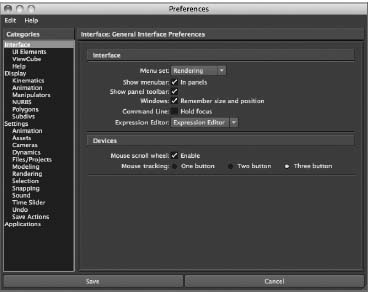
The Settings category lets you change the default values of several tools and their general operation. An essential aspect of this category is Working Units: these options set the working parameters of your scene (in particular, the Time setting).
By adjusting the Time setting, you tell Maya your frame rate of animation. If you're working in film, you use a frame rate of 24 frames per second (fps). If you're working in NTSC video (the standard video/television format in the Americas), you use the frame rate of 30 fps.
The Applications category lets you specify which applications you want Maya to start automatically when a function is called. For example, while looking at the Attribute Editor for a texture image, you can click a single button to open that image in your favorite image editor, which you specify here.
Under the Settings section, click the Undo header and set the Undo Queue to Infinite. Doing so allows you to undo as many actions as have occurred since you loaded the file. This feature is unbelievably handy, especially when you're first learning Maya.
Shelves
Under the Shelf Editor command (Window ![]() Settings/Preferences
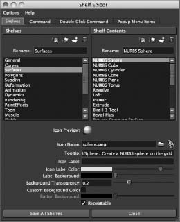
Settings/Preferences ![]() Shelf Editor) lurks a window that manages your shelves (see Figure 12.52). You can create or delete shelves, or manage the items on the Shelf with this function. This is handy when you create your own workflow for a project. Simply click the Shelves tab to display the icons on that Shelf in the Shelf Editor window. Click in the Shelf Contents section to edit the icons and where they reside on that selected Shelf. Clicking the Command tab gives you access to the MEL command for that icon when it is single-clicked in the Shelf. Click the Double Click Command tab for the MEL command for the icon when it is double-clicked in the Shelf.
Shelf Editor) lurks a window that manages your shelves (see Figure 12.52). You can create or delete shelves, or manage the items on the Shelf with this function. This is handy when you create your own workflow for a project. Simply click the Shelves tab to display the icons on that Shelf in the Shelf Editor window. Click in the Shelf Contents section to edit the icons and where they reside on that selected Shelf. Clicking the Command tab gives you access to the MEL command for that icon when it is single-clicked in the Shelf. Click the Double Click Command tab for the MEL command for the icon when it is double-clicked in the Shelf.
You can also edit Shelf icons from within the UI without the Shelf Editor window. To add a menu command to the current Shelf, hold down Ctrl+Alt+Shift, and click the function or command directly from its menu. Items from the Tool Box, pull-down menus, or the Script Editor may be added to any Shelf:
- To add an item from the Tool Box, MMB+drag its icon from the Tool Box into the appropriate Shelf.
- To add an item from a menu to the current Shelf, hold down the Ctrl+Alt+Shift keys while selecting the item from the menu.
- To add an item (a MEL command) from the Script Editor, highlight the text of the MEL command in the Script Editor, and MMB+drag it onto the Shelf. A MEL icon will be created that will run the command when you click it.
- To remove an item from a Shelf, MMB+drag its icon to the Garbage Can icon at the end of the Shelf, or use Window Settings/Preferences Shelf Editor.
Hotkeys
Hotkeys are keyboard shortcuts that can access almost any Maya tool or command. You've already encountered a few in your exploration of the interface and in the Solar System exercise in Chapter 2. What fun! You can create even more hotkeys, as well as reassign existing hotkeys, through the Hotkey Editor, shown in Figure 12.53 (Window ![]() Settings/Preferences
Settings/Preferences ![]() Hotkey Editor).
Hotkey Editor).
Through this monolith of a window, you can set a key combination to be used as a shortcut to virtually any command in Maya. This is the last customization you want to touch. Because so many tools have hotkeys assigned by default, it's important to get to know them first before you start changing things to suit how you work.
Every menu command is represented by menu categories on the left; the right side allows you to view the current hotkey or assign a new hotkey to the selected command. Ctrl and Alt key combinations may be used with any letter keys on the keyboard. Keep in mind that Maya is case sensitive, meaning that it differentiates between uppercase and lowercase letters. For example, one of my personal hotkeys is Ctrl+H to hide the selected object from view; Shift+Ctrl+H unhides it. (I'm sharing.)
Figure 12.53 The Hotkey Editor
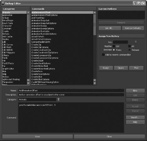
The lower section of this window displays the MEL command that the menu command invokes. It also allows you to type in your own MEL commands, name them as new commands, categorize them with the other commands, and assign hotkeys to them.
The important thing to focus on right now is discovering how to use the tools to accomplish the tasks you need to perform and establishing a basic workflow. Toward that end, I strongly suggest learning Maya in its default configuration and only using the menu structure and default shelves to access all your commands at first, with the exception of the most basic hotkeys.
Color Settings
You can set the colors for almost any part of the interface to your liking through the Colors window shown in Figure 12.54 (Window ![]() Settings/Preferences
Settings/Preferences ![]() Color Settings).
Color Settings).
The window is separated into different aspects of the Maya interface by headings. The 3D Views heading lets you change the color of all the panels' backgrounds. For example, color settings give you a chance to set the interface to complement your office's décor as well as make certain items easier to read.
Customizing Maya is important. However—and this can't be stressed enough—it's important to get your bearings with default Maya settings before you venture out and change hotkeys and such. When you're ready, this section of this chapter will still be here for your reference.
Summary
In this chapter, you learned how to create dynamic objects and create simulations. Beginning with rigid body dynamics, you created a set of pool balls that you animated in the simulation to knock into each other. Then, you learned how to bake that simulation into animation curves for fine-tuning. Next, you learned about particle effects by creating a steam effect for the locomotive animation using nParticles. Finally, you learned a little about Maya's Paint Effects tool and how you can easily use it to create various effects such as grass and flowers. Then you used toon shading on the wagon and finally glossed over some of the customization options available in the Maya UI.
To further your learning, try creating a scene on a grassy hillside with train tracks running through. Animate the locomotive, steam and all, driving through the scene and blowing the grass as it passes. You can also create a train whistle and a steam effect when the whistle blows, and you can create various other trails of smoke and steam as the locomotive drives through.
The best way to be exposed to Maya dynamics is simply to experiment once you're familiar with the general workflow in Maya. You'll find that the workflow in dynamics is more iterative than other Maya workflows, because you're required to experiment frequently with different values to see how they affect the final simulation. With time, you'll develop a strong intuition, and you'll accomplish more complex simulations faster and with greater effect.
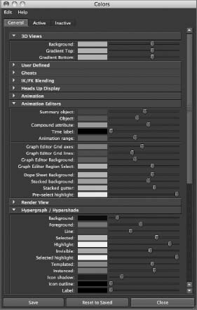
Figure 12.54 Changing the interface colors is simple.
Where Do You Go from Here?
It's so hard to say goodbye! But this is really a “hello” to learning more about animation and 3D!
Please explore other resources and tutorials to expand your working knowledge of Maya. Several websites contain numerous tips, tricks, and tutorials for all aspects of Maya, including the author's columns in HDRI3d magazine (www.hdri3d.com) and my occasional ramblings online at http://kooshspot.blogspot.com/ and on Facebook at facebook.com/IntroMaya.
Of course, www.autodesk.com/maya has a wide range of learning tools. Be sure to check out the sidebar “Suggested Reading” in the absolutely fabulous Chapter 1, “Introduction to Computer Graphics and 3D.” Now that you've gained your all-important first exposure, you'll be better equipped to forge ahead confidently.
The most important thing you should have learned from this book is that proficiency and competence with Maya come with practice, but even more so from your own artistic exploration. Treat this text and your experience with its information as a formal introduction to a new language and way of working for yourself; doing so is imperative. The rest of it—the gorgeous still frames and eloquent animations—come with furthering your study of your own art, working diligently to achieve your vision, and having fun along the way. Enjoy, and good luck.