
Logical Organization
A cache’s logical organization embodies two primary concepts:
1. Physical parameters that determine how the cache is addressed, how it is searched, and what it can store
2. Whether the cache is responsible for performing the various management heuristics on the client’s behalf, or whether the client (e.g., a software application using the cache) is responsible
The logical organization of a cache influences how the data is stored in the cache and how it is retrieved from the cache. Deciding what to store is a different issue and will be covered in following chapters, as will the topic of maintaining the data’s consistency. However, and this is an extremely important point, though the determination of what to store is made by a set of heuristics executed at design time and/or run time, the logical organization of the cache also indirectly determines what to cache. While the content-management heuristics make explicit choices of what to cache, the logical organization makes implicit choices; to wit, the determination of what to store can be, and often is, overridden by the cache’s logical organization, because the logical organization determines how and where data is stored in the cache. If the organization is incapable of storing two particular data items simultaneously, then, regardless of how important those two data items may be, one of them must remain uncached while the other is in the cache.
Thus, a cache’s logical organization is extremely important, and over the years many exhaustive research studies have been performed to choose the “best” organization for a particular cache, given a particular technology and a particular set of benchmarks. In general, a cache organization that places no restrictions on what can be stored and where it can be placed would be best (i.e., a fully associative cache), but this is a potentially expensive design choice.
2.1 Logical Organization: A Taxonomy
The previous chapter introduced transparent caches and scratch-pad memories. Because they are used differently, transparent caches and scratch-pad memories have different implementations and, more importantly, different ramifications. Because they lie at opposite ends of a continuum of design architectures, they define a taxonomy, a range of hybrid cache architectures that lie between them based on their most evident characteristics, including their methods of addressing and content management.
• Addressing Scheme: Transparent caches use the naming scheme of the backing store: a program references the cache implicitly and does not even need to know that the cache exists. The scratch-pad, by contrast, uses a separate namespace from the backing store: a program must reference the scratch-pad explicitly. Note that, because they could potentially hold anything in the space, transparent caches require keys or tags to indicate what data is currently cached. Scratch-pad memories require no tags.
• Management Schemes: The contents of traditional caches are managed in a manner that is transparent to the application software: if a data item is touched by the application, it is brought into the cache, and the consistency of the cached data is ensured by the cache. Scratch-pad random-access memories (RAMs) require explicit management: nothing is brought into the scratchpad unless it is done so intentionally by the application software through an explicit load and store, and hardware makes no attempt to keep the cached version consistent with main memory.
These two parameters define a taxonomy of four1 basic cache types, shown in Table 2.1:
TABLE 2.1
| Cache Type | Addressing Scheme | Management Scheme |
| Transparent cache | Transparent | Implicit (by cache) |
| Software-managed cache | Transparent | Explicit (by application) |
| Self-managed scratch-pad | Non-transparent | Implicit (by cache) |
| Scratch-pad memory | Non-transparent | Explicit (by application) |
• Transparent Cache: An application can be totally unaware of a transparent cache’s existence. Examples include nearly all general-purpose processor caches.
• Scratch-Pad Memory: When using a scratch-pad memory, the application is in control of everything. Nothing is stored in the cache unless the application puts it there, and the memory uses a separate namespace disjoint from the backing store. Examples include the tagless SRAMs used in DSPs and microcontrollers.
• Software-Managed Cache: In a software-managed cache, the application software controls the cache’s contents, but the cache’s addressing scheme is transparent—the cache uses the same namespace as the backing store, and thus, the cache can automatically keep its contents consistent with the backing store. Examples include the software-controlled caches in the VMP multiprocessor [Cheriton et al. 1986], in which a software handler is invoked on cache misses and other events that require cache-coherence actions.
• Self-Managed Scratch-Pad: In a self-managed scratch-pad, the cache contents are managed by the cache itself (e.g., in a demand-fetch manner or some other heuristic), and the cache’s storage uses a separate namespace from the backing store, addressed explicitly by application software. Examples include implementations of distributed memory, especially those with migrating objects (e.g., Emerald [Jul et al. 1988]).
Figure 2.1 shows the four different types of cache organization. Each has its own implementation and design issues, and each expects different things of the software running on the machine. For purposes of discussion in this chapter, the primary classification will be the addressing mechanism (transparent or non-transparent); within this classification, the cache’s contents can either be managed explicitly by the client or by the cache itself.
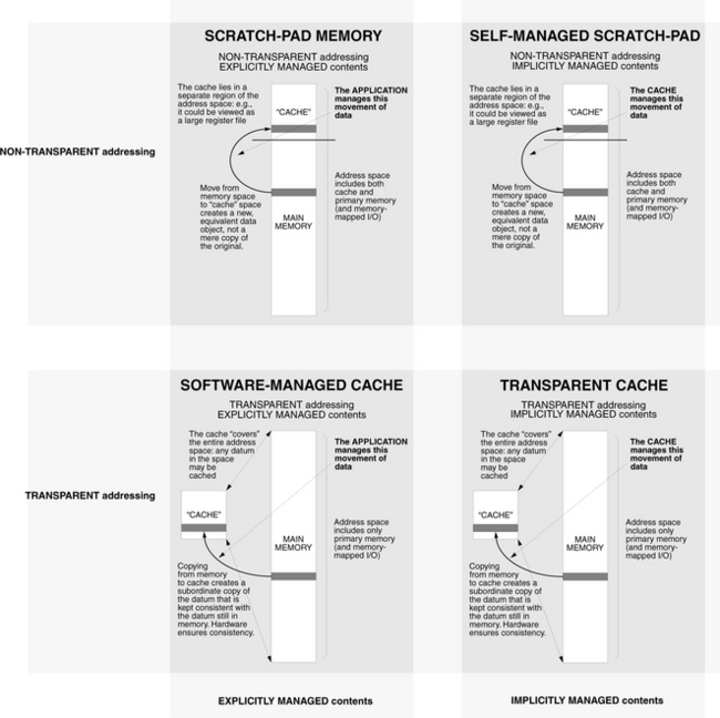
FIGURE 2.1 Examples of several different cache organizations. Though this illustrates “cache” in the context of solid-state memories (e.g., SRAM cache and DRAM main memory), the concepts are applicable to all manners of storage technologies, including SRAM, DRAM, disk, and even tertiary (backup) storage such as optical disk and magnetic tape.
2.2 Transparently Addressed Caches
A transparently addressed cache uses the same namespace as the backing store; that is, a cache lookup for the desired data object uses the same object name one would use when accessing the backing store. For example, if the backing store is the disk drive, then the disk block number would be used to search (or “probe”) the cache. If the backing store is main memory, then the physical memory address would be used to search the cache. If the backing store is a magneto-optical or tape jukebox, then its associated identifier would be used. The mechanism extends to software caches as well. For example, if the backing store is the operating system’s file system, then the file name would be used to search the cache. If the backing store is the world-wide web, then the URL would be used, and so on. The point is that the client (e.g., application software or even an operating system) need not know anything about the cache’s organization or operation to benefit from it. The client simply makes a request to the backing store, and the cache is searched for the requested object implicitly.
Because the cache must be searched (a consequence of the fact that it is addressed transparently and not explicitly), there must be a way to determine the cache’s contents, and thus, an implicitly addressed cache must have keys or tags, most likely taken from the backing store’s namespace as object identifiers. For instance, a software cache could be implemented as a binary search tree, a solid-state cache could be implemented with a tag store that matches the organization of the data store, or a DRAM-based cache fronting a disk drive could have a CAM lookup preceding data access to find the correct physical address [Braunstein et al. 1989]. Note that this is precisely what the TLB does.
Because the cost of searching can be high (consider, for example, a large cache in which every single key or tag is checked for every single lookup), different logical organizations have been developed that try to accomplish simultaneously two goals:
Note that these goals tend to pull a cache design in opposite directions. For instance, an easy way to satisfy Goal 1 is to assign a particular data object a single space in the cache, kind of like assigning the parking spaces outside a company’s offices. The problem with this is that, unless the cache is extremely large, one can quickly run out of spaces to assign, in which case the cache might have to start throwing out useful data (as an analogy, a company might have to reassign to a new employee a parking spot belonging to the company’s CEO).
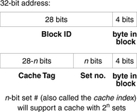
Basic organization for implicitly addressed caches has already been discussed briefly in Chapter 1. The main point is that a transparent cache typically divides its storage into equivalence classes, or sets, and assigns blocks to sets based on the block Id. The single, unique set to which a particular chunk of data belongs is typically determined by a subset of bits taken from its block ID, as shown in Figure 2.2. Once the set is determined, the block may be placed anywhere within that set. Because a block’s ID, taken from its location in the memory space, does not change over the course of its lifetime (exceptions including virtually indexed caches), a block will not typically migrate between cache sets. Therefore, one can view these sets as having an exclusive relationship with each other, and so any heuristic that chooses a partitioning of data between exclusive storage units would be just as appropriate as the simple bit-vector method shown in Figure 2.2.
A cache can comprise one or more sets; each set can comprise one or more storage slots. This gives rise to the following organizations for solid-state designs.
• Direct-Mapped Organization: Figure 2.3 illustrates a read operation in a direct-mapped cache organization. In this organization, a given datum can only reside in one entry of the cache, usually determined by a subset of the datum’s address bits. Though the most common index is the low-order bits of the tag field, other indexing schemes exist that use a different set of bits or hash the address to compute an index value bearing no obvious correspondence to the original address. Whereas in the associative scheme there are n tag matches, where n is the number of cache lines, in this scheme there is only one tag match because the requested datum can only be found at one location: it is either there or nowhere in the cache.

FIGURE 2.3 Block diagram for a direct-mapped cache. Note that data read-out is controlled by tag comparison with the TLB output as well as the block-valid bit (part of the tag or metadata entry) and the page permissions (part of the TLB entry). Data is not read from the cache if the valid bit is not set or if the permissions indicate an invalid access (e.g., writing a read-only block). Note also that the cache size is equal to the virtual memory page size (the cache index does not use bits from the VPN).
• Fully Associative Organization: Figure 2.4 demonstrates a fully associative lookup. In a fully associative organization, the cache is truly a small hardware database. A datum can be placed anywhere in the cache; the tag field identifies the data contents. A search checks the tag of every datum stored in the cache. If any one of the tags matches the tag of the requested address, it is a cache hit: the cache contains the requested data.
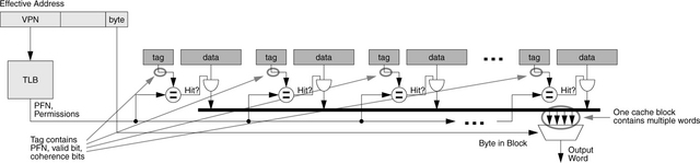
FIGURE 2.4 Fully associative lookup mechanism. This organization is also called a CAM, for content-addressable memory. It is similar to a database in that any entry that has the same tag as the lookup address matches, no matter where it is in the cache. This organization reduces cache contention, but the lookup can be expensive, since the tag of every entry is matched against the lookup address.
The benefit of a direct-mapped cache is that it is extremely quick to search and dissipates relatively little power, since there can only be one place that any particular datum can be found. However, this introduces the possibility that several different data might need to reside in the cache at the same place, causing what is known as contention for the desired data entry. This results in poor performance, with entries in the cache being replaced frequently; these are conflict misses. The problem can be solved by using a fully associative cache, a design choice traditionally avoided due to its high dynamic power dissipation (in a typical lookup, every single tag is compared to the search tag). However, as dynamic power decreases in significance relative to leakage power, this design choice will become more attractive.
• Set-Associative Organization: As a compromise between the two extremes, a set-associative cache lies in between direct-mapped and fully associative designs and often reaps the benefits of both designs—fast lookup and lower contention. Figures 2.5 and 2.6 illustrate two set-associative organizations. Figure 2.5 shows an implementation built of a small number of direct-mapped caches, typically used for low levels of set associativity, and Figure 2.6 shows an implementation built of a small number of content-addressable memories, typically used for higher degrees of set associativity.
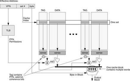
FIGURE 2.5 Block diagram for an n-way set-associative cache. A set-associative cache can be made of several direct-mapped caches operated in parallel. Note that data read-out is controlled by tag comparison with the TLB output as well as the block-valid bit (part of the tag or metadata entry) and the page permissions (part of the TLB entry). Note also that the cache column size is equal to the virtual memory page size (the cache index does not use bits from the VPN).
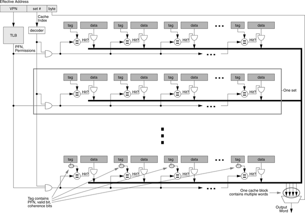
FIGURE 2.6 Set-associative cache built from CAMs. The previous figure showed a set-associative cache built of several direct-mapped caches, which is appropriate when the degree of associativity is low. When the degree of associativity is high, it is more appropriate to build the cache out of CAMs (content-addressable memories, i.e., fully associative caches), where each CAM represents one data set or equivalence class. For example, the Strong ARM’s 32-way set-associative cache is built this way.
These are the basic choices of organization for transparently addressed caches. They are applicable to solid-state implementations (evident from the diagrams) as well as software implementations. For instance, an operating system’s buffer cache or distributed memory system’s object cache could be implemented as a large array of blocks, indexed by a hash of the block ID or object ID, which would correspond to a direct-mapped organization as in Figure 2.3; it could be implemented as a binary search tree, which would correspond to a fully associative organization, because the search tree is simply software’s way to “search all tags in parallel” as in Figure 2.4; or it could be implemented as a set of equivalence classes, each of which maintains its own binary search tree, an arrangement that would correspond to a set-associative organization as in Figure 2.6 (each row in the figure is a separate equivalence class). The last organization of software cache could significantly reduce the search time for any given object, assuming that the assignment of objects to equivalence classes is evenly distributed.
An important point to note is that, because the transparently addressed cache uses the same namespace as the backing store, it is possible (and this is indeed the typical case) for the cache to maintain only a copy of the datum that is held in the backing store. In other words, caching an object does not necessarily supersede or invalidate the original. The original stays where it is, and it is up to the consistency-management solution to ensure that the original is kept consistent with the cached copy.
What does this have to do with logical organization? Because the transparently addressed cache maintains a copy of the object’s identifier (e.g., its physical address, if the backing store is main memory), it is possible for the cache to keep the copy in the backing store consistent transparently. Without this information, the application software must be responsible for maintaining consistency between the cache and the backing store. This is a significant issue for processor caches: if the cache does not maintain a physical tag for each cached item, then the cache hardware is not capable of ensuring the consistency of the copy in main memory.
From this point, transparently addressed caches are further divided, depending on whether their contents are managed implicitly (i.e., by the cache itself) or explicitly (i.e., by the application software).
2.2.1 Implicit Management: Transparent Caches
Transparent caches are the most common form of general-purpose processor caches. Their advantage is that they will typically do a reasonable job of improving performance even if unoptimized and even if the software is totally unaware of their presence. However, because software does not handle them directly and does not dictate their contents, these caches, above all other cache organizations, must successfully infer application intent to be effective at reducing accesses to the backing store. At this, transparent caches do a remarkable job.
Cache design and optimization is the process of performing a design-space exploration of the various parameters available to a designer by running example benchmarks on a parameterized cache simulator. This is the “quantitative approach” advocated by Hennessy and Patterson in the late 1980s and early 1990s [Hennessy & Patterson 1990]. The latest edition of their book is a good starting point for a thorough discussion of how a cache’s performance is affected when the various organizational parameters are changed. Just a few items are worth mentioning here (and note that we have not even touched the dynamic aspects of caches, i.e., their various policies and strategies):
• Cache misses decrease with cache size, up to a point where the application fits into the cache. For large applications, it is worth plotting cache misses on a logarithmic scale because a linear scale will tend to downplay the true effect of the cache. For example, a cache miss rate that decreases from 1% to 0.1% to 0.01% as the cache increases in size will be shown as a flat line on a typical linear scale, suggesting no improvement whatsoever, whereas a log scale will indicate the true point of diminishing returns, wherever that might be. If the cost of missing the cache is small, using the wrong knee of the curve will likely make little difference, but if the cost of missing the cache is high (for example, if studying TLB misses or consistency misses that necessitate flushing the processor pipeline), then using the wrong knee can be very expensive.
• Comparing two cache organizations on miss rate alone is only acceptable these days if it is shown that the two caches have the same access time. For example, processor caches have a tremendous impact on the achievable cycle time of the microprocessor, so a larger cache with a lower miss rate might require a longer cycle time that ends up yielding worse execution time than a smaller, faster cache. Pareto-optimality graphs plotting miss rate against cycle time work well, as do graphs plotting total execution time against power dissipation or die area.
• As shown at the end of the previous chapter, the cache block size is an extremely powerful parameter that is worth exploiting. Large block sizes reduce the size and thus the cost of the tags array and decoder circuit. The familiar saddle shape in graphs of block size versus miss rate indicates when cache pollution occurs, but this is a phenomenon that scales with cache size. Large cache sizes can and should exploit large block sizes, and this couples well with the tremendous bandwidths available from modern DRAM architectures.
2.2.2 Explicit Management: Software-Managed Caches
We return to the difference between transparent caches and scratch-pad memories. A program addresses a transparent cache implicitly, and the cache holds but a copy of the referenced datum. A program references a scratch-pad explicitly, and a datum is brought into the scratch-pad by an operation that effectively gives the item a new name. In essence, a load from the backing store, followed by a store into a scratch-pad, creates a new datum, but does not destroy the original. Therefore, two equal versions of the datum remain. However, there is no attempt by the hardware to keep the versions consistent (to ensure that they always have the same value) because the semantics of the mechanism suggest that the two copies are not, in fact, copies of the same datum, but instead two independent data. If they are to remain consistent, it is up to the application software to perform the necessary updates. As mentioned earlier, this makes scratch-pad memories less-than-ideal compiler targets, especially when compared to transparent caches. Round one to the transparent cache.
Because they could potentially hold anything in the backing store, transparent caches require tags to indicate what data is currently cached; scratch-pad memories require no tags. In solid-state implementations, tags add significant die area and power dissipation: a scratch-pad SRAM can have 34% smaller area and 40% lower power dissipation than a transparent cache of the same capacity [Banakar et al. 2002]. Round two to the scratch-pad.
General-purpose processor caches are managed by the cache hardware in a manner that is transparent to the application software. In general, any data item touched by the application is brought into the cache. In contrast, nothing is brought into the scratch-pad unless it is done so intentionally by the application software through an explicit load and store. The flip side of this is interesting. Whereas any reference can potentially cause important information to be removed from a traditional cache, data is never removed from a scratch-pad unless it is done so intentionally. This is why scratch-pads have more predictable behavior than transparent caches and why transparent caches are almost universally disabled in real-time systems, which value predictability over raw performance. Round three to the scratchpad, at least for embedded applications.
A hybrid solution that could potentially draw together two of the better aspects of caches and scratch-pads is an explicitly managed, transparently addressed cache, or software-managed cache [Jacob 1998]. Such a cache organization uses transparent addressing, which offers a better compiler target than explicit addressing, but the organization relies upon software for content management, an arrangement that allows one to ensure at design time what the cache’s contents will be at run time. In addition, the cache uses the same namespace as the backing store, and thus the cache can automatically keep its contents consistent with the backing store. As will be discussed in the next chapter, the cache can rely upon the programmer and/or compiler to decide what to cache and when to cache it, similar to scratch-pad memories. Note that this organization is not an all-around total-win situation because it still requires a tag store or similar function, and thus it is more expensive than a scratch-pad SRAM, at least in a solid-state implementation.
The following are examples of software-managed processor caches.
VMP: Software-Controlled Virtual Caches
The VMP multiprocessor [Cheriton et al. 1986, 1988, 1989] places the content and consistency management of its virtual caches under software control, providing its designers an extremely flexible and powerful tool for exploring coherence protocols. The design uses large cache blocks and a high degree of associativity to reduce the number of cache misses and therefore the frequency of incurring the potentially high costs of a software-based cache fill.
Each VMP processor node contains several hardware structures, including a central processing unit, a software-controlled virtual cache, a cache controller, and special memory (see Figure 2.7). Objects the system cannot afford to have causing faults, such as root page tables and fault-handling code, are kept in a separate area called local memory, distinguished by the high-order bits of the virtual address. Local memory is essentially a scratch-pad memory. Like SPUR (symbolic processing using RISCs) [Ritchie 1985, Hill et al. 1986], VMP eliminates the TLB, but instead of using a hardware table-walker, VMP relies upon a software handler maintained in this local memory. A cache miss invokes a fault handler that locates the requested data, possibly causes other caches on the bus to invalidate their copies, and loads the cache. Note that, even though the cache-miss handler is maintained in a separate cache namespace, it is capable of interacting with other software modules in the system.
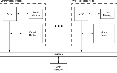
FIGURE 2.7 The VMP multiprocessor. Each VMP processor node contains a microprocessor (68020), local cache outside the namespace of main memory, and a software-controlled virtual cache. The software-controlled cache made the design space for multiprocessor cache coherency easier to explore, as the protocols could be rewritten at will.
An interesting development in VMP is the use of a directory structure for implementing cache coherence. Moreover, because the directory maintains both virtual and physical tags for objects (so that main memory can be kept consistent transparently), the directory structure also effectively acts as a cache for the page table. The VMP software architecture uses the directory structure almost to the exclusion of the page table for providing translations because it is faster, and using it instead of the page table can reduce memory traffic significantly. This enables the software handler to perform address translation as part of cache fill without the aid of a TLB, but yet quickly enough for high-performance needs. A later enhancement to the architecture [Cheriton et al., 1988] allowed the cache to do a hardware-based cache refill automatically, i.e., without vectoring to a software handler, in instances where the virtual-physical translation is found in the directory structure.
SoftVM: A Cache-Fill Instruction
Another software-managed cache design was developed for the University of Michigan’s PUMA project [Jacob & Mudge 1996, 1997, 2001]. It is very similar to Cheriton’s software-controlled virtual caches, with the interesting difference being the mechanism provided by the architecture for cache fill. The software cache-fill handler in VMP is given by the hardware a cache slot as a suggestion, and the hardware moves the loaded data to that slot on behalf of the software. PUMA’s SoftVM mechanism was an experiment to see how little hardware one could get away with (e.g., it maintains the handler in regular memory and not a separate memory, and like SPUR and VMP, it eliminates the TLB); the mechanism provides the bare necessities to the software in the form of a single instruction.2
When a virtual address fails to hit in the bottommost cache level, a cache-miss exception is raised. The address that fails to hit in the lowest level cache is the failing address, and the data it references is the failing data. On a cache-miss exception, the hardware saves the program counter of the instruction causing the cache miss and invokes the miss handler. The miss handler loads the data at the failing address on behalf of the user thread. The operating system must therefore be able to load a datum using one address and place it in the cache tagged with a different address. It must also be able to reference memory virtually or physically, cached or uncached. For example, to avoid causing a cache-miss exception, the cachemiss handler must execute using physical addresses. These may be cacheable, provided that a cacheable physical address that misses the cache causes no exception and that a portion of the virtual space can be directly mapped onto physical memory.
When a virtual address misses the cache, the failing data, once loaded, must be placed in the cache at an index derived from the failing address and tagged with the failing address’s virtual tag; otherwise, the original thread will not be able to reference its own data. A new load instruction is defined, in which the operating system specifies a virtual tag and set of protection bits to apply to the incoming data, as well as a physical address from which to load the data. The incoming data is inserted into the caches with the specified tag and protection information. This scheme requires a privileged instruction to be added to the instruction-set architecture: mapped-load, depicted in Figure 2.8.
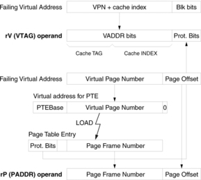
FIGURE 2.8 Mapped-load instruction. The top portion gives the syntax and semantics of the instruction. The bottom portion illustrates the source of the rV (VTAG+prot bits) and rP (physical address) operands. The example assumes an MIPS-like page table.
The mapped-load instruction is simply a load-to-cache instruction that happens to tell the virtual cache explicitly what bits to use for the tag and protection information. It does not load to the register file. It has two operands, as shown in the following syntax:
![]()
The protection bits in rV come from the mapping PTE. The VADDR portion of rV comes from the failing virtual address; it is the topmost bits of the virtual address minus the size of the protection information (which should be no more than the bits needed to identify a byte within a cache block). Both the cache index and cache tag are recovered from VADDR (virtual address); note that this field is larger than the virtual page number. The hardware should not assume any overlap between virtual and physical addresses beyond the cache line offset. This is essential to allow a software-defined (i.e., operating-system-defined) page size.
The rP operand is used to fetch the requested datum, so it can contain a virtual or physical address. The datum identified by the rP operand is obtained from memory (or perhaps the cache itself) and then inserted into the cache at the cache block determined by the VADDR bits and tagged with the specified virtual tag. Thus, an operating system can translate data that misses the cache; load it from memory (or even another location in the cache); and place it in any cache block, tagged with any value. When the original thread is restarted, its data is in the cache at the correct line with the correct tag. To restart the thread, the failing load or store instruction is retried.
![]()
The single mapped-load instruction is an atomic operation. The fact that the load is not binding (i.e., no data is brought into the register file) means that it does not actually change the processor state. Protections are not checked until the failing load or store instruction is retried, at which point it could be found that a protection violation occurred. This simplifies the hardware requirements. Because the data is not transferred to the register file until a failing load is retried, different forms of the mapped-load for load word, load halfword, load byte, etc. are not necessary. There is no compiler impact on adding the mapped-load to an instruction set because the instruction is privileged and will not be used by user-level instructions; it will be found only in the cache-miss handler which will most likely be written in assembly code.
2.3 Non-Transparently Addressed Caches
A non-transparently addressed cache is one that the application software must know about to use. The cache data lies in a separate namespace from the backing store, and the application must be aware of this namespace if it is to use the cache. The advantage of this arrangement is that a cache access requires no search, no lookup. There is no question whether the item requested is present in the cache because the item being requested is not an object from the backing store, but instead is a storage unit within the cache itself, e.g., the cache would be explicitly asked by application software for the contents of its nth storage block, which the cache would return without the need for a tag compare or key lookup. This has a tremendous impact on implementation. For instance, in solid-state technologies (e.g., SRAMs) this type of cache does not require the tag bits, dirty bits, and comparison logic found in transparently addressed caches.
A common example of non-transparently addressed caches is SRAM that is memory-mapped to a part of the address space (e.g., the SRAM0 and SRAM1 segments shown in Chapter 0, Figure 0.4) or storage that is accessed based on context (e.g., the internal and external data segments of the 8051 microcontroller, shown in Figure 2.9). Note that these arrangements exhibit an exclusive relationship with the backing store: an item is either in the scratch-pad or in the backing store, but it cannot be in both because their namespaces (enforced by requiring different access mechanisms) are disjoint.
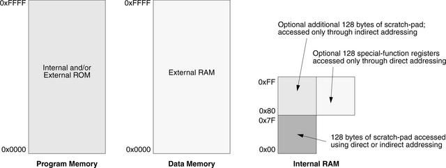
FIGURE 2.9 Memory map for the 8051 microcontroller. Program memory, which is either internal or external ROM, is accessed on instruction-fetch; data memory, external RAM, is accessed through MOVX instructions; and internal RAM is accessed using indirect and/or direct addressing. [Synopsys 2002]
Because there is no need for a potentially expensive search in this type of cache, many of the different choices of organization for transparently addressed caches become obviated, and in practice, many non-transparent caches are simply large arrays of storage blocks. However, because the cost of reading the cache can be significant both in access time and in power dissipation as the cache gets large, the cache is typically partitioned into subordinate banks, only one of which is activated on a read or write. This partitioning can be transparent or exposed to the application software. A transparent example would be an SRAM divided in 2n banks, one of which is chosen by an n-bit vector taken from the cache address. On the other hand, one would want to expose the partition to software if, for example, the partitions are not all equal in size or cost of access, in which case a compiler-based heuristic could arrange cached data among the various partitions according to weights derived from the partitions’ associated costs.
An important point to note is that, because the cache uses a namespace that is separate from the backing store, the cache exhibits an exclusive relationship with the backing store; that is, the cache, by definition, does not maintain a copy of the datum in the backing store, but instead holds a separate datum entirely. Moving data into an explicitly addressed cache creates a brand-new data item, and unless the cache is given a pointer to the original in the backing store, the cache cannot automatically maintain consistency between the version in the cache and the version in the backing store.
From this point, explicitly addressed caches are further divided, depending on whether their contents are managed explicitly (i.e., by the application software) or implicitly (i.e., by the cache itself).
2.3.1 Explicit Management: Scratch-Pad Memories
Scratch-pad memory (SPM) offers the ultimate in application control. It is explicitly addressed, and its contents are explicitly managed by the application software. Its data allocation is meant to be done by the software, usually the compiler, and thus, like software-managed caches, it represents a more predictable form of caching that is more appropriate for real-time systems than caches using implicit management.
The major challenge in using SPMs is to allocate explicitly to them the application program’s frequently used data and/or instructions. The traditional approach has been to rely on the programmer, who writes annotations in source code that assign variables to different memory regions. Program annotations, however, have numerous drawbacks.
• They are tedious to derive and, like all things manual in programming, are fraught with the potential for introducing bugs.
• A corollary to the previous point: they increase software development time and cost.
• They are not portable across memory sizes (they require manual rewriting for different memory sizes).
• They do not adapt to dynamically changing program behavior.
For these reasons, programmer annotations are increasingly being replaced by automated, compile-time methods. We will discuss such methods in the next chapter.
Perspective: Embedded vs. General-Purpose Systems
As mentioned earlier, transparent caches can improve code even if that code has not been designed or optimized specifically for the given cache’s organization. Consequently, transparent caches have been a big success for general-purpose systems, in which backward compatibility between next-generation processors and previous-generation code is extremely important (i.e., modern processors are expected to run legacy code that was written with older hardware in mind). Continuing with this logic, using SPM is usually not even feasible in general-purpose systems due to binary-code portability: code compiled for the scratchpad is usually fixed for one SRAM size. Binary portability is valuable for desktops, where independently distributed binaries must work on any cache size. In many embedded systems, however, the software is usually considered part of the co-design of the system: it resides in ROM and cannot be changed. Thus, there is really no harm to having embedded binaries customized to a particular memory size. Note that source code is portable even though a specific executable is optimized for a particular SRAM size; recompilation with a different memory size is always possible.
Though transparent caches are a mainstay of general-purpose systems, their overheads are less defensible for use in embedded systems. Transparent caches incur significant penalties in area cost, energy, hit latency, and real-time guarantees. Other than hit latency, all of these are more important for embedded systems than for general-purpose systems. A detailed recent study compares transparent caches with SPMs. Among other things, they show that a scratchpad has 34% smaller area and 40% lower power consumption than a cache of the same capacity [Banakar et al. 2002]. These savings are significant since the on-chip cache typically consumes 25–50% of the processor’s area and energy consumption, a fraction that is increasing with time. More surprisingly, Banakar compares performance of a transparent cache to that of a scratch-pad using a simple static knapsack-based allocation algorithm and measures a run-time cycle count that is 18% better for the scratch-pad. Defying conventional wisdom, they found no advantage to using a transparent cache, even in high-end embedded systems in which performance is important.
Given the power, cost, performance, and real-time advantages of a scratch-pad, it is not surprising that scratch-pads are the most common form of SRAM in embedded CPUs today. Examples of embedded processors with a scratch-pad include low-end chips such as the Motorola MPC500, Analog Devices ADSP-21XX, and Motorola Coldfire 5206E; mid-grade chips such as the ARMv6, Analog Devices ADSP-21160m, Atmel AT91-C140, ARM 968E-S, Hitachi M32R-32192, and Infineon XC166; and high-end chips such as Analog Devices ADSP-TS201S, Hitachi SuperH-SH7050, IBM’s PowerPC 405/440, and Motorola Dragonball. In addition, high-performance chips for games and other media applications, such as IBM’s new Cell Architecture, and network processors, such as the Intel’s IXP network processor family, all include SPm.
Trends in recent embedded designs indicate that the dominance of a scratch-pad will likely consolidate further in the future [LCTES Panel 2003, Banakar et al. 2002] for regular processors as well as network processors.
2.3.2 Implicit Management: Self-Managed Scratch-Pads
The implicitly managed, non-transparent memory, or self-managed scratch-pad, is an odd beast. Due to the cache’s non-transparent addressing scheme, the cache data lies in its own namespace, and therefore, the cache exhibits an exclusive relationship with the backing store. It does not hold copies of the data, but the actual data themselves. This could be useful in a secure setting or one in which storage space is at a premium. The cache contents are decided by the cache’s heuristics, not the application software. This provides cross-compatibility to support software not explicitly written for the cache in question, and it makes for a better compiler target than an explicitly managed cache.
Such a cache model would make sense, for example, in a distributed shared memory system in which objects are not allowed to have multiple copies lying around the system (e.g., Emerald’s mobile objects [Jul et al. 1988]), the local space and global storage use different namespaces (e.g., permanent object stores that perform swizzling [Hosking & Moss 1990]), and the underlying caching architecture performs the cache fill automatically on behalf of the application.
2.4 Virtual Addressing and Protection
Virtual addressing is available for solid-state cache implementations in systems with virtual memory support. Generally, the concept is also applicable beyond solid-state implementations and simply implies that one can create a new namespace orthogonal to that of the backing store and local cache storage and perform some mapping between. However, we will stick to the solid-state version, largely because this serves as a foundation for the many problems that virtual memory creates and must be solved.
By “protection” we are referring to the general mechanism that the operating system uses to protect data from misuse, e.g., overwriting text pages, gaining access to the data of another process, etc. The operating system cannot be involved in every memory access, and one efficient alternative is to provide the appropriate support in the cache system.
Note that these mechanisms are not specific to explicit/implicit addressing or explicit/implicit management. Virtual caches, address-space identifiers (ASIDs), and/or protection bits can all be used in any of the cache organizations described in this chapter.
2.4.1 Virtual Caches
As mentioned earlier, a transparent cache is an implementation in which the stored object retains the same identifier as is used to access it from the backing store. Virtual caches offer a slight twist on this idea. The backing store for a processor cache is usually taken to be main memory, physically addressed; therefore, one would expect all processor caches to use the physical address to identify a cached item. However, virtual memory offers a completely different address for use, one which might be even more convenient to use than the physical address. Recall that on each cache access, the cache is indexed, and the tags are compared. For each of these actions, either the data block’s virtual address or the data block’s physical address may be used. Thus, we have four choices for cache organization.
Physically indexed, physically tagged: The cache is indexed and tagged by its physical address. Therefore, the virtual address must be translated before the cache can be accessed. The advantage of the design is that since the cache uses the same namespace as physical memory, it can be entirely controlled by hardware, and the operating system need not concern itself with managing the cache. The disadvantage is that address translation is in the critical path. This becomes a problem as clock speeds increase, as application data sets increase with increasing memory sizes, and as larger TLBs are needed to map the larger data sets (it is difficult and expensive to make a large TLB fast). Two different physically indexed, physically tagged organizations are illustrated in Figure 2.10. The difference between the two is that the second uses only bits from the page offset to index the cache, and therefore its TLB lookup is not in the critical path for cache indexing (as it is in the first organization).
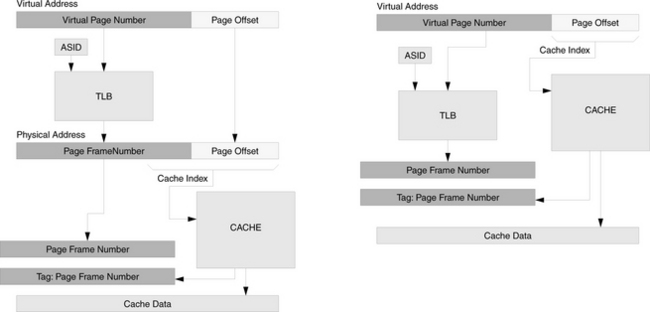
FIGURE 2.10 Two physically indexed, physically tagged cache organizations. The cache organization on the right uses only bits from the page offset to index the cache, and so it is technically still a virtually indexed cache. The benefit of doing so is that its TLB lookup is not in the critical path for cache indexing (as is the case in the organization on the left). The disadvantage is that the cache index cannot grow, and so cache capacity can only grow by increasing the size of each cache block and/or increasing set associativity.
Physically indexed, virtually tagged: The cache is indexed by its physical address, but the tag contains the virtual address. This is traditionally considered an odd combination, as the tag is read out as a result of indexing the cache. If the physical address is available at the start of the procedure (implying that address translation has been performed), then why not use the physical address as a tag? If a single physical page is being shared at two different virtual addresses, then there will be contention for the cache line, since both arrangements cannot be satisfied at the same time. However, if the cache is the size of a virtual page, or if the size of the cache bin (the size of the cache divided by its associativity [Kessler & Hill 1992]) is no more than a virtual page, then the cache is effectively indexed by the physical address since the page offset is identical in the virtual and physical addresses. This organization is pictured in Figure 2.11 on the left. The advantage of the physically indexed, virtually tagged cache organization is that, like the physically indexed/physically tagged organization, the operating system need not perform explicit cache management. On the right is an optimization that applies to this organization as well as the previous organization. To index the cache with a physical address, not all of the virtual page bits need translation; only those that index the cache need translation. The MIPS R6000 used what they called a TLB Slice to translate only the small number of bits needed for cache access [Taylor et al. 1990]. The “translation” obtained is only a hint and not guaranteed to be correct. Thus, it uses only part of the VPN and does not require an ASId.
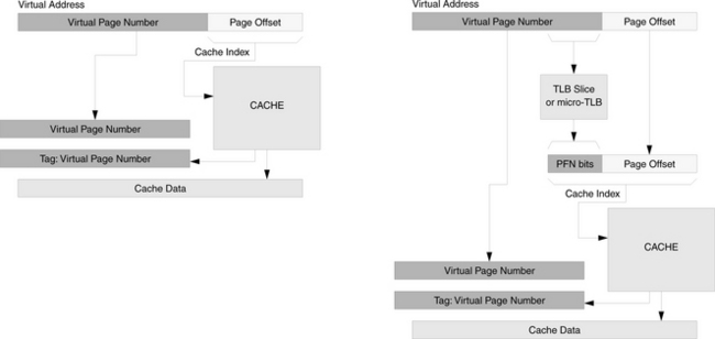
FIGURE 2.11 Two physically indexed, virtually tagged cache organizations. The cache organization on the left uses only bits from the page offset to index the cache. It is technically still a virtually indexed cache. As shown on the right, one need not incur the cost of accessing the entire TLB to get a physical index; one need only translate enough bits to index the cache.
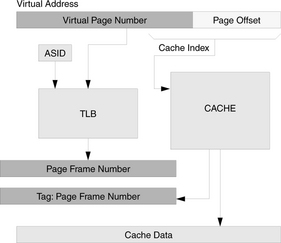
Virtually indexed, physically tagged: The cache is indexed by the virtual address, which is available immediately since it needs no translation, and the cache is tagged by the physical address, which does require translation. Since the tag compare happens after indexing the cache, the translation of the virtual address can happen at the same time as the cache index; the two can be done in parallel. Though address translation is necessary, it is not in the critical path. The advantages of the scheme are a much faster access time than a physically indexed cache and a reduced need for management as compared to a virtually indexed, virtually tagged cache (e.g., hardware can ensure that multiple aliases to the same physical block do not reside in multiple entries of a set). However, management is still necessary, as opposed to physically indexed caches, because the cache is virtually indexed. The cache organization is illustrated in Figure 2.12.
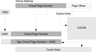
Virtually indexed, virtually tagged: The cache is indexed and tagged by the virtual address. The advantage of this design is that address translation is not needed anywhere in the process. A translation lookaside buffer is not needed, and if one is used, it only needs to be accessed when a requested datum is not in the cache. On such a cache miss, the operating system must translate the virtual address and load the datum from physical memory. A TLB would speed up the translation if the translation had been performed previously and the mapping was still to be found in the TLB. Since the TLB is not in the critical path, it could be very large; though this would imply a slow access time, a larger TLB would hold much more mapping information, and its slow access time would be offset by its infrequency of access. The cache organization is illustrated in Figure 2.13.
Why might one of these organizations be more convenient than another? One can clearly see that the TLB, if involved, is an essential component of cache lookup. In a large, physically indexed cache, the TLB lookup is on the critical path to cache access: the cache cannot be accessed until the TLB returns the physical translation. Either both lookups (TLB probe and cache probe) must be fast enough to fit together, sequentially, in a single clock cycle or the two must be pipelined on successive cycles, which pushes cache access out a cycle later than when the target address first becomes available. Using the virtual index (or constraining the size of the cache so that the cache index is the same bit vector in both the virtual and physical addresses, as in the right-hand side of Figure 2.10) moves the TLB lookup off the critical path, thereby speeding up the cache access.
For another example, note that a cache hit relies upon a TLB hit (for the tag as well as page-level access permissions). Instances exist in which the requested data is found in the cache, but its corresponding mapping information is not found in the TLB. These cases represent de facto cache misses because, in these cases, the cache access cannot proceed until the TLB is refilled [Jacob & Mudge 1997, 2001]. In virtually tagged caches (Figures 2.11 and 2.13), the TLB probe is not needed until a cache miss occurs, an event that is infrequent for large caches. These cache organizations can accept a TLB that is expensive (i.e., slow and/or power inefficient) because the TLB is rarely probed—as opposed to cache organizations with physical tags, in which the TLB is probed on every cache access.
However, removing the TLB from the equation is very tricky. For instance, if the cache uses a virtual tag, then the cache must be direct-mapped or managed by the client (e.g., the operating system). The use of a virtual tag implies that the cache itself will not be able to distinguish between multiple copies of the same datum if each copy is labeled with a different virtual address. If a physical region is accessed through multiple virtual addresses, then a set-associative cache with only virtual tags would allow the corresponding cache data to reside in multiple locations within the cache—even within multiple blocks of the same set.
Note that, though virtual addressing is compatible with both explicit and implicit cache management, if a virtual cache is expected to maintain data consistency with the backing store, the cache’s organization must contain for each stored block its identifier from the backing store (e.g., a physical tag for a solid-state implementation). If the cache has no back-pointer, it will be incapable of transparently updating the backing store, and such consistency management will necessarily be the software’s responsibility.
2.4.2 ASIDs and Protection Bits
ASIDs and protection bits are means for the cache to enforce the operating system’s protection designation for blocks of data. An operating system that implements multi-tasking will assign different IDs to different tasks to keep their associated data structures (e.g., process control blocks) separate and distinct. Operating systems also keep track of page-level protections, such as enforcing read-only status for text pages and allowing data pages to be marked as read-only, read/write, or write-only, for example, to implement safely a unidirectional communication pipe between processes through shared memory segments.
Some issues that arise include distinguishing the data of one process from the data belonging to another process once the data are cached. Numerous simple solutions exist, but the simple solutions are often inefficient. For example, one could use no ASIDs in the cache system and flush the caches on context switches and operating-system traps. One could use no protection bits in the cache system and avoid caching writable data, instead flushing all write data immediately to the backing store. Obviously, using the cache system to perform these functions is appropriate, and if the cache system is to enforce protection, it must maintain ASIDs and protection bits.
Address space identification within the cache is implicit if the cache is physically tagged—using physical tags pushes the burden of differentiating processes onto the shoulders of the virtual memory system (e.g., via the TLB, which takes an ASID as input, or via the page table, which effectively does the same). However, if the cache is virtually tagged, an ASID must be present, for example, in each tag.
Protection bits are necessary for both virtual and physical caches, unless the function is provided by the TLB. If so, note that read/write protection is provided at a page-level granularity, which precludes a block- or sub-block-level protection mechanism, both of which have been explored in multiprocessor systems to reduce false sharing.
2.4.3 Inherent Problems
Virtual caches complicate support for virtual-address aliasing and protection-bit modification. Aliasing can give rise to the synonym problem when memory is shared at different virtual addresses [Goodman 1987], and this has been shown to cause significant overhead [Wheeler & Bershad 1992]. Protection-bit modification is used to implement such features as copy-on-write [Anderson et al. 1991, Rashid et al. 1988] and can also cause significant overhead when used frequently.
The synonym problem has been solved in hardware using schemes such as dual tag sets [Goodman 1987] or back-pointers [Wang et al. 1989]. Synonyms can be avoided completely by setting policy in the operating system. For example, OS/2 requires all shared segments to be located at identical virtual addresses in all processes so that processes use the same address for the same data [Deitel 1990]. SunOS requires shared pages to be aligned in virtual space on extremely large boundaries (at least the size of the largest cache) so that aliases will map to the same cache line3 [Cheng 1987]. Single address space operating systems such as Opal [Chase et al. 1992a and b] or Psyche [Scott et al. 1988] solve the problem by eliminating the need for virtual-address aliasing entirely. In a single address space, all shared data is referenced through global addresses. As in OS/2, this allows pointers to be shared freely across process boundaries.
Protection-bit modification in virtual caches can also be problematic. A virtual cache allows one to “lazily” access the TLB only on a cache miss. If this happens, protection bits must be stored with each cache line or in an associated page-protection structure accessed every cycle, or else protection is ignored. When one replicates protection bits for a page across several cache lines, changing the page’s protection can be costly. Obvious but expensive solutions include flushing the entire cache or sweeping through the entire cache and modifying the affected lines.
A problem also exists with ASIDs. An operating system can maintain hundreds or thousands of active processes simultaneously, and in the course of an afternoon, it can sweep through many times that amount. Each one of these processes will be given a unique identifier, because operating systems typically use 32-bit or 64-bit numbers to identify processes. In contrast, many hardware architectures only recognize tens to hundreds of different processes [Jacob & Mudge 1998b]—MIPS R2000/3000 has a 6-bit ASID; MIPS R10000 has an 8-bit ASID; and Alpha 21164 has a 7-bit ASId. In these instances, the operating system will be forced to perform frequent remapping of ASIDs to process IDs, with TLB and cache flushes required for every remap (though, depending on implementation, these flushes could be specific to the ASID involved and not a whole-scale flush of the entire TLB and/or cache). Architectures that use IBM 801-style segmentation [Chang & Mergen 1988] and/or larger ASIDs tend to have an easier time of this.
2.5 Distributed and Partitioned Caches
Numerous cache organizations exist that are not monolithic entities. As mentioned earlier, the primary concern is convenience when analyzing these caches. For example, a level-1 cache may comprise a dedicated instruction cache and another dedicated data cache. In some instances, it is convenient to refer to “the level-1 cache” as a whole (e.g., “the chip has a 1MB L1 cache”), while in other instances it conveys more information to refer to each individual part of the cache (e.g., “the L1 i-cache has a 10% hit rate, while the L1 d-cache has a 90% hit rate,” suggesting a rebalancing of resources). Note that the constituent components ganged together for the sake of convenience need not lie at the same horizontal “level” in the memory hierarchy (as illustrated in Chapter 1, Figures 1.8 and 1.9). A hierarchical web cache can be described and analyzed as “a cache” when, in fact, it is an entire subnetwork of servers organized in a tiered fashion and covering a large physical/geographical expanse.
Generally speaking, the smallest thing that can be called a cache is the smallest addressable unit of storage—a unit that may or may not be exposed externally to the cache’s client. For example, within a multi-banked, solid-state cache, the bank is the smallest addressable unit of storage (note that a common metric for measuring cache behavior is the degree of “bank conflicts”), but the bank is usually not directly addressable by the cache’s client. As another example, web proxies can be transparent to client software, in which case the client makes a request to the primary server and the request is caught by or redirected to a different server entirely. The bottom line is that the constituent components of a cache or cache system may or may not be addressable by the cache’s clients. In other words, the various internal partitions of the cache are typically treated as implementation details and are not usually exposed to client software. However, one might want to expose the internal partitions to client software if, for example, the partitions are not all equal in size or cost of access. Note that web caching comes in several different flavors. Proxy servers can be hidden, as described above, but they can just as easily be exposed to client software and even to the human using the web browser, as in the case of mirror sites for downloads, in which case the human typically chooses the nearest source for the desired data. The process can be automated. For instance, if a solid-state cache’s partitions are exposed to software and exhibit different behaviors (cost of access, cost of storage, etc.), a compiler-based heuristic could arrange cached data among the various partitions according to weights derived from the partitions’ associated costs. An extremely diverse range of heuristics has been explored in both software and hardware to do exactly this (see Chapter 3, “Management of Cache Contents”).
The following sections describe briefly some common distributed and/or partitioned cache organizations.
2.5.1 UMA and NUMA
UMA and NUMA stand for uniform memory access and non-uniform memory access, respectively. The terms are most often used in the context of higher order memory systems and not specifically cache systems, but they are useful designations in the discussion of distributed/partitioned caches because UMA/NUMA systems illustrate the main issues of dealing with physically disjoint memories. A NUMA architecture is one in which all memory accesses have nominally the same latency; a NUMA architecture is one in which references to different addresses may have different latencies due to the nature of where the data is stored. The implication behind the deceptively simple “where the data is stored” is that an item’s identity is tied to its location. For instance, in a solid-state setting, an item’s physical address determines the memory partition in which it can be found. As an example, in a system of 16 memory nodes, the physical memory space could be divided into 16 regions, and the top 4 bits of the address would determine which node owns the data in question.
Figure 2.14(a) shows an organization in which a CPU’s requests all go to the same memory system (which could be a cache, the DRAM system, or a disk; the details do not matter for purposes of this discussion). Thus, all memory requests have nominally the same latency—any observed variations in latency will be due to the specifics of the memory technology and not the memory organization. This organization is typical of shared cache organizations (e.g., the last-level cache of a chip-level multiprocessor) and symmetric multiprocessors.
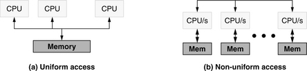
Figure 2.14(b) shows an organization in which a CPU’s memory request may be satisfied by one of many possible sub-memories. In particular, a request to any non-local memory (any memory not directly attached to the CPU making the request) is likely to exhibit a higher latency than a request to a local memory. This organization is used in many commercial settings, such as those based on AMD Opteron or Alpha 21364 (EV7) processors. The ccNUMA variant (for cache-coherent NUMA) is one in which each processor or processor cluster maintains a cache or cache system that caches requests to reduce internode traffic and average latency to non-local data.
The concepts embodied in the terms UMA and NUMA extend to cache systems and memory systems in general because the issues are those of data partitioning and placement, cost/benefit analysis, etc., which are universal. The Fully Buffered DIMM is a prime example of a non-uniform memory architecture which can be configured to behave as a uniform architecture by forcing all DIMMs in the system to stall and emulate the latency of the slowest DIMM in the system. For more detail, see Chapter 14, “The Fully Buffered DIMM Memory System.”
2.5.2 COMA
COMA stands for cache-only memory architecture, an organization designed to address the issues of UMA and NUMA and ccNUMA machines [Hagersten et al. 1992]. UMA organizations are not scalable beyond a relatively small number of nodes per memory; the shared-bus traffic quickly becomes a limiter to system performance. In NUMA organizations, the static assignment of data to partition creates unnecessary network traffic in the (frequent) case that the software working on the data happens to be running on a non-local processor. Even with caches at each compute node in a NUMA organization (ccNUMA), the problem is not necessarily solved. In high-performance applications, data sets can easily exceed the limited cache space.
COMA organizations were proposed to solve the problem by blurring the distinction between cache and backing store, making the local cache effectively the same size as the local backing store (DRAM system). A COMA organization is a distributed system of compute nodes that treats the DRAM space as a large cache, called an attraction memory. The idea is that the organization does the job of data partitioning for the software dynamically: as software threads run on different compute nodes, they attract to their node’s local memory all code they need and data on which they are working. In instances with little write-sharing of data, after an initial flurry of network activity, there is little memory traffic on the network.
There are two primary implications of this organization: one an advantage, the other a disadvantage. The advantage is a dramatically increased local cache space, which potentially reduces latency significantly. The disadvantage is that, by definition (“cache only”), there is no backing store, and thus, the system must keep track of extant cached copies so that they are not all deleted from the system. This complicates the cache-coherence mechanism. In addition, the fact that DRAM is treated as a cache implies that a tag feature must be added. This can be done through the virtual memory system (as pointed out, the virtual memory system treats main memory as an associative cache for the disk space), but it is limited by the reach of the TLB, meaning that if the TLB maps 4 KB per entry and has 256 entries, then at any given moment it can map a total of 1 MB of space (i.e., translate to physical addresses, or in the context of COMA, perform the tag-compare function). Anything outside of that space will require a page table traversal and TLB refill. Alternatively, the tag-compare function can be performed by special hardware (e.g., use a non-standard DRAM bus and store tag information with every block of memory), but this would increase the cost of the system.
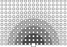
2.5.3 NUCA and NuRAPID
Figure 2.15 illustrates some recent perspectives on distributed/partitioned caches. The NUCA and NuRAPID (non-uniform access with replacement and placement using distance associativity) [Kim et al. 2002, Chishti et al. 2003] organizations gather together a set of storage nodes on a network-on-chip that is collectively called a monolithic cache, but which behaves as a de facto cache hierarchy, exhibiting different access latencies depending on the distance from the central access point and supporting the migration of data within the cache. The argument for treating the cache as a monolothic entity is that large on-chip caches already exhibit internal latencies that differ depending on the block being accessed. Another treatment of the cache would be to consider it as an explicit non-inclusive partition and use naming of objects for assignment to different sets within the cache, with the sets being grouped by similar latencies. One could locate data within the cache and schedule accesses to the cache using schemes similar to Abraham et al. [1993].
2.5.4 Web Caches
A good example of a distributed cache is the increasingly common web cache [Luotonen & Altis 1994] pictured in Figure 2.16 (note that the figure shows several different types of caches within a larger context of web infrastructure). First, each browser typically manages its own local cache in the client machine’s file system (which itself is cached by the operating system in an in-memory buffer cache). Second, the web server’s files are cached within the buffer cache of its operating system (and there is even a cache within the disk drive pictured). Finally, two different web caches are pictured. Web cache (a) is a server-side network of proxies put in place to reduce load on the main web server. The server-side cache increases system throughput and reduces average latency to clients of the system (i.e., customers). This type of cache can also reduce exposure to security problems by allowing the main bulk of an organization’s computing facilities, including the primary web server, to remain behind a firewall. Web cache (b) is a client-side cache put in place to reduce the traffic on an organization’s outgoing link to the network, thereby improving all traffic in general—queries satisfied by the cache appear to have very low latency, and, if the web cache has a high hit rate, other queries (including non-web traffic) see improved latency and bandwidth because they face less competition for access to the network.
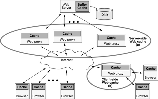
FIGURE 2.16 Web cache organization. Web cache (a) is put in place by the administrator of the server to reduce exposure to security issues (e.g., to put only proxies outside a firewall) and/or to distribute server load across many machines. Web cache (b) is put in place by the administrator of a subnet to reduce the traffic on its Internet link; the cache satisfies many of the local web requests and decreases the likelihood that a particular browser request will leave the local subnet.
As Figure 2.16 shows, web caches are installed at various levels in the network, function at several different granularities, and provide a wide range of different services. Thus, it should be no surprise that each distinct type of web cache has its own set of issues. The universal issues include the following:
• The data is largely read-only. Inclusive caches have an advantage here because read-only data can be removed from the cache at any time without fear of consistency problems. All lessons learned from instruction-delivery in very large multiprocessor machines are applicable (e.g., broadcast, replication, etc.), but the issue is complicated by the possibility of data becoming invalid from the server side when documents are updated with new content.
• The variable document size presents a serious problem in that a heuristic must address two orthogonal issues: (i) should the document in question be cached? and (ii) how best to allocate space for it? There is no unit-granularity “block size” to consider other than “byte,” and therefore replacement may involve removing more than one document from the cache to make room for an incoming document. Given that simple replacement (as in solid-state caches and buffer caches) is not an entirely closed question, complicating it further with additional variables is certain to make things difficult: witness the extremely large number of replacement policies that have been explored for web caches, and the issue is still open [Podlipnig & Böszörményi 2003].
Furthermore, the issues for client-side and server-side web caches can be treated separately.
Client-Side Web Caches
Client-side caches are transparent caches: they are transparently addressed and implicitly managed. The client-side web cache is responsible for managing its own contents by observing the stream of requests coming from the client side. All lessons learned from the design of transparent caches (e.g., the solid-state caches used in microprocessors and general-purpose computing systems) are applicable, including the wide assortment of partitioning and prefetching heuristics explored in the literature (see, for example, Chapter 3, Section 3.1.1, “On-Line Partitioning Heuristics,” and Section 3.1.2, “On-Line Prefetching Heuristics”).
Invalidation of data is an issue with these caches, but because the primary web server does not necessarily know of the existence of the cache, invalidation is either done through polling or timestamps. In a polling scenario, the client-side cache, before serving a cached document to a requesting browser, first queries the server on the freshness of its copy of the document. The primary server informs the proxy of the latest modification date of the primary copy, and the proxy then serves the client with the cached copy or a newly downloaded copy. In a timestamp scenario, the primary server associates a time-to-live (TTL) value with each document that indicates the point in time when the document’s contents become invalid, requiring a proxy to download a new copy. During the window between the first download and TTL expiration, the proxy assumes that the cached copy is valid, even if the copy at the primary server is, in fact, a newer updated version.
Server-Side Web Caches
Like client-side caches, server-side web caches are also transparently addressed, but their contents can be explicitly managed by the (administrators of the) primary web server. Thus, server-side web caches can be an example of a software-managed cache. Not all server-side web caches are under the same administrative domain as the primary server. For example, country caches service an entire domain name within the Internet namespace (e.g., *.it or *.ch or *.de), and because they cache documents from all web servers within the domain name, they are by definition independent from the organizations owning the individual web servers. Thus, server-side web caches can also be transparent.
In these organizations, the issue of document update and invalidation is slightly more complicated because, when the web cache and primary server are under the same administrative domain, mechanisms are available that are not possible otherwise. For instance, the cache can be entirely under the control of the server, in which case the server pushes content out to the caches, and the cache need not worry about document freshness. Otherwise, the issues are much the same as in client-side caches.
2.5.5 Buffer Caches
Figure 2.16 illustrates software caching of data. Figure 2.17 shows in more detail how the operating system is involved. Note that data is cached on both the operating system side and the disk side, which implements its own DRAM-resident cache for data. This can be thought of as a client-side cache (at the operating system level) and a server-side cache (at the disk level); the issues of partitioning the management heuristics are very similar to those in web cache design. Note that this is easily analyzed as a distributed cache, even though the constituent components are currently implemented independently. It is always possible (and, indeed, it has been proposed) to merge the management of the two caches into a single control point. Chapter 22 will go into the details of disk caching, and the next section gives a case study of the buffer cache in BSD (Berkeley Software Distributions) Unix.

2.6 Case Studies
The following sections present some well-known examples of cache organizations to illustrate the principles described in this chapter.
2.6.1 A Horizontal-Exclusive Organization: Victim Caches, Assist Caches
As an example of an exclusive partition on a horizontal level, consider Jouppi’s victim cache [1990], a small cache with a high degree of associativity that sits next to another, larger cache that has limited set associativity. The addition of a victim cache to a larger main cache allows the main cache to approach the miss rate of a cache with higher associativity. For example, Jouppi’s experiments show that a direct-mapped cache with a small fully associative victim cache can approach the miss rate of a two-way set associative cache.
The two caches in a main-cache-victim-cache pair exhibit an exclusive organization: a block is found in either the main cache or in the victim cache, but not in both. In theory, the exclusive organization gives rise to a non-trivial mapping problem of deciding which cache should hold a particular datum, but the mechanism is actually very straightforward as well as effective. The victim cache’s contents are defined by the replacement policy of the main cache; that is, the only data items found within the victim cache are those that have been thrown out of the main cache at some point in the past. When a cache probe, which looks in both caches, finds the requested block in the victim cache, that block is swapped with the block it replaces in the main cache. This swapping ensures the exclusive relationship. One of many variations on this theme is the HP-7200 assist cache [Chan et al. 1996], whose design was motivated by the processor’s automatic stride-based prefetch engine: if too aggressive, the engine would prefetch data that would victimize soon-to-be-used cache entries. In the assist cache, the incoming prefetch block is loaded not into the main cache, but instead into the highly associative cache and is then promoted into the main cache only if it exhibits temporal locality by being referenced again soon. Blocks exhibiting only spatial locality are not moved to the main cache and are replaced to main memory in a FIFO fashion. These two management heuristics are compared later in Chapter 3 (see “Jouppi’s Victim Cache, HP-7200 Assist Cache” in Section 3.1).
By adding a fully associative victim cache, a direct-mapped cache can approach the performance of a two-way set-associative cache, but because the victim cache is probed in parallel with the main cache, this performance boost comes at the expense of performing multiple tag comparisons (more than just two), which can potentially dissipate more dynamic power than a simple two-way set-associative cache. However, the victim cache organization uses fewer transistors than an equivalently performing set-associative cache, and leakage is related to the total number of transistors in the design (scales roughly with die area). Leakage power in caches is quickly outpacing dynamic power, so the victim cache is likely to become even more important in the future.
As we will see in later sections, an interesting point on the effectiveness of the victim cache is that there have been numerous studies of sophisticated dynamic heuristics that try to partition references into multiple use-based streams (e.g., those that exhibit locality and so should be cached, and those that exhibit streaming behavior and so should go to a different cache or no cache at all). The victim cache, a simpler organization embodying a far simpler heuristic, tends to keep up with the other schemes to the point of outperforming them in many instances [Rivers et al. 1998].
A cache organization (and management heuristic) similar to the victim cache is implemented in the virtual memory code of many operating systems. A virtual memory system maintains a pool of physical pages, similar to the I/O system’s buffer cache (see discussion of BSD below). The primary distinction between the two caches is that the I/O system is invoked directly by an application and thus observes all user activity to a particular set of pages, whereas the virtual memory system is transparent—invoked only indirectly when translations are needed—and thus sees almost no user-level activity to a given set of pages. Any access to the disk system is handled through a system call: the user application explicitly invokes a software routine within the operating system to read or write the disk system. In the virtual memory system, a user application accesses the physical memory directly without any assistance from the operating system, except in the case of TLB misses, protection violations, or page faults. In such a scenario, the operating system must be very clever about inferring application intent because, unlike the I/O system, the virtual memory system has no way of maintaining page-access statistics to determine each page’s suitability for replacement (e.g., how recently and/or frequently has each page been referenced).
Solutions to this problem include the clock algorithm and other similar algorithms [Corbato 1968, Bensoussan et al. 1972, Carr & Hennessy 1981], in which pages are maintained in an LRU fashion based upon hardware providing a use bit for each page, a per-page indicator set by hardware whenever its corresponding page has been accessed. The clock algorithm periodically walks the list of pages and marks them ready for replacement if they have not been used recently. Modern processor architectures do not typically support a use bit because the per-page reference information has traditionally been communicated to the operating system by the hardware modifying the page table directly (e.g., Bensoussan et al. [1972]), which is currently considered an extravagant overhead. However, modern architectures do support protection bits, and so the clock algorithm is often approximated in modern operating systems by tagging a page as non-readable and setting an appropriate bit when the operating system’s page-protection-violation handler is invoked upon the page’s first reference. If, within a period of time, the page has not been accessed, the handler is not invoked, and the corresponding bit does not get set. In the MIPS R2000 port of Mach, this mechanism is implemented through a set of queues: a page in the system is found on one of several queues based upon how recently it has been referenced on each period (execution of the clock algorithm), all unused pages are migrated one hop toward the available queue, and all referenced pages are moved onto the in-use queue. Thus, a physical page has several periods to prove its usefulness by being referenced before its time expires and it becomes available for replacement. This mechanism provides the same second-chance behavior to data that the victim cache does: blocks that are identified as unused or tagged to be replaced are not thrown out immediately, but instead move through a series of victim caches (queues) before being thrown out.
2.6.2 A Software Implementation: BSD’s Buffer Cache
The buffer cache in 4.3BSD Unix [Leffler et al. 1989] is a good example to illustrate organizational choices in a non-solid-state cache implementation. The buffer cache is the portion of the operating system that manages disk blocks and attempts to keep in main memory the most useful data read in from disk. In general, successfully buffering disk I/O is at least as important to a system as ensuring that one’s processor caches hide the latency of main memory.
The BSD buffer cache provides a straightforward example of a set-associative cache organization, but it also provides an example of a cache organization whose block size is determined dynamically. Another example of a variable-sized cache block is the modern disk cache (see Chapter 22, Section 22.2, “Cache Organizations”), as well as the trace cache, described in the next section.
A Set-Associative Software-Managed Cache
Figure 2.18 shows the organization of the buffer cache (also called the buffer pool). A block contains a variable amount of data (the sz and ptr fields), an identification of which disk and which block it corresponds to, and status bits indicating such things as whether the block is dirty or not, whether it is awaiting data from disk, etc.
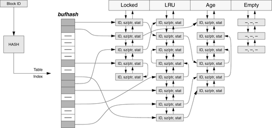
FIGURE 2.18 The buffer cache in 4.3BSD Unix. Cache block lookups based on the block’s ID use the queues anchored in the bufhash array. The array can be sized appropriately to minimize the length of the search queues. Context-based searches use the four queues at the top of the diagram: locked holds important blocks that must not be thrown out (e.g., superblocks); LRU holds blocks in a time-ordered list; age holds blocks that are available for reuse; and empty holds blocks that have had their assigned physical storage stripped from them.
Every block in the cache can be found on exactly two queues. Queues coming in from the left side are hash queues and facilitate quick lookup of a given block, given its Id. Queues coming down from the top are used to determine replacement (a contentmanagement heuristic that will be discussed in more detail in the next chapter) and designate the degree to which a particular block on that list can be replaced without affecting performance. The locked queue holds cache blocks that must not be flushed from the cache (an implementation choice that was later abandoned due to deadlock problems). The LRU queue holds valuable disk blocks in a time-ordered sequence based on last use. The age queue holds blocks of two types: blocks that are not-yet-proven-valuable (i.e., speculatively fetched data) and blocks that have outlived their usefulness and are not expected to be reused any time soon. Items on the age queue are in order of predicted usefulness. The empty queue holds cache blocks that have no available storage left; this is a side effect of having a dynamically determined block size and will be discussed shortly. Cache blocks in this queue are unusable and are waiting for memory space to be freed up.
To find a cached block within the buffer pool, first its identifier is hashed to produce an index into the bufhash array of queue heads. Then the corresponding queue is located and searched, linearly, for the requested cache block. The requested block, once found, is moved to the back of the LRU queue, whether it was on the LRU or age queue to begin with (this is how items are moved from age to LRU when they prove their usefulness by being requested). A block is not moved from one hash queue to another; it is always to be found in the queue identified by the hash product of its identifier (which does not change, because the ID does not change). This represents a clear example of a set-associative organization: each hash queue represents an equivalence class with a dynamically determined cardinality (i.e., some hash queues may contain many cache blocks, while others may be empty; a queue’s contents are determined by the stream of requests serviced by the buffer cache).
To find a suitable block for reuse to hold incoming disk data, the cache is searched from the top queues. The age queue is searched first, as it contains data of questionable usefulness. If it contains a buffer, that buffer is reused for the incoming data. If the age queue is empty, or if it does not contain enough storage to hold the incoming data, the LRU queue is searched next. The cache block at the front of the LRU queue is taken, with it being the least recently used block since all blocks, when used, are put at the back of the queue. As with the cache’s lookup mechanism, this also represents a set-associative organization, one in which different heuristics apply to different sets. The LRU set is managed in a time-ordered manner, and the age set is managed in a completely different manner (e.g., prefetched blocks are put at the back of the queue, newly created empty blocks are put at the front of the queue, and blocks are extracted from the front).
The cache is transparently addressed: the cache is actively searched and not merely indexed; the disk block number, an ID from the backing store, is the key used to search the cache. Because the cache is managed by the same entity that is one of the cache’s clients (i.e., the operating system uses the buffer cache and manages it as well), it is an explicitly managed cache. Thus, this, like the buffer caches in most operating systems, is an example of a software-managed cache.
A Dynamically Defined Cache Block
Even though the preceding discussion called the units of storage within the cache “cache blocks,” BSD’s buffer cache does not hold disk blocks, which are 512 bytes apiece, but rather it holds fragments of files. Because files range significantly in size, and requests to those files also range significantly in size, the buffer cache is designed to accommodate this variability by not using a fixed block size. A block’s size can be as small as the disk block size (512 bytes), or it can range in multiples of 512 B up to 8 KB. At initialization, all buffers are allocated 2 KB of physical space.
If a requested disk block or range of disk blocks is not found in the buffer cache, space is allocated for it by grabbing cache blocks from the age and LRU queues as necessary, and their contents are written back to disk if their status indicates that they are dirty. Assume an example request is for 3 KB of data. If the first acquired block has exactly 3 KB assigned to it, then the process is done. The more interesting scenarios are when this is not the case:
• If the first block acquired has less than 3 KB assigned to it (e.g., say, 2 KB), then a second block is acquired. If the second has less than or is equal to 1 KB, then its storage is added to that of the first, and the second block, now empty of storage, is placed on the empty queue. If the second has more than 1 KB of space, then 1 KB of its storage is added to that of the first block, and the second block is moved to the front of age queue, as it is now available for a new request (its contents having been written back to disk, and it having non-zero space allocated to it).
• If, on the other hand, the first block acquired has more than 3 KB assigned to it, the excess is given to a block on the empty queue, which is then moved to the front of the age queue. If the empty queue holds no blocks, the excess storage remains attached to the block in question and is just wasted until that block is reclaimed for another use.
One way to look at this is that the cache supports a single, atomic cache block size of 512 B, but the fundamental cache organization and operation are centered around a logical block size that is dynamically determined on a request-by-request basis, with a logical block being assembled dynamically from an integral number of atomic blocks.
2.6.3 Another Dynamic Cache Block: Trace Caches
A similar example to the dynamic cache block of BSD’s buffer cache is the familiar trace cache, a solidstate cache that implements a dynamically assembled cache block. The cache block contents can represent several non-contiguous streams of bytes in the backing store. While the BSD buffer cache changes the cache’s block size to match each incoming request’s size but takes its data from a single stream of bytes from the backing store, the trace cache dynamically redefines not only the block size, but the block contents as well. On a block-by-block basis, the trace cache assembles into a single block (which holds a contiguous array of instructions) data from up to three disjoint locations, i.e., past one or more branches.
The trace cache mechanism directly addresses the problem of providing high-bandwidth instruction-fetch. The issues in instruction-fetch today include the following:
• Basic blocks are small, and conditional branches are frequent.
• To match issue and execute bandwidths, the required bandwidths of instruction-fetch are high, and to match these one must successfully predict multiple branches in a single cycle.
• Assuming one can predict multiple branches per cycle, multiple corresponding fetch addresses must be produced. Instructions from more than one cache block must be fetched in a single clock cycle, and these disjoint instruction streams (each of which may comprise a full cache block or a partial cache block) must be rearranged and reassembled into the desired execution order.
The trace cache addresses these issues by placing into a single cache block instructions from different basic blocks: the control-flow path has been predicted, so each cache block represents a trace [Fisher 1981] through the control-flow graph. This addresses the issues above by placing multiple basic blocks into a single fetch unit, obviating any need for fetching multiple cache blocks or rearranging fetched instructions.
The trace cache mechanism is particularly interesting because it represents a dynamic redefinition of the cache block itself. Remember that a cache block is generally considered to be a set of data items that are contiguous in the backing store and therefore make up a convenient unit to fetch from the backing store—the convenience is from the point of view of the mechanism responsible for fetching data from the backing store (the memory and/or cache controller). The trace cache completely redefines the concept of a cache block: by dynamically assembling together the instructions that a processor core needs (as opposed to a collection of items that a compiler placed together), this turns the cache-resident block into a convenient unit of instruction-fetch from the processor core’s point of view. The mechanism really strides the line between an unorthodox cache organization and a hybrid of cache organization and content-management heuristic. Allowing a cache block to contain instructions from disjoint streams (i.e., past branches) is an interesting twist on cache organization. Dynamically assembling the cache blocks is a form of content-management heuristic.
The following sections describe the various forms of trace cache that have been proposed and built (e.g., fetch mechanisms in ELI and ROPE, tree-VLIW structures, the fill unit, the shadow cache, the dynamic flow instruction cache, and the trace cache) plus a few additional studies that help put its development into historical perspective. The two primary concepts embodied in the trace cache—a cache block holding disjoint streams and its dynamic assembly—both find their roots in the late 1970s and 1980s. Briefly, the history discussed goes as follows:
• Early research in very long instruction word (VLIW) architecture identifies the instruction-fetch problem (1980).
• Several architectures (ELI, ROPE) provide support for multiple simultaneous branch instructions and simultaneous instruction-fetch from non-contiguous streams (1980–1985).
• Tree-VLIW puts non-contiguous instruction streams into the same cache block (1987).
• The fill unit dynamically assembles a cache block from a sequential stream, reordering instructions as necessary (1988).
• Multiple branches are predicted in a single cycle (1993).
• The shadow cache dynamically assembles a cache block, combining instructions from non-contiguous streams (1994).
• Called the dynamic flow instruction cache, the trace cache is patented by Peleg and Weiser (1995).
• A significant range of instruction-fetch solutions is explored, underscoring the difficulty of fetching non-contiguous streams (1995).
• The trace cache appears, which dynamically combines instructions past two branches (i.e., from three non-contiguous streams), using a generic cache block structure (1996).
VLIW and the Instruction-Fetch Problem
The problem of providing enough fetch bandwidth to feed the execution units is not new. Early research in VLIW architectures (also called horizontal microcode) identified this as a primary performance-limiting issue, citing explicitly the density of branches, the need to operate on multiple potentially non-contiguous streams, and the requirement of performing (which would today be predicting) multiple conditional branches simultaneously:
The designs of all very wide microengines we have seen to date have what we consider to be a serious defect: in essence, only one test [i.e., conditional branch] instruction may be scheduled per wide instruction…. Thus no matter how many FU’s and data paths are thrown at the algorithm, a serious bottleneck will occur while awaiting the tests to be resolved one at a time. [Fisher 1980, p. 65]
Since the instructions within a basic block usually have serial dependencies, code rearrangement has to range over several basic blocks. In horizontal microcode, several data path operations can often be started simultaneously. Unless several conditional jumps are evaluated at once, the ratio of jumps to straight-line code becomes unacceptably high. Furthermore, the density of conditional jumps foils the effectiveness of the traditional pre-fetch mechanism in which the next instruction is pre-fetched sequentially. [Karplus & Nicolau 1985, p. 12]
To combat the problem, researchers developed sophisticated scheduling and instruction-packing techniques to ensure that a constant stream of multiple instructions per cycle was being fed to the back-end processor core, designed to work hand-in-hand with the compiler and supporting scheduling software (e.g., Fisher [1980, 1981, 1983], Fisher et al. [1984], Karplus and Nicolau [1985], Ebcioglu [1987, 1988], Aiken and Nicolau [1988]). Two schemes that resemble the modern trace cache are the ELI and ROPE mechanisms, both of which implement multi-way branches and fetch instructions from logically non-contiguous code locations. ELI is an explicit VLIW architecture; ROPE is a general instruction-fetch mechanism explicitly targeted for both VLIW and serial (RISC and/or CISC) processing architectures.
Multi-way Branches and Disjoint I-Fetch in ELI and ROPE.
Fisher puts the problem well, an argument that is still applicable to the architectures of today:
Comparing VLIWs with vector machines illustrates the problems to be solved. VLIWs put fine-grained, tightly coupled, but logically unrelated operations in single instructions. Vector machines do many fine-grained, tightly coupled, logically related operations at once to the elements of a vector. Vector machines can do many parallel operations between tests; VLIWs cannot. Vector machines can structure memory references to entire arrays or slices of arrays; VLIWs cannot. We’ve argued, of course, that vector machines fail on general scientific code for other reasons. How do we get their virtues without their vices?
VLIWs need clever jump mechanisms.
Short basic blocks impl[y] a lack of local parallelism. They also imply a low ratio of operations to tests. If we are going to pack a great many operations into each cycle, we had better be prepared to make more than one test per cycle. [Fisher 1983, pp. 145–146]
ELI: Extremely Long Instructions.
The solution of the day was to perform multi-way branches, and ELI’s mechanism differed from previous schemes in that it performed independent branches simultaneously: ELI put multiple conditional branches into the same VLIW instruction and executed them simultaneously [Fisher 1980, 1983].
However, performing a multi-way branch implies that, to avoid stalling, all of the possible target instruction streams must be prefetched simultaneously. The solution offered in ELI, pictured in Figure 2.19, is a multi-banked instruction memory, interleaved to the same degree as the degree of multi-branching, with the instruction streams at the various target code blocks mapped to the same offset in different banks. All n banks are accessed simultaneously with the same index (effectively representing a single, logical cache block), yielding n target instruction streams, one of which is ultimately selected by the branchresolution hardware.

FIGURE 2.19 Instruction-fetch in Fisher’s ELI architecture. This illustrates the mechanism for resolving an n-way branch instruction, which has 2n possible branch targets; all targets point to independent instruction streams housed in the same VLIW instruction. At the bottom of the figure is the code that the microinstruction arrangement would implement. Later implementations of ELI simplified this branch architecture to support a linear if-then-else chain called a vine, pictured at the bottom.
ROPE: Ring Of Prefetch Elements
Karplus and Nicolau [1985] use a similar multi-banked scheme to implement a general high-bandwidth fetch engine called ROPE, illustrated in Figure 2.20. ROPE is targeted at supporting any back-end processor architecture that requires high instruction-fetch bandwidth, whether VLIW or serial RISC/CISC. Like ELI, ROPE executes a multi-way branch and fetches simultaneously out of multiple banks to avoid stalling. The primary difference between ROPE and the fetch engine in ELI is that the banks in ROPE are not slaved to one another as they are in ELI; ROPE’s prefetch engines operate independently, each passing a follow-on target address to the next element in the ring. Thus, each element can be fetching simultaneously, producing at the output of the fetch unit a large number of non-contiguous instruction streams.
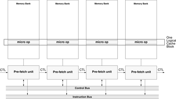
Tree-VLIW Instructions
ELI can be said to support a logical cache block made up of multiple, logically non-contiguous instruction streams. However, the instruction streams are, in fact, contiguous in terms of physical addresses. A fair amount of compiler and hardware support packs these logically non-contiguous instructions together into the same physical instruction word to support the multi-way branch.
A similar mechanism that moves closer to the trace cache concept (i.e., the idea of allowing a cache block to contain atomic instructions that span a break in sequential control flow) is the tree-VLIW instruction word, described by Ebcioglu in 1987 and 1988, but not named so until later. The basic premise of the architecture is that, unlike the previous VLIW architectures that support multiple exit points out of an instruction word in which every atomic instruction is executed, this architecture supports conditional execution of the atomic instructions within the long instruction word. This is illustrated in Figure 2.21. The DAG represents a single instruction, 500–1800 bits wide, in which multiple paths of control exist. Only those atomic instructions on the taken control path are executed. Because the instruction word contains multiple paths of control, it defines a cache design that explicitly holds multiple disjoint instruction streams, each potentially fairly long, given even the smallest targeted word size (500 bits). Note that the structure of this multi-branch operation is an n = 2 organization of Fisher’s vine structure [Fisher 1983].
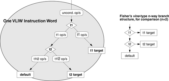
FIGURE 2.21 Ebcioglu’s tree-like instruction word. On each edge of the control-flow graph (which represents a single VLIW instruction), multiple conditional operations can be placed. These are only conditional upon being on the dynamically executed path through the control-flow graph. The figure illustrates this, showing the logic value of tests 1 and 2 that is required for each operation or set of operations to be performed: e.g., “tl![]() op/s” means 0 or more operations that will be executed if, when the block is executed, t1 dynamically evaluates to true and t2 dynamically evaluates to false.
op/s” means 0 or more operations that will be executed if, when the block is executed, t1 dynamically evaluates to true and t2 dynamically evaluates to false.
The Fill Unit
The idea of dynamically assembling a cache block’s contents originates with Melvin’s fill unit [Melvin et al. 1988], which dynamically reorders and repacks fetched microoperations (e.g., RISC-like instructions) into the decoded instruction cache’s blocks, taking its instructions from either a non-decoded instruction cache or main memory. In cooperation with the prefetch buffer, microoperation generator, address re-alias unit, and decoded instruction cache (see Figure 2.22), the fill unit interprets incoming instructions, reorders them, renames their register operands, and reformats them to use the format that the back-end processing core expects, which may differ significantly from the compiler’s target. The fill unit dynamically redefines the instruction stream, checks inter-instruction dependences, and only finalizes a group of instructions (stops filling an i-cache block, thus defining the boundaries of instruction-fetch) when a branch is detected or the capacity of the i-cache block is exceeded. The combined portions of the design, shown highlighted by the grey blob in the figure, are very similar to the modern trace cache, with the significant difference being that the design does not attempt to create long sequences of instructions that span a change in control flow.
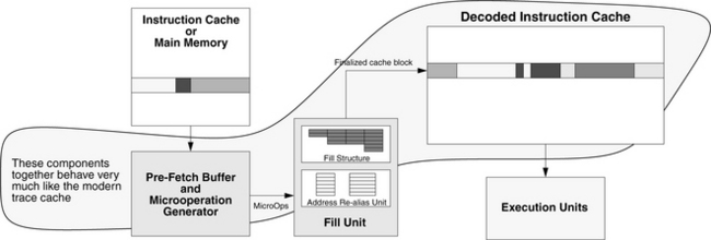
Multi-Branch Predictor and Branch-Address Cache
As Fisher points out [1983], VLIWs need clever jump mechanisms, and the observation extends to any scalar architecture that executes multiple instructions simultaneously. Modern architectures do not typically use the multi-way branch instructions and architectures of the 1980s, largely due to the development of accurate branch prediction (i.e., the two-level adaptive training branch predictor [sic][Yeh & Patt 1991], a hybrid of Jim Smith’s dynamic predictors [1981b], which introduced adaptive state machines such as a table of n-bit saturating up/down counters, and prediction based on branch history, the mechanism described by Lee and Smith [1984] and represented as static training by Yeh & Patt, which introduced the two-level approach of using a per-branch n-bit history of outcomes as an index). Successful prediction of single two-way branches supports the same degree of instruction-fetch bandwidth available in the 1980s with multi-way branches. However, even this is insufficient for architectures of the mid-1990s, which require more than just two basic blocks of instructions per cycle.
To increase the visible window of instructions to fetch, Yeh presents a branch predictor design that predicts two branches per cycle and a branch-address cache that provides multiple target addresses per cycle [Yeh et al. 1993]. Coupled with these mechanisms is an instruction cache reminiscent of ELI and ROPE: a highly banked, pseudo-multi-ported cache that can produce multiple (four) non-contiguous cache blocks per cycle. The multiple-branch-predictor-cum-branch-address-cache mechanism is similar to the trace cache in its goal of delivering a stream of instructions that are potentially non-contiguous in memory. Like Melvin’s fill unit, the mechanism does not put into a single cache block, either physical or logical, sequences of instructions that span a change in control flow.
The Shadow Cache
In this regard—to wit, dynamically creating cache blocks filled with instructions that are non-contiguous in the memory space and that represent multiple streams of instructions that lie on different sides of a control-flow decision—Franklin and Smotherman [1994] present the first real trace cache, called the shadow cache. Using a modified fill unit (see Figure 2.23), the shadow cache dynamically assembles shadow cache blocks from disjoint regions in the code space. The shadow cache is operated in parallel with the instruction cache and is filled from the instruction cache (like both Melvin’s fill unit and Rotenberg’s trace cache). The design creates a linear array of instructions that can extend past (at most) one branch. The scheme does not lend itself well to an extension of handling arbitrary numbers of branches, because, at least in the experimental implementation evaluated in the paper, the shadow cache’s block holds instructions from both taken and non-taken paths past the branch.

One of the disadvantages of dynamically defining the cache block in this way is that two different paths dynamically taken through a basic block (e.g., two vectors into a basic block) can produce two different cache blocks, thereby effectively lowering the cache’s capacity due to the cache holding replicated instructions. This is not specific to the shadow cache; it is generally true of the trace cache concept, a function of dynamically assembling a multi-instruction trace.
The shadow cache implementation represents an execution architecture that lies somewhere between out-of-order superscalar and VLIW. One of the goals of the work is to provide the implementation simplicity of VLIW with the programming and compiler-target simplicity of a sequential architecture. To this end, the shadow cache maintains a block structure that is targeted for a specific back-end implementation, and its fill unit does a modicum of rearranging instructions to match the back-end execution hardware’s expectations. Compared to a modern trace cache, the shadow cache holds instructions in issued order rather than fetched order. It is more or less a de facto VLIW backend, with the fill unit and shadow cache effectively hiding implementation details from the program and compiler.
A Range of Fetch and Align Strategies
Conte explores a wide range of instruction-fetch implementations using a traditional cache design, focusing on the mask-and-reorder circuitry that is required to handle non-contiguous streams of instructions that span more than one basic block [Conte et al. 1995]. The study explores schemes that range from lower bound (fetch a single cache block and extract instructions, stopping at first branch) to upper bound (fetch enough instructions from as many cache blocks as required to fill the fetch buffer) and includes the following:
• Interleaved sequential: fetch two cache blocks, sequentially ordered, and stop filling buffer at first branch
• Banked sequential: fetch two cache blocks, the second based on branch target buffer output (i.e., not necessarily sequential blocks, and so the scheme effectively handles inter-block branches), and stop filling buffer on first intra-block branch
• Collapsing buffer: fetch two cache blocks, the second based on branch target buffer output (i.e., not necessarily sequential blocks, and so the scheme effectively handles inter-block branches), and handle intra-block branches by “collapsing” the buffer (i.e., masking out jumped-over instructions and compacting the remainder)
The experimental results show that, as complexity is added to the fetch design, the various schemes improve upon the lower bound and approach the performance of the upper bound, but one of the most important contributions is to demonstrate just how much work is involved in handling non-contiguous instruction streams and how expensive it can be in both cases of branches jumping to instructions within the same cache block and branches jumping to instructions in different cache blocks.
The Patented Design
This brings us to Peleg and Weiser’s dynamic flow instruction cache, a mechanism that solves the problem of mask and reorder (among other issues) by keeping the masked-and-reordered instruction stream in the cache. Peleg, a student at Technion in Israel, and Weiser of Intel, also an adjunct professor at Technion and Peleg’s advisor, patented their invention in 1995 [Peleg & Weiser 1995], shown in Figure 2.24. This patent forms the basis of Intel’s commercialized trace cache. The motivation of the design:
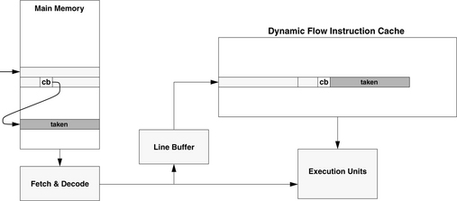
With prior art instruction cache memories, when a branch is taken, the next requested instruction may be on another line. Therefore, some of the instructions stored in the cache memory may never be used and moreover, the organization on each line is independent of branching. In contrast, with the present invention, the organization of the cache memory is dynamically built on the order of execution of the instructions. [Peleg & Weiser 1995]
The main contribution of the design is that the data layout stored in the cache is more generic than previous designs. Melvin’s fill unit and Franklin’s shadow cache both tie the cache block structure to the back-end processing core’s implementation, whereas Peleg’s design puts no such restriction on the cache block format. Though the patent description above suggests that the instruction ordering represents instruction execution (which would imply an invention similar to the fill unit and shadow cache), the instruction stream is only reordered at the basicblock level: a cache block can hold up to two non-contiguous basic blocks, and instructions within each basic block are stored in the cache in program order.
The mechanism trades off space for instruction-fetch bandwidth: at any given moment, the cache contains potentially significant excess or unused space (e.g., 32 bytes per block, all of which may or may not be filled). In addition, like the fill unit and shadow cache, the dynamic flow cache suffers the overhead of storing a given static instruction multiple times at multiple locations in the cache (every basic block is considered to be a follow-on from the previous basic block, as well as the beginning of a new trace). The bandwidth is achieved by eliminating the need to predict multiple cache blocks for fetch (the predictions are implicit in the trace stored within a block) and eliminating the need to mask and reorder a stream of fetched instructions that span multiple basic blocks (such alignment is implicit in the instruction stream stored within a block).
The “Trace Cache”
Rotenberg’s trace cache extends the number of basic blocks represented in a single cache block, something very important given the amount of attention paid to predicting more than one branch in a single cycle. The authors describe the problem well:
The job of the fetch unit is to feed the dynamic instruction stream to the decoder. A problem is that instructions are placed in the cache in their compiled order. Storing programs in static form favors fetching code that does not branch or code with large basic blocks. Neither of these cases is typical of integer code. [Rotenberg et al. 1996, p. 25]
The trace cache extends Franklin and Smotherman’s shadow cache and Peleg’s design to handle non-contiguous streams spanning two branches (i.e., up to three basic blocks), and it does so in a generic and scalable manner that would support even more basic blocks. Like Peleg’s design, the trace cache stores instructions in program order within a basic block, as opposed to storing reordered instructions. The cache has a fixed maximum block size of 16 instructions and fills this block from the dynamic instruction-execution stream (i.e., from disjoint regions in the code space), up to 16 instructions or a third conditional branch, whichever comes first (see Figure 2.25). Like the dynamic flow cache, the trace cache trades off storage for bandwidth; a cache block may or may not be completely filled, and a given instruction may reside in multiple locations within the cache, corresponding to multiple traces.
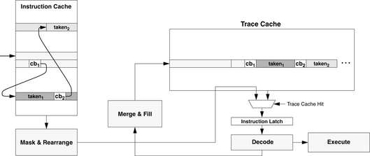
Note that the sets of the cache maintain a nonexclusive relationship with each other, if a given instruction can be found within multiple cache blocks (this is potentially true of the fill unit, shadow cache, and dynamic flow cache as well). This is not considered a problem because most operating systems treat the code space as a non-writable region. Note, however, that some “operating systems” are, in fact, just program loaders and do not enforce or guarantee this form of resource management and protection.
In a similar vein, the trace cache, like the fill unit and shadow cache, maintains a non-inclusive relationship with the traditional instruction cache with which it operates in parallel. A given static instruction can be found in both caches, but it need not be. This is not considered a problem because most operating systems treat the code space as a non-writable region.
1An aside: one could attempt to pull apart the use of tags and the choice of transparent or non-transparent addressing, giving eight different types instead of four. For example, one could in theory build a transparently addressed scratchpad in which the cache contents are explicitly managed by the application software. The cache has no tag store, but the addressing scheme is transparent. This could be done, for example, if an address translation step was performed before cache index, such as inserting a TLB before indexing an SRAm. However, the TLB in this scheme would become a de facto tags array, yielding a software-managed cache.
2Portions reprinted, with permission, from “Uniprocessor virtual memory without TLBs,” by B. Jacob and T. Mudge. IEEE Transactions on Computers, 50(5), 482–499, May 2001. Copyright © 2001 IEEE.
3Note that the SunOS scheme only solves the problem for direct-mapped virtual caches or set-associative virtual caches with physical tags. Shared data can still exist in two different blocks of the same set in an associative, virtually indexed, virtually tagged cache.