
Worked Example 2
Pumping Installation
Chapter Outline
Design and Construction Philosophy
1. 3-tonne vessel arrives on-site complete with nozzles and manhole doors in place.
2. Pipe gantry and vessel support steel arrive piece small.
3. Pumps, motors, and bedplates arrive as separate units.
4. Stairs arrive in sections with treads fitted to a pair of stringers.
5. Suction and discharge headers are partially fabricated with weldolet tees in place. Slip-on flanges to be welded on-site for valves, vessel connection, and blanked-off ends.
6. Suction and discharge lines from pumps to have slip-on flanges welded on-site after trimming to length.
7. Drive, couplings to be fitted before fitting of pipes to pumps, but not aligned.
8. Hydro test to be carried out in one stage. Hydro pump connection at discharge header end. Vent at top of vessel. Pumps have drain points.
9. Resource restraints require Sections A and B of suction and discharge headers to be erected in series.
10. Suction to pumps is prefabricated on-site from slip-on flange at valve to field weld at high-level bend.
11. Discharge from pumps is prefabricated on-site from slip-on flange at valve to field weld on high-level horizontal run.
12. Final motor coupling alignment to be carried out after hydro test in case pipes have to be re-welded and aligned after test.
In this example it is necessary to produce a material take-off from the layout drawings so that the erection manhours can be calculated. The manhours can then be translated into man days and, by assessing the number of men required per activity, into activity durations. The manhour assessment is, of course, made in the conventional manner by multiplying the operational units, such as numbers of welds or tonnes of steel, by the manhour norms used by the construction organization. In this exercise the norms used are those published by the OCPCA (Oil & Chemical Plant Contractors Association). These are base norms that may or may not be factorized to take account of market, environmental, geographical, or political conditions of the area in which the work is carried out. It is obvious that the rate for erecting a tonne of steel in the UK is different from erecting it in the wilds of Alaska.
The sequence of operations for producing a network programme and EVA analysis is as follows:
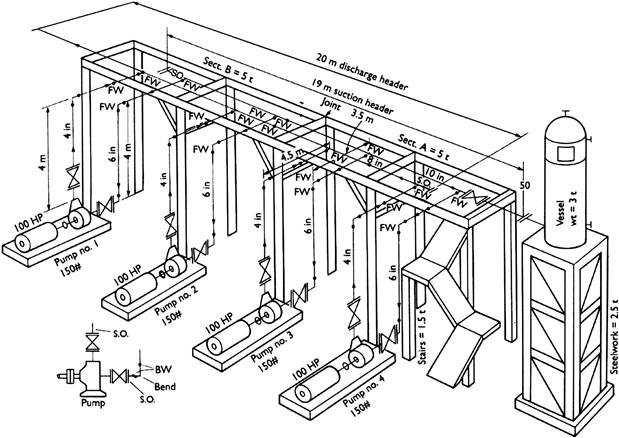
1. Study layout drawing or piping isometric drawings (Figure 48.1).
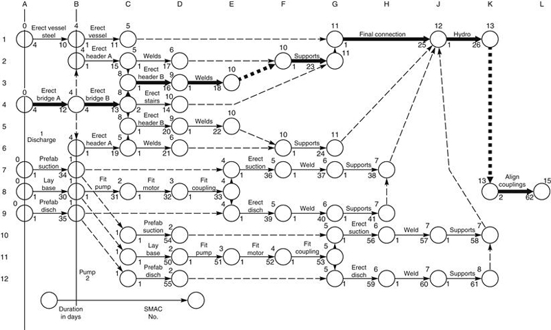
2. Draw a construction network. Note that at this stage it is only possible to draw the logic sequences (Figure 48.2) and allocate activity numbers.
3. From the layout drawing, prepare a take-off of all the erection elements such as number of welds, number of flanges, weight of steel, number of pumps, etc.
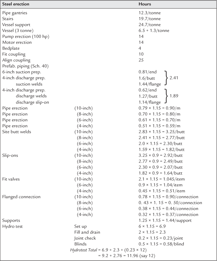
4. Tabulate these quantities on an estimate sheet (Figure 48.3) and multiply these by the OCPCA norms given in Table 48.1 to give the manhours per operation.
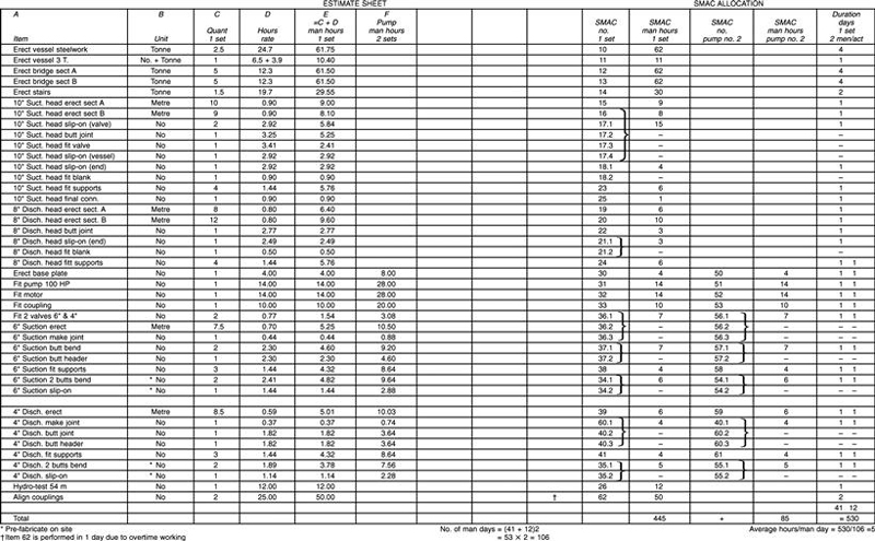
Figure 48.3
5. Decide which operations are required to make up an activity on a network and list these in a table. This enables the manhours per activity to be obtained.
6. Assess the number of men required to perform any activity. By dividing the activity manhours by the number of men the actual working hours and consequently working days (durations) can be calculated.
7. Enter these durations in the network programme.
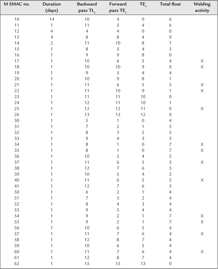
8. Carry out the network analysis, giving floats and the critical path (Table 48.2).
9. Draw up the EVA analysis sheet (Table 48.3) listing activities, activity (SMAC) numbers, and durations.
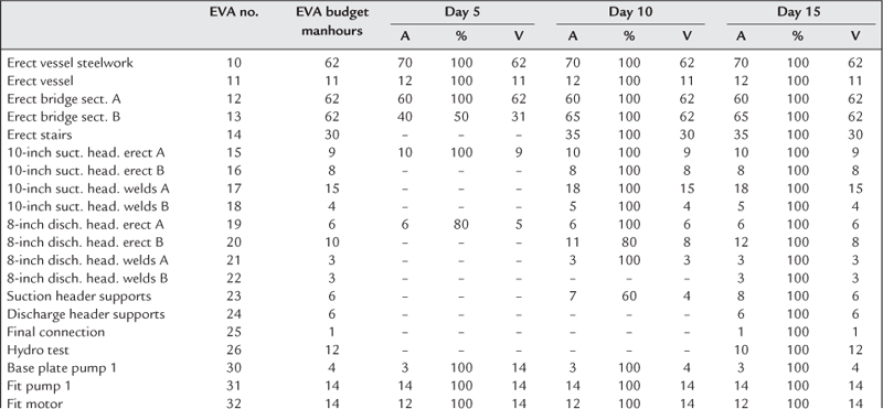

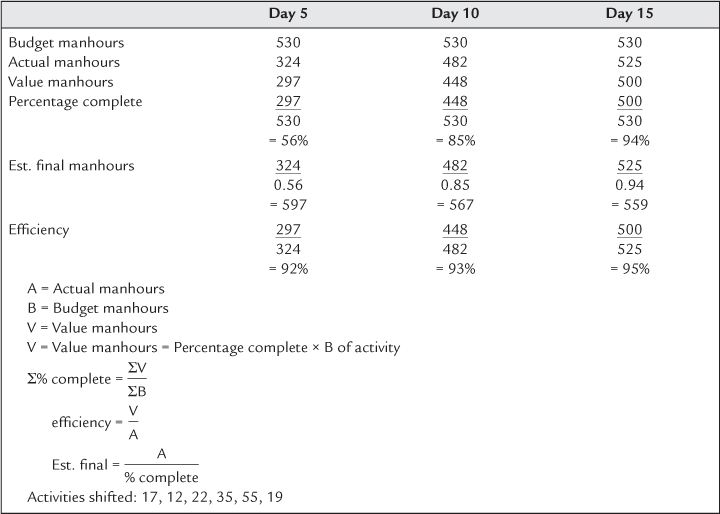
10. Carry out EVA analysis at weekly intervals. The basis calculations for value hours, efficiency, etc., are shown in Table 48.4.
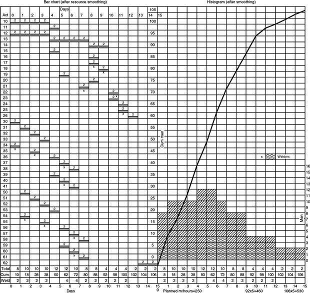
11. Draw a bar chart using the network as a basis for start and finish of activities (Figure 48.4).

12. Place the number of men per week against the activities on the bar chart.
13. Add up vertically per week and draw the labour histogram and ‘S’ curve.
14. Carry out a resource-smoothing exercise to ensure that labour demand does not exceed supply for any particular trade. In any case, high peaks or troughs are signs of inefficient working and should be avoided here (Figure 48.5). (Note: This smoothing operation only takes place with activities which have float.)
15. Draw the project control curves using the weekly EVA analysis results to show graphically the relationship between:
• Predicted final hours (Figure 48.6)

16. Draw control curves showing:
• Percentage complete (progress)
• Efficiency (Figure 48.6)
The procedures outlined above will give a complete control system for time and cost for the project as far as site work is concerned.
Cash Flow
Cash flow charts show the difference between expenditure (cash outflow) and income (cash inflow). Since money is the common unit of measurement, all contract components such as manhours, materials, overheads, and consumables have to be stated in terms of money values.
It is convenient to set down the parameters that govern the cash flow calculations before calculating the actual amounts. For the example being considered:
1. There are 1748 productive hours in a year (39 hours/week × 52) – 280 days of annual holidays, statutory holidays, sickness, and travelling allowance and induction.
2. Each manhour costs, on average, ≤5 in actual wages.
3. After adding payments for productivity, holiday credits, statutory holidays, course attendance, radius, and travel allowance, the taxable rate becomes ≤8.40/hour.
4. The addition of other substantive items such as levies, insurance, protective clothing and non-taxable fares, and lodging increases the rate by ≤2.04 to ≤10.44/hour.
| Consumables | 5% |
| Overheads | 10% |
| Profit | 5% |
| Total | 20% |
7. The total charge-out rate is, therefore, 10.44 × 1.2 = ≤12.53 per hour.
8. In this particular example:
(a) the men are paid at the end of each day at a rate of ≤8.40/hour.
(b) the other substantive items of ≤2.04/hour are paid weekly.
(c) income is received weekly at the charge-out rate of ≤12.53/hour.
To enable the financing costs to be calculated at the estimate stage, cash flow charts are usually only drawn to show the difference between planned outgoings and planned income.
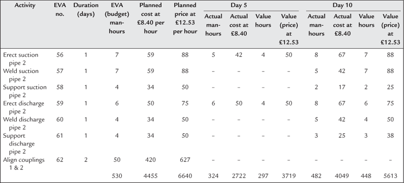
However, once the contract is under way a constant check must be made between actual costs (outgoings taken from time cards) and valued income derived from valuations of useful work done. The calculations for days 5 and 10 in Table 48.5 show how this is carried out. When these figures are plotted on a chart as in Figure 48.7 it can be seen that for
| days 0–5 | the cash flow is negative (i.e., outgoings exceed income). |
| days 5–8 | the cash flow is positive. |
| days 8–10 | the cash flow is negative. |
| days 10–15 | the cash flow is positive. |
| On day 15, | the total value is recovered assuming there are no retentions. |


The planned costs of the other substantives can be calculated for each period by multiplying the planned cumulative outgoings by the ratio of 0.243.
| For day 5 | the substantive costs are 2391 × 0.243 = ≤581. |
| For day 10 | the substantive costs are 3826 × 0.243 = ≤930. |
| For day 15 | the substantive costs are 4455 × 0.243 = ≤1083. |
These costs are plotted on the chart and, when added to the planned labour costs, give total planned outgoings of:
≤2391 + 581 = 2972 for day 5.
≤3826 + 930 = 4756 for day 10.
≤4455 + 1083 = 5538 for day 15.
To obtain the actual total outgoings it is necessary to multiply the actual labour costs by 1.243: e.g., for day 5, the actual outgoings will be
2722 × 1.243 = ≤3383
and for day 10 they will be
4049 × 1.243 = ≤5033.
The total planned and actuals can therefore be compared on a regular basis.