Certain Python objects have attributes, data values or executable code such as methods, associated with them. Attributes are accessed in the dotted attribute notation, which includes the name of the associated object, and were introduced in the Core Note in Section 2.14. The most familiar attributes are functions and methods, but some Python types have data attributes associated with them. Objects with data attributes include (but are not limited to): classes, class instances, modules, complex numbers, and files.

It may seem unusual to regard types themselves as objects since we are attempting to just describe all of Python’s types to you in this chapter. However, if you keep in mind that an object’s set of inherent behaviors and characteristics (such as supported operators and built-in methods) must be defined somewhere, an object’s type is a logical place for this information. The amount of information necessary to describe a type cannot fit into a single string; therefore types cannot simply be strings, nor should this information be stored with the data, so we are back to types as objects.

We will formally introduce the type() BIF below, but for now, we want to let you know that you can find out the type of an object by calling type() with that object:

Let us look at this example more carefully. It does not look tricky by any means, but examine the return value of the call. We get the seemingly innocent output of <type ‘int’>, but what you need to realize is that this is not just a simple string telling you that 42 is an integer. What you see as <type ‘int’> is actually a type object. It just so happens that the string representation chosen by its implementors has a string inside it to let you know that it is an int type object.

Now you may ask yourself, so then what is the type of any type object? Well, let us find out:

Yes, the type of all type objects is type. The type type object is also the mother of all types and is the default metaclass for all standard Python classes. It is perfectly fine if you do not understand this now. This will make sense as we learn more about classes and types.

With the unification of types and classes in Python 2.2, type objects are playing a more significant role in both object-oriented programming as well as day-to-day object usage. Classes are now types, and instances are now objects of their respective types.

Python has a special type known as the Null object or NoneType. It has only one value, None. The type of None is NoneType. It does not have any operators or BIFs. If you are familiar with C, the closest analogy to the None type is void, while the None value is similar to the C value of NULL. (Other similar objects and values include Perl’s undef and Java’s void type and null value.) None has no (useful) attributes and always evaluates to having a Boolean False value.

Core Note: Boolean values

All standard type objects can be tested for truth value and compared to objects of the same type. Objects have inherent True or False values. Objects take a False value when they are empty, any numeric representation of zero, or the Null object None.

The following are defined as having false values in Python:

• None

• False (Boolean)

• Any numeric zero:

• 0 (integer)

• 0.0 (float)

• 0L (long integer)

• 0.0+0.0j (complex)

• ““ (empty string)

• [] (empty list)

• () (empty tuple)

• {} (empty dictionary)

Any value for an object other than those above is considered to have a true value, i.e., non-empty, non-zero, etc. User-created class instances have a false value when their nonzero (__nonzero__()) or length (__len__()) special methods, if defined, return a zero value.

Code objects are executable pieces of Python source that are byte-compiled, usually as return values from calling the compile() BIF. Such objects are appropriate for execution by either exec or by the eval() BIF. All this will be discussed in greater detail in Chapter 14.

Code objects themselves do not contain any information regarding their execution environment, but they are at the heart of every user-defined function, all of which do contain some execution context. (The actual byte-compiled code as a code object is one attribute belonging to a function.) Along with the code object, a function’s attributes also consist of the administrative support that a function requires, including its name, documentation string, default arguments, and global namespace.

These are objects representing execution stack frames in Python. Frame objects contain all the information the Python interpreter needs to know during a runtime execution environment. Some of its attributes include a link to the previous stack frame, the code object (see above) that is being executed, dictionaries for the local and global namespaces, and the current instruction. Each function call results in a new frame object, and for each frame object, a C stack frame is created as well. One place where you can access a frame object is in a traceback object (see the following section).

When you make an error in Python, an exception is raised. If exceptions are not caught or “handled,” the interpreter exits with some diagnostic information similar to the output shown below:

The traceback object is just a data item that holds the stack trace information for an exception and is created when an exception occurs. If a handler is provided for an exception, this handler is given access to the traceback object.

Slice objects are created using the Python extended slice syntax. This extended syntax allows for different types of indexing. These various types of indexing include stride indexing, multi-dimensional indexing, and indexing using the Ellipsis type. The syntax for multi-dimensional indexing is sequence[start1 : end1, start2 : end2], or using the ellipsis, sequence [..., start1 : end1]. Slice objects can also be generated by the slice() BIF.

Stride indexing for sequence types allows for a third slice element that allows for “step”-like access with a syntax of sequence[starting_index : ending_index : stride].

Support for the stride element of the extended slice syntax have been in Python for a long time, but until 2.3 was only available via the C API or Jython (and previously JPython). Here is an example of stride indexing:

Ellipsis objects are used in extended slice notations as demonstrated above. These objects are used to represent the actual ellipses in the slice syntax (...). Like the Null object None, ellipsis objects also have a single name, Ellipsis, and have a Boolean True value at all times.

XRange objects are created by the BIF xrange(), a sibling of the range() BIF, and used when memory is limited and when range() generates an unusually large data set. You can find out more about range() and xrange() in Chapter 8.

For an interesting side adventure into Python types, we invite the reader to take a look at the types module in the standard Python library.

Comparison operators are used to determine equality of two data values between members of the same type. These comparison operators are supported for all built-in types. Comparisons yield Boolean True or False values, based on the validity of the comparison expression. (If you are using Python prior to 2.3 when the Boolean type was introduced, you will see integer values 1 for True and 0 for False.) A list of Python’s value comparison operators is given in Table 4.1.

Table 4.1. Standard Type Value Comparison Operators

Note that comparisons performed are those that are appropriate for each data type. In other words, numeric types will be compared according to numeric value in sign and magnitude, strings will compare lexicographically, etc.

Also, unlike many other languages, multiple comparisons can be made on the same line, evaluated in left-to-right order:

We would like to note here that comparisons are strictly between object values, meaning that the comparisons are between the data values and not the actual data objects themselves. For the latter, we will defer to the object identity comparison operators described next.

In addition to value comparisons, Python also supports the notion of directly comparing objects themselves. Objects can be assigned to other variables (by reference). Because each variable points to the same (shared) data object, any change effected through one variable will change the object and hence be reflected through all references to the same object.

In order to understand this, you will have to think of variables as linking to objects now and be less concerned with the values themselves. Let us take a look at three examples.

Example 1: foo1 and foo2 reference the same object

When you look at this statement from the value point of view, it appears that you are performing a multiple assignment and assigning the numeric value of 4.3 to both the foo1 and foo2 variables. This is true to a certain degree, but upon lifting the covers, you will find that a numeric object with the contents or value of 4.3 has been created. Then that object’s reference is assigned to both foo1 and foo2, resulting in both foo1 and foo2 aliased to the same object. Figure 4-1 shows an object with two references.

Figure 4-1. foo1 and foo2 reference the same object

Example 2: foo1 and foo2 reference the same object

This example is very much like the first: A numeric object with value 4.3 is created, then assigned to one variable. When foo2 = foo1 occurs, foo2 is directed to the same object as foo1 since Python deals with objects by passing references. foo2 then becomes a new and additional reference for the original value. So both foo1 and foo2 now point to the same object. The same figure above applies here as well.

Example 3: foo1 and foo2 reference different objects

This example is different. First, a numeric object is created, then assigned to foo1. Then a second numeric object is created, and this time assigned to foo2. Although both objects are storing the exact same value, there are indeed two distinct objects in the system, with foo1 pointing to the first, and foo2 being a reference to the second. Figure 4-2 shows we now have two distinct objects even though both objects have the same value.

Figure 4-2. foo1 and foo2 reference different objects

Why did we choose to use boxes in our diagrams? Well, a good way to visualize this concept is to imagine a box (with contents inside) as an object. When a variable is assigned an object, that creates a “label” to stick on the box, indicating a reference has been made. Each time a new reference to the same object is made, another sticker is put on the box. When references are abandoned, then a label is removed. A box can be “recycled” only when all the labels have been peeled off the box. How does the system keep track of how many labels are on a box?

Each object has associated with it a counter that tracks the total number of references that exist to that object. This number simply indicates how many variables are “pointing to” any particular object. This is the reference count that we introduced in Chapter 3, Section 3.5.4. Python provides the is and is not operators to test if a pair of variables do indeed refer to the same object. Performing a check such as

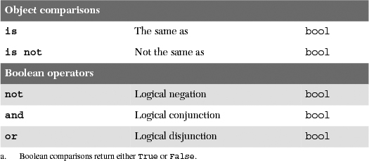
The object identity comparison operators all share the same precedence level and are presented in Table 4.2.

Table 4.2. Standard Type Object Identity Comparison Operators

In the example below, we create a variable, then another that points to the same object.

Both the is and not identifiers are Python keywords.

Core Note: Interning

In the above examples with the foo1 and foo2 objects, you will notice that we use floating point values rather than integers. The reason for this is although integers and strings are immutable objects, Python sometimes caches them to be more efficient. This would have caused the examples to appear that Python is not creating a new object when it should have. For example:

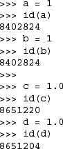
In the above example, a and b reference the same integer object, but c and d do not reference the same float object. If we were purists, we would want a and b to work just like c and d because we really did ask to create a new integer object rather than an alias, as in b = a.

Python caches or interns only simple integers that it believes will be used frequently in any Python application. At the time of this writing, Python interns integers in the range(-5, 257) but this is subject to change, so do not code your application to expect this.

In Python 2.3, the decision was made to no longer intern strings that do not have at least one reference outside of the “interned strings table.” This means that without that reference, interned strings are no longer immortal and subject to garbage collection like everything else. A BIF introduced in 1.5 to request interning of strings, intern(), has now been deprecated as a result.

Expressions may be linked together or negated using the Boolean logical operators and, or, and not, all of which are Python keywords. These Boolean operations are in highest-to-lowest order of precedence in Table 4.3. The not operator has the highest precedence and is immediately one level below all the comparison operators. The and and or operators follow, respectively.

Table 4.3. Standard Type Boolean Operators

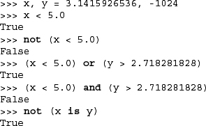
Earlier, we introduced the notion that Python supports multiple comparisons within one expression. These expressions have an implicit and operator joining them together.

We now formally introduce type(). In Python versions earlier than 2.2, type() is a BIF. Since that release, it has become a “factory function.” We will discuss these later on in this chapter, but for now, you may continue to think of type() as a BIF. The syntax for type() is:

In the examples above, we take an integer and a string and obtain their types using the type() BIF; in order to also verify that types themselves are types, we call type() on the output of a type() call.

Note the interesting output from the type() function. It does not look like a typical Python data type, i.e., a number or string, but is something enclosed by greater-than and less-than signs. This syntax is generally a clue that what you are looking at is an object. Objects may implement a printable string representation; however, this is not always the case. In these scenarios where there is no easy way to “display” an object, Python “pretty-prints” a string representation of the object. The format is usually of the form: <object_something_or_another>. Any object displayed in this manner generally gives the object type, an object ID or location, or other pertinent information.

The cmp() BIF CoMPares two objects, say, obj1 and obj2, and returns a negative number (integer) if obj1 is less than obj2, a positive number if obj1 is greater than obj2, and zero if obj1 is equal to obj2. Notice the similarity in return values as C’s strcmp(). The comparison used is the one that applies for that type of object, whether it be a standard type or a user-created class; if the latter, cmp() will call the class’s special __cmp__() method. More on these special methods in Chapter 13, on Python classes. Here are some samples of using the cmp() BIF with numbers and strings.

We will look at using cmp() with other objects later.

The str() STRing and repr() REPResentation BIFs or the single back or reverse quote operator ( `` ) come in very handy if the need arises to either re-create an object through evaluation or obtain a human-readable view of the contents of objects, data values, object types, etc. To use these operations, a Python object is provided as an argument and some type of string representation of that object is returned. In the examples that follow, we take some random Python types and convert them to their string representations.

Although all three are similar in nature and functionality, only repr() and `` do exactly the same thing, and using them will deliver the “official” string representation of an object that can be evaluated as a valid Python expression (using the eval() BIF). In contrast, str() has the job of delivering a “printable” string representation of an object, which may not necessarily be acceptable by eval(), but will look nice in a print statement. There is a caveat that while most return values from repr() can be evaluated, not all can:

The executive summary is that repr() is Python-friendly while str() produces human-friendly output. However, with that said, because both types of string representations coincide so often, on many occasions all three return the exact same string.

Core Note: Why have both repr() and ``?

Occasionally in Python, you will find both an operator and a function that do exactly the same thing. One reason why both an operator and a function exist is that there are times where a function may be more useful than the operator, for example, when you are passing around executable objects like functions and where different functions may be called depending on the data item. Another example is the double-star ( ** ) and pow() BIF, which performs “x to the y power” exponentiation for x ** y or pow(x,y).

Python does not support method or function overloading, so you are responsible for any “introspection” of the objects that your functions are called with. (Also see the Python FAQ 4.75.) Fortunately, we have the type() BIF to help us with just that, introduced earlier in Section 4.3.1.

What’s in a name? Quite a lot, if it is the name of a type. It is often advantageous and/or necessary to base pending computation on the type of object that is received. Fortunately, Python provides a BIF just for that very purpose. type() returns the type for any Python object, not just the standard types. Using the interactive interpreter, let us take a look at some examples of what type() returns when we give it various objects.

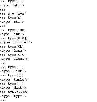
Types and classes were unified in Python 2.2. You will see output different from that above if you are using a version of Python older than 2.2:

In addition to type(), there is another useful BIF called isinstance(). We cover it more formally in Chapter 13 (Object-Oriented Programming), but here we can introduce it to show you how you can use it to help determine the type of an object.

A summary of operators and BIFs common to all basic Python types is given in Table 4.5. The progressing shaded groups indicate hierarchical precedence from highest-to-lowest order. Elements grouped with similar shading all have equal priority. Note that these (and most Python) operators are available as functions via the operator module.

Table 4.5. Standard Type Operators and Built-in Functions

The first way we can categorize the types is by how many objects can be stored in an object of this type. Python’s types, as well as types from most other languages, can hold either single or multiple values. A type which holds a single literal object we will call atomic or scalar storage, and those which can hold multiple objects we will refer to as container storage. (Container objects are also referred to as composite or compound objects in the documentation, but some of these refer to objects other than types, such as class instances.) Container types bring up the additional issue of whether different types of objects can be stored. All of Python’s container types can hold objects of different types. Table 4.6 categorizes Python’s types by storage model.

Table 4.6. Types Categorized by the Storage Model

Although strings may seem like a container type since they “contain” characters (and usually more than one character), they are not considered as such because Python does not have a character type (see Section 4.9). Thus strings are self-contained literals.

Another way of categorizing the standard types is by asking the question, “Once created, can objects be changed, or can their values be updated?” When we introduced Python types early on, we indicated that certain types allow their values to be updated and others do not. Mutable objects are those whose values can be changed, and immutable objects are those whose values cannot be changed. Table 4.7 illustrates which types support updates and which do not.

Table 4.7. Types Categorized by the Update Model

Now after looking at the table, a thought that must immediately come to mind is, “Wait a minute! What do you mean that numbers and strings are immutable? I’ve done things like the following”:

“They sure as heck don’t look immutable to me!” That is true to some degree, but looks can be deceiving. What is really happening behind the scenes is that the original objects are actually being replaced in the above examples. Yes, that is right. Read that again.

Rather than referring to the original objects, new objects with the new values were allocated and (re)assigned to the original variable names, and the old objects were garbage-collected. One can confirm this by using the id() BIF to compare object identities before and after such assignments.

If we added calls to id() in our example above, we may be able to see that the objects are being changed, as below:

Your mileage will vary with regard to the object IDs as they will differ between executions. On the flip side, lists can be modified without replacing the original object, as illustrated in the code below:

Notice how for each change, the ID for the list remained the same.

Although the previous two models of categorizing the types are useful when being introduced to Python, they are not the primary models for differentiating the types. For that purpose, we use the access model. By this, we mean, how do we access the values of our stored data? There are three categories under the access model: direct, sequence, and mapping. The different access models and which types fall into each respective category are given in Table 4.8.

Table 4.8. Types Categorized by the Access Model

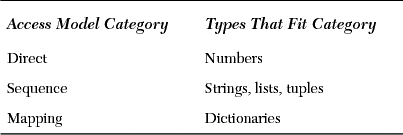
Direct types indicate single-element, non-container types. All numeric types fit into this category.

Sequence types are those whose elements are sequentially accessible via index values starting at 0. Accessed items can be either single elements or in groups, better known as slices. Types that fall into this category include strings, lists, and tuples. As we mentioned before, Python does not support a character type, so, although strings are literals, they are a sequence type because of the ability to access substrings sequentially.

Mapping types are similar to the indexing properties of sequences, except instead of indexing on a sequential numeric offset, elements (values) are unordered and accessed with a key, thus making mapping types a set of hashed key-value pairs.

We will use this primary model in the next chapter by presenting each access model type and what all types in that category have in common (such as operators and BIFs), then discussing each Python standard type that fits into those categories. Any operators, BIFs, and methods unique to a specific type will be highlighted in their respective sections.

So why this side trip to view the same data types from differing perspectives? Well, first of all, why categorize at all? Because of the high-level data structures that Python provides, we need to differentiate the “primitive” types from those that provide more functionality. Another reason is to be clear on what the expected behavior of a type should be. For example, if we minimize the number of times we ask ourselves, “What are the differences between lists and tuples again?” or “What types are immutable and which are not?” then we have done our job. And finally, certain categories have general characteristics that apply to all types in a certain category. A good craftsman (and craftswoman) should know what is available in his or her toolboxes.

The second part of our inquiry asks, “Why all these different models or perspectives”? It seems that there is no one way of classifying all of the data types. They all have crossed relationships with each other, and we feel it best to expose the different sets of relationships shared by all the types. We also want to show how each type is unique in its own right. No two types map the same across all categories. (Of course, all numeric subtypes do, so we are categorizing them together.) Finally, we believe that understanding all these relationships will ultimately play an important implicit role during development. The more you know about each type, the more you are apt to use the correct ones in the parts of your application where they are the most appropriate, and where you can maximize performance.

We summarize by presenting a cross-reference chart (see Table 4.9) that shows all the standard types, the three different models we use for categorization, and where each type fits into these models.

Table 4.9. Categorizing the Standard Types

Python does not have a char type to hold either single character or 8-bit integers. Use strings of length one for characters and integers for 8-bit numbers.

Since Python manages memory for you, there is no need to access pointer addresses. The closest to an address that you can get in Python is by looking at an object’s identity using the id() BIF. Since you have no control over this value, it’s a moot point. However, under Python’s covers, everything is a pointer.

Python’s plain integers are the universal “standard” integer type, obviating the need for three different integer types, e.g., C’s int, short, and long. For the record, Python’s integers are implemented as C longs. Also, since there is a close relationship between Python’s int and long types, users have even fewer things to worry about. You only need to use a single type, the Python integer. Even when the size of an integer is exceed, for example, multiplying two very large numbers, Python automatically gives you a long back instead of overflowing with an error.

C has both a single precision float type and double-precision double type. Python’s float type is actually a C double. Python does not support a single-precision floating point type because its benefits are outweighed by the overhead required to support two types of floating point types. For those wanting more accuracy and willing to give up a wider range of numbers, Python has a decimal floating point number too, but you have to import the decimal module to use the Decimal type. Floats are always estimations. Decimals are exact and arbitrary precision. Decimals make sense concerning things like money where the values are exact. Floats make sense for things that are estimates anyway, such as weights, lengths, and other measurements.