
Chapter Topics
We were introduced to functions in Chapter 2, and we have seen them created and called throughout the text. In this chapter, we will look beyond the basics and give you a full treatment of all the other features associated with functions. In addition to the expected behavior, functions in Python support a variety of invocation styles and argument types, including some functional programming interfaces. We conclude this chapter with a look at Python’s scoping and take an optional side trip into the world of recursion.
Functions are the structured or procedural programming way of organizing the logic in your programs. Large blocks of code can be neatly segregated into manageable chunks, and space is saved by putting oft-repeated code in functions as opposed to multiple copies everywhere—this also helps with consistency because changing the single copy means you do not have to hunt for and make changes to multiple copies of duplicated code. The basics of functions in Python are not much different from those of other languages with which you may be familiar. After a bit of review here in the early part of this chapter, we will focus on what else Python brings to the table.
Functions can appear in different ways ... here is a sampling profile of how you will see functions created, used, or otherwise referenced:
declaration/definition def foo(): print ‘bar’
function object/reference foo
function call/invocation foo()
Functions are often compared to procedures. Both are entities that can be invoked, but the traditional function or “black box,” perhaps taking some or no input parameters, performs some amount of processing, and concludes by sending back a return value to the caller. Some functions are Boolean in nature, returning a “yes” or “no” answer, or, more appropriately, a non-zero or zero value, respectively. Procedures are simply special cases, functions that do not return a value. As you will see below, Python procedures are implied functions because the interpreter implicitly returns a default value of None.
Functions may return a value back to their callers and those that are more procedural in nature do not explicitly return anything at all. Languages that treat procedures as functions usually have a special type or value name for functions that “return nothing.” These functions default to a return type of “void” in C, meaning no value returned. In Python, the equivalent return object type is None.
The hello() function acts as a procedure in the code below, returning no value. If the return value is saved, you will see that its value is None:

Also, like most other languages, you may return only one value/object from a function in Python. One difference is that in returning a container type, it will seem as if you can actually return more than a single object. In other words, you cannot leave the grocery store with multiple items, but you can throw them all in a single shopping bag, which you walk out of the store with, perfectly legal.
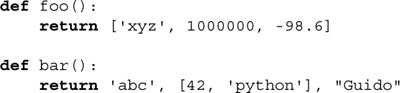
The foo() function returns a list, and the bar() function returns a tuple. Because of the tuple’s syntax of not requiring the enclosing parentheses, it creates the perfect illusion of returning multiple items. If we were to properly enclose the tuple items, the definition of bar() would look like this:
![]()
As far as return values are concerned, tuples can be saved in a number of ways. The following three ways of saving the return values are equivalent:
In the assignments for x, y, z, and a, b, c, each variable will receive its corresponding return value in the order the values are returned. The aTuple assignment takes the entire implied tuple returned from the function. Recall that a tuple can be “unpacked” into individual variables or not at all and its reference assigned directly to a single variable. (Refer back to Section 6.18.3 for a review.)
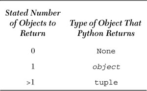
In short, when no items are explicitly returned or if None is returned, then Python returns None. If the function returns exactly one object, then that is the object that Python returns and the type of that object stays the same. If the function returns multiple objects, Python gathers them all together and returns them in a tuple. Yes, we claim that Python is more flexible than languages like C where only one return value is allowed, but in all honesty, Python follows the same tradition. The programmer is just given the impression that he or she can return more than one object. Table 11.1 summarizes the number of items “returned” from a function, and the object that Python actually returns.
Many languages that support functions maintain the notion that a function’s type is the type of its return value. In Python, no direct type correlation can be made since Python is dynamically typed and functions can return values of different types. Because overloading is not a feature, the programmer can use the type() built-in function as a proxy for multiple declarations with different signatures (multiple prototypes of the same overloaded function that differ based on its arguments).
Functions are called using the same pair of parentheses that you are used to. In fact, some consider ( () ) to be a two-character operator, the function operator. As you are probably aware, any input parameters or arguments must be placed between these calling parentheses. Parentheses are also used as part of function declarations to define those arguments. Although we have yet to formally study classes and object-oriented programming, you will discover that the function operator is also used in Python for class instantiation.
The concept of keyword arguments applies only to function invocation. The idea here is for the caller to identify the arguments by parameter name in a function call. This specification allows for arguments to be missing or out-of-order because the interpreter is able to use the provided keywords to match values to parameters.
For a simple example, imagine a function foo(), which has the following pseudocode definition:

For a more realistic example, let us assume you have a function called net_conn() and you know that it takes two parameters, say, host and port:
![]()
Naturally, we can call the function, giving the proper arguments in the correct positional order in which they were declared:
net_conn(’kappa’, 8080)
The host parameter gets the string ’kappa’ and port gets integer 8080. Keyword arguments allow out-of-order parameters, but you must provide the name of the parameter as a “keyword” to have your arguments match up to their corresponding argument names, as in the following:
net_conn(port=8080, host=’chino’)
Keyword arguments may also be used when arguments are allowed to be “missing.” These are related to functions that have default arguments, which we will introduce in the next section.
Default arguments are those that are declared with default values. Parameters that are not passed on a function call are thus allowed and are assigned the default value. We will cover default arguments more formally in Section 11.5.2.
Python also allows the programmer to execute a function without explicitly specifying individual arguments in the call as long as you have grouped the arguments in either a tuple (non-keyword arguments) or a dictionary (keyword arguments), both of which we will explore in this chapter. Basically, you can put all the arguments in either a tuple or a dictionary (or both), and just call a function with those buckets of arguments and not have to explicitly put them in the function call:
func(*tuple_grp_nonkw_args, **dict_grp_kw_args)
The tuple_grp_nonkw_args are the group of non-keyword arguments as a tuple, and the dict_grp_kw_args are a dictionary of keyword arguments. As we already mentioned, we will cover all of these in this chapter, but just be aware of this feature that allows you to stick arguments in tuples and/or dictionaries and be able to call functions without explicitly stating each one by itself in the function call.
In fact, you can give formal arguments, too! These include the standard positional parameters as well as keyword argument, so the full syntax allowed in Python for making a function call is:
![]()
All arguments in this syntax are optional—everything is dependent on the individual function call as far as which parameters to pass to the function. This syntax has effectively deprecated the apply() built-in function. (Prior to Python 1.6, such argument objects could only be passed to apply() with the function object for invocation.)
In our math game in Example 11.1 (easyMath.py), we will use the current function calling convention to generate a two-item argument list to send to the appropriate arithmetic function. (We will also show where apply() would have come in if it had been used.)

The easyMath.py application is basically an arithmetic math quiz game for children where an arithmetic operation—addition or subtraction—is randomly chosen. We use the functional equivalents of these operators, add() and sub(), both found in the operator module. We then generate the list of arguments (two, since these are binary operators/operations). Then random numbers are chosen as the operands. Since we do not want to support negative numbers in this more elementary edition of this application, we sort our list of two numbers in largest-to-smallest order, then call the corresponding function with this argument list and the randomly chosen arithmetic operator to obtain the correct solution to the posed problem.
Our code begins with the usual Unix startup line followed by various imports of the functions that we will be using from the operator and random modules.
The global variables we use in this application are a set of operations and their corresponding functions, and a value indicating how many times (three: 0, 1, 2) we allow the user to enter an incorrect answer before we reveal the solution. The function dictionary uses the operator’s symbol to index into the dictionary, pulling out the appropriate arithmetic function.
The doprob() function is the core engine of the application. It randomly picks an operation and generates the two operands, sorting them from largest-to-smallest order in order to avoid negative numbers for subtraction problems. It then invokes the math function with the values, calculating the correct solution. The user is then prompted with the equation and given three opportunities to enter the correct answer.
Line 10 uses the random.choice() function. Its job is to take a sequence—a string of operation symbols in our case—and randomly choose one item and return it.
Line 11 uses a list comprehension to randomly choose two numbers for our exercise. This example is simple enough such that we could have just called randint() twice to get our operands, i.e., nums = [randint (1,10), randint(1,10)], but we wanted to use a list comprehension so that you could see another example of its use as well as in case we wanted to upgrade this problem to take on more than just two numbers, similar to the reason why instead of cutting and pasting the same piece of code, we put it into a for loop.
Line 12 will only work in Python 2.4 and newer because that is when the reverse flag was added to the list.sort() method (as well as the new sorted() built-in function). If you are using an earlier Python version, you need to either:
• Add an inverse comparison function to get a reverse sort, i.e., lambda x,y: cmp(y, x), or
• Call nums.sort() followed by nums.reverse()
Don’t be afraid of lambda if you have not seen it before. We will cover it in this chapter, but for now, you can think of it as a one-line anonymous function.
Line 13 is where apply() would have been used if you are using Python before 1.6. This call to the appropriate operation function would have been coded as apply(ops[op], nums) instead of ops[op](*nums).
Lines 16-28 represent the controlling loop handling valid and invalid user input. The while loop is “infinite,” running until either the correct answer is given or the number of allowed attempts is exhausted, three in our case. It allows the program to accept erroneous input such as non-numbers, or various keyboard control characters. Once the user exceeds the maximum number of tries, the answer is presented, and the user is “forced” to enter the correct value, not proceeding until that has been done.
The main driver of the application is main(), called from the top level if the script is invoked directly. If imported, the importing function either manages the execution by calling doprob(), or calls main() for program control. main() simply calls doprob() to engage the user in the main functionality of the script and prompts the user to quit or to try another problem.
Since the values and operators are chosen randomly, each execution of easyMath.py should be different. Here is what we got today (oh, and your answers may vary as well!):

Functions are created using the def statement, with a syntax like the following:

The header line consists of the def keyword, the function name, and a set of arguments (if any). The remainder of the def clause consists of an optional but highly recommended documentation string and the required function body suite. We have seen many function declarations throughout this text, and here is another:

Some programming languages differentiate between function declarations and function definitions. A function declaration consists of providing the parser with the function name, and the names (and traditionally the types) of its arguments, without necessarily giving any lines of code for the function, which is usually referred to as the function definition.
In languages where there is a distinction, it is usually because the function definition may belong in a physically different location in the code from the function declaration. Python does not make a distinction between the two, as a function clause is made up of a declarative header line immediately followed by its defining suite.
Like some other high-level languages, Python does not permit you to reference or call a function before it has been declared. We can try a few examples to illustrate this:

If we were to call foo() here, it would fail because bar() has not been declared yet:

We will now define bar(), placing its declaration before foo()’s declaration:
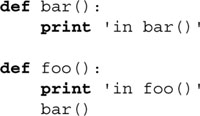
Now we can safely call foo() with no problems:

In fact, we can even declare foo() before bar():
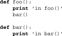
Amazingly enough, this code still works fine with no forward referencing problems:

This piece of code is fine because even though a call to bar() (from foo()) appears before bar()’s definition, foo() itself is not called before bar() is declared. In other words, we declared foo(), then bar(), and then called foo(), but by that time, bar() existed already, so the call succeeds.
Notice that the output of foo() succeeded before the error came about. NameError is the exception that is always raised when any uninitialized identifiers are accessed.
We will briefly discuss namespaces later on in this chapter, especially their relationship to variable scope. There will be a more in-depth treatment of namespaces in the next chapter; however, here we want to point out a basic feature of Python namespaces.
You get a free one with every Python module, class, and function. You can have a variable named x in modules foo and bar, but can use them in your current application upon importing both modules. So even though the same variable name is used in both modules, you are safe because the dotted attribute notation implies a separate namespace for both, i.e., there is no naming conflict in this snippet of code:
import foo, bar
print foo.x + bar.x
Function attributes are another area of Python to use the dotted-attribute notation and have a namespace. (More on namespaces later on in this chapter as well as Chapter 12 on Python modules.)

In foo() above, we create our documentation string as normal, e.g., the first unassigned string after the function declaration. When declaring bar(), we left everything out and just used the dotted-attribute notation to add its doc string as well as another attribute. We can then access the attributes freely. Below is an example with the interactive interpreter. (As you may already be aware, using the built-in function help() gives more of a pretty-printing format than just using the vanilla print of the __doc__ attribute, but you can use either one you wish.)

Notice how we can define the documentation string outside of the function declaration. Yet we can still access it at runtime just like normal. One thing that you cannot do, however, is get access to the attributes in the function declaration. In other words, there is no such thing as a “self” inside a function declaration so that you can make an assignment like __dict__[’version’] = 0.1. The reason for this is because the function object has not even been created yet, but afterward you have the function object and can add to its dictionary in the way we described above ... another free namespace!
Function attributes were added to Python in 2.1, and you can read more about them in PEP 232.
It is perfectly legitimate to create function (object)s inside other functions. That is the definition of an inner or nested function. Because Python now supports statically nested scoping (introduced in 2.1 but standard as of 2.2), inner functions are actually useful now. It made no sense for older versions of Python, which only supported the global and one local scope. So how does one create a nested function?
The (obvious) way to create an inner function is to define a function from within an outer function’s definition (using the def keyword), as in:

If we stick this code in a module, say inner.py, and run it, we get the following output:

One interesting aspect of inner functions is that they are wholly contained inside the outer function’s scope (the places where you can access an object; more on scope later on in this chapter). If there are no outside references to bar(), it cannot be called from anywhere else except inside the outer function, hence the reason for the exception you see at the end of execution in the above code snippet.
Another way of creating a function object while inside a(nother) function is by using the lambda statement. We will cover this later on in section 11.7.1.
Inner functions turn into something special called closures if the definition of an inner function contains a reference to an object defined in an outer function. (It can even be beyond the immediately enclosing outer function too.) We will learn more about closures coming up in Section 11.8.4. In the next section, we will introduce decorators, but the example application also includes a preview of a closure.
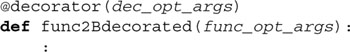
The main motivation behind decorators came from Python object-oriented programming (OOP). Decorators are just “overlays” on top of function calls. These overlays are just additional calls that are applied when a function or method is declared.
The syntax for decorators uses a leading “at-sign” ( @ ) followed by the decorator function name and optional arguments. The line following the decorator declaration is the function being decorated, along with its optional arguments. It looks something like this:
So how (and why) did this syntax come into being? What was the inspiration behind decorators? Well, when static and class methods were added to Python in 2.2, the idiom required to realize them was clumsy, confusing, and makes code less readable, i.e.,

(It was clearly stated for that release that this was not the final syntax anyway.) Within this class declaration, we define a method named staticFoo(). Now since this is intended to become a static method, we leave out the self argument, which is required for standard class methods, as you will see in Chapter 12. The staticmethod() built-in function is then used to “convert” the function into a static method, but note how “sloppy” it looks with def staticFoo() followed by staticFoo = staticmethod (staticFoo). With decorators, you can now replace that piece of code with the following:

Furthermore, decorators can be “stacked” like function calls, so here is a more general example with multiple decorators:
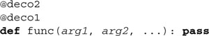
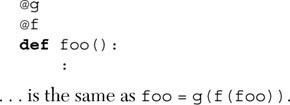
This is equivalent to creating a composite function:
![]()
Function composition in math is defined like this: (g • f)(x) = g(f(x)). For consistency in Python:
Yes the syntax is slightly mind-bending at first, but once you are comfortable with it, the only twist on top of that is when you use decorators with arguments. Without arguments, a decorator like:
@deco
def foo(): pass
... is pretty straightforward:
foo = deco(foo)
Function composition without arguments (as seen above) follows. However, a decorator decomaker() with arguments:
@decomaker(deco_args)
def foo(): pass
... needs to itself return a decorator that takes the function as an argument. In other words, decomaker() does something with deco_args and returns a function object that is a decorator that takes foo as its argument. To put it simply:
foo = decomaker(deco_args)(foo)
Here is an example featuring multiple decorators in which one takes an argument:
@deco1(deco_arg)
@deco2
def func(): pass
This is equivalent to:
func = deco1(deco_arg)(deco2(func))
We hope that if you understand these examples here, things will become much clearer. We present a more useful yet still simple script below where the decorator does not take an argument. Example 11.8 is an intermediate script with a decorator that does take an argument.
We know that decorators are really functions now. We also know that they take function objects. But what will they do with those functions? Generally, when you wrap a function, you eventually call it. The nice thing is that we can do that whenever it is appropriate for our wrapper. We can run some preliminary code before executing the function or some cleanup code afterward, like postmortem analysis. It is up to the programmer. So when you see a decorator function, be prepared to find some code in it, and somewhere embedded within its definition, a call or at least some reference, to the target function.
This feature essentially introduces the concept that Java developers call AOP, or aspect-oriented programming. You can place code in your decorators for concerns that cut across your application. For example, you can use decorators to:
• Introduce logging
• Insert timing logic (aka instrumentation) for monitoring performance
• Add transactional capabilities to functions
The ability to support decorators is very important for creating enterprise applications in Python. You will see that the bullet points above correspond quite closely to our example below as well as Example 11.2.
We have an extremely simple example below, but it should get you started in really understanding how decorators work. This example “decorates” a (useless) function by displaying the time that it was executed. It is a “timestamp decoration” similar to the timestamp server that we discuss in Chapter 16.
Example 11.2. Example of Using a Function Decorator (deco.py)
This demonstration of a decorator (and closures) shows that it is merely a “wrapper” with which to “decorate” (or overlay) a function, returning the altered function object and reassigning it to the original identifier, forever losing access to the original function object.

Running this script, we get the following output:
![]()
Following the startup and module import lines, the tsfunc() function is a decorator that displays a timestamp (to standard output) of when a function is called. It defines an inner function wrappedFunc(), which adds the timestamp and calls the target function. The return value of the decorator is the “wrapped” function.
We define function foo() with an empty body (which does nothing) and decorate it with tsfunc(). We then call it once as a proof-of-concept, wait four seconds, then call it twice more, pausing one second before each invocation.
As a result, after it has been called once, the second time it is called should be five (4 + 1) seconds after the first call, and the third time around should only be one second after that. This corresponds perfectly to the program output seen above.
You can read more about decorators in the Python Language Reference, the “What’s New in Python 2.4” document, and the defining PEP 318. Also, decorators are made available to classes starting in 2.6. See the “What’s New in Python 2.6” document and PEP 3129 for more information.
The concept of function pointers is an advanced topic when learning a language such as C, but not Python where functions are like any other object. They can be referenced (accessed or aliased to other variables), passed as arguments to functions, be elements of container objects such as lists and dictionaries, etc. The one unique characteristic of functions which may set them apart from other objects is that they are callable, i.e., they can be invoked via the function operator. (There are other callables in Python. For more information, see Chapter 14.)
In the description above, we noted that functions can be aliases to other variables. Because all objects are passed by reference, functions are no different. When assigning to another variable, you are assigning the reference to the same object; and if that object is a function, then all aliases to that same object are callable:

When we assigned foo to bar, we are assigning the same function object to bar, thus we can invoke bar() in the same way we call foo(). Be sure you understand the difference between “foo” (reference of the function object) and “foo()” (invocation of the function object).
Taking our reference example a bit further, we can even pass functions in as arguments to other functions for invocation:

Note that it is the function object foo that is being passed to bar(). bar() is the function that actually calls foo() (which has been aliased to the local variable argfunc in the same way that we assigned foo to bar in the previous example). Now let us examine a more realistic example, numconv.py, whose code is given in Example 11.3.
Example 11.3. Passing and Calling (Built-in) Functions (numConv.py)
A more realistic example of passing functions as arguments and invoking them from within the function. This script simply converts a sequence of numbers to the same type using the conversion function that is passed in. In particular, the test() function passes in a built-in function int(), long(), or float() to perform the conversion.
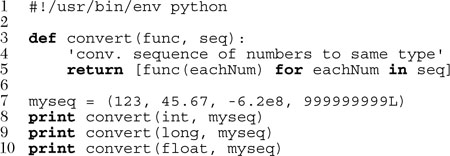
If we were to run this program, we would get the following output:
A Python function’s set of formal arguments consists of all parameters passed to the function on invocation for which there is an exact correspondence to those of the argument list in the function declaration. These arguments include all required arguments (passed to the function in correct positional order), keyword arguments (passed in or out of order, but which have keywords present to match their values to their proper positions in the argument list), and all arguments that have default values that may or may not be part of the function call. For all of these cases, a name is created for that value in the (newly created) local namespace and it can be accessed as soon as the function begins execution.
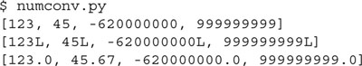
These are the standard vanilla parameters that we are all familiar with. Positional arguments must be passed in the exact order in which they are defined for the functions that are called. Also, without the presence of any default arguments (see next section), the exact number of arguments passed to a function (call) must be exactly the number declared:
The foo() function has one positional argument. That means that any call to foo() must have exactly one argument, no more, no less. You will become extremely familiar with TypeError otherwise. Note how informative the Python errors are. As a general rule, all positional arguments for a function must be provided whenever you call it. They may be passed into the function call in position or out of position, granted that a keyword argument is provided to match it to its proper position in the argument list (review Section 11.2.2). Default arguments, however, do not have to be provided because of their nature.
Default arguments are parameters that are defined to have a default value if one is not provided in the function call for that argument. Such definitions are given in the function declaration header line. C++ supports default arguments too and has the same syntax as Python: the argument name is followed by an “assignment” of its default value. This assignment is merely a syntactical way of indicating that this assignment will occur if no value is passed in for that argument.
The syntax for declaring variables with default values in Python is such that all positional arguments must come before any default arguments:

Each default argument is followed by an assignment statement of its default value. If no value is given during a function call, then this assignment is realized.
Default arguments add a wonderful level of robustness to applications because they allow for some flexibility that is not offered by the standard positional parameters. That gift comes in the form of simplicity for the applications programmer. Life is not as complicated when there are a fewer number of parameters that one needs to worry about. This is especially helpful when one is new to an API interface and does not have enough knowledge to provide more targeted values as arguments.
The concept of using default arguments is analogous to the process of installing software on your computer. How often does one choose the “default install” over the “custom install?” I would say probably almost always. It is a matter of convenience and know-how, not to mention a time-saver. And if you are one of those gurus who always chooses the custom install, please keep in mind that you are one of the minority.
Another advantage goes to the developers, who are given more control over the software they create for their consumers. When providing default values, they can selectively choose the “best” default value possible, thereby hoping to give the user some freedom of not having to make that choice. Over time, as the users becomes more familiar with the system or API, they may eventually be able to provide their own parameter values, no longer requiring the use of “training wheels.”
Here is one example where a default argument comes in handy and has some usefulness in the growing electronic commerce industry:

In the example above, the taxMe() function takes the cost of an item and produces a total sale amount with sales tax added. The cost is a required parameter while the tax rate is a default argument (in our example, 8.25%). Perhaps you are an online retail merchant, with most of your customers coming from the same state or county as your business. Consumers from locations with different tax rates would like to see their purchase totals with their corresponding sales tax rates. To override the default, all you have to do is provide your argument value, such as the case with taxMe(100, 0.05) in the above example. By specifying a rate of 5%, you provided an argument as the rate parameter, thereby overriding or bypassing its default value of 0.0825.
All required parameters must be placed before any default arguments. Why? Simply because they are mandatory, whereas default arguments are not. Syntactically, it would be impossible for the interpreter to decide which values match which arguments if mixed modes were allowed. A SyntaxError is raised if the arguments are not given in the correct order:

Let us take a look at keyword arguments again, using our old friend net_conn().
![]()
As you will recall, this is where you can provide your arguments out of order (positionally) if you name the arguments. With the above declarations, we can make the following (regular) positional or keyword argument calls:
• net_conn('kappa', 8000)
• net_conn(port=8080, host='chino')
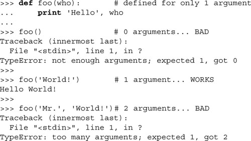
However, if we bring default arguments into the equation, things change, although the above calls are still valid. Let us modify the declaration of net_conn() such that the port parameter has a default value of 80 and add another argument named stype (for server type) with a default value of ’tcp’:
![]()
We have just expanded the number of ways we can call net_conn(). The following are all valid calls to net_conn():
What is the one constant we see in all of the above examples? The sole required parameter, host. There is no default value for host, thus it is expected in all calls to net_conn().
Keyword arguments prove useful for providing for out-of-order positional arguments, but, coupled with default arguments, they can also be used to “skip over” missing arguments as well, as evidenced from our examples above.
We will now present yet another example of where a default argument may prove beneficial. The grabWeb.py script, given in Example 11.4, is a simple script whose main purpose is to grab a Web page from the Internet and temporarily store it to a local file for analysis. This type of application can be used to test the integrity of a Web site’s pages or to monitor the load on a server (by measuring connectability or download speed). The process() function can be anything we want, presenting an infinite number of uses. The one we chose for this exercise displays the first and last non-blank lines of the retrieved Web page. Although this particular example may not prove too useful in the real world, you can imagine what kinds of applications you can build on top of this code.
Example 11.4. Grabbing Web Pages (grabWeb.py)
This script downloads a Web page (defaults to local www server) and displays the first and last non-blank lines of the HTML file. Flexibility is added due to both default arguments of the download() function, which will allow overriding with different URLs or specification of a different processing function.
Running this script in our environment gives the following output, although your mileage will definitely vary since you will be viewing a completely different Web page altogether.

There may be situations where your function is required to process an unknown number of arguments. These are called variable-length argument lists. Variable-length arguments are not named explicitly in function declarations because the number of arguments is unknown before runtime (and even during execution, the number of arguments may be different on successive calls), an obvious difference from formal arguments (positional and default), which are named in function declarations. Python supports variable-length arguments in two ways because function calls provide for both keyword and non-keyword argument types.
In Section 11.2.4, we looked at how you can use the * and ** characters in function calls to specify grouped sets of arguments, non-keyword and keyword arguments. In this section, we will see the same symbols again, but this time in function declarations, to signify the receipt of such arguments when functions are called. This syntax allows functions to accept more than just the declared formal arguments as defined in the function declaration.
When a function is invoked, all formal (required and default) arguments are assigned to their corresponding local variables as given in the function declaration. The remaining non-keyword variable arguments are inserted in order into a tuple for access. Perhaps you are familiar with “varargs” in C (i.e., va_list, va_arg, and the ellipsis [ ... ]). Python provides equivalent support—iterating over the tuple elements is the same as using va_arg in C. For those who are not familiar with C or varargs, they just represent the syntax for accepting a variable (not fixed) number of arguments passed in a function call.
The variable-length argument tuple must follow all positional and default parameters, and the general syntax for functions with tuple or non-keyword variable arguments is as follows:

The asterisk operator ( * ) is placed in front of the variable that will hold all remaining arguments once all the formal parameters if have been exhausted. The tuple is empty if there are no additional arguments given.
As we saw earlier, a TypeError exception is generated whenever an incorrect number of arguments is given in the function invocation. By adding a variable argument list variable at the end, we can handle the situation when more than enough arguments are passed to the function because all the extra (non-keyword) ones will be added to the variable argument tuple. (Extra keyword arguments require a keyword variable argument parameter [see the next section].)
As expected, all formal arguments must precede informal arguments for the same reason that positional arguments must come before keyword arguments.

We will now invoke this function to show how variable argument tuples work:

In the case where we have a variable number or extra set of keyword arguments, these are placed into a dictionary where the “keyworded” argument variable names are the keys, and the arguments are their corresponding values. Why must it be a dictionary? Because a pair of items is given for every argument—the name of the argument and its value—it is a natural fit to use a dictionary to hold these arguments. Here is the syntax of function definitions that use the variable argument dictionary for extra keyword arguments:

To differentiate keyword variable arguments from non-keyword informal arguments, a double asterisk ( ** ) is used. The ** is overloaded so as not to be confused with exponentiation. The keyword variable argument dictionary should be the last parameter of the function definition prepended with the ’**’. We now present an example of how to use such a dictionary:

Executing this code in the interpreter, we get the following output:

Both keyword and non-keyword variable arguments may be used in the same function as long as the keyword dictionary is last and is preceded by the non-keyword tuple, as in the following example:

Calling our function within the interpreter, we get the following output:

Above in Section 11.2.4, we introduced the use of * and ** to specify sets of arguments in a function call. Here we will show you more examples of that syntax, with a slight bias toward functions accepting variable arguments.
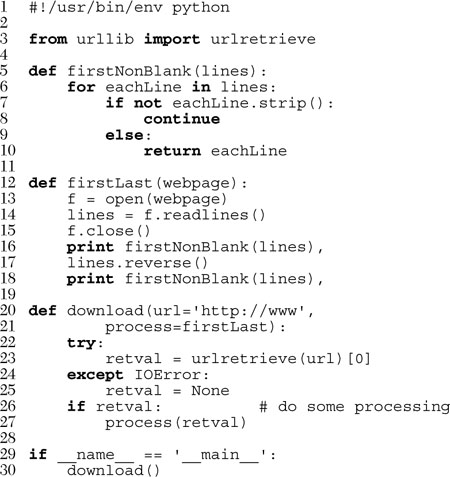
We will now use our friend newfoo(), defined in the previous section, to test the new calling syntax. Our first call to newfoo() will use the old-style method of listing all arguments individually, even the variable arguments that follow all the formal arguments:
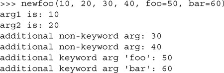
We will now make a similar call; however, instead of listing the variable arguments individually, we will put the non-keyword arguments in a tuple and the keyword arguments in a dictionary to make the call:

Finally, we will make another call but build our tuple and dictionary outside of the function invocation:
Notice how our tuple and dictionary arguments make only a subset of the final tuple and dictionary received within the function call. The additional non-keyword value ’3’ and keyword pairs for ’x’ and ’y’ were also included in the final argument lists even though they were not part of the ’*’ and ’**’ variable argument parameters.
Prior to 1.6, variable objects could only be passed to apply() with the function object for invocation. This current calling syntax effectively obsoletes the use of apply(). Below is an example of using these symbols to call any function object with any type of parameter set.
Another useful application of functional programming comes in terms of debugging or performance measurement. You are working on functions that need to be fully tested or run through regressions every night, or that need to be timed over many iterations for potential improvements. All you need to do is to create a diagnostic function that sets up the test environment, then calls the function in question. Because this system should be flexible, you want to allow the testee function to be passed in as an argument. So a pair of such functions, timeit() and testit(), would probably be useful to the software developer today.
We will now present the source code to one such example of a testit() function (see Example 11.5). We will leave a timeit() function as an exercise for the reader (see Exercise 11.12).
This module provides an execution test environment for functions. The testit() function takes a function and arguments, then invokes that function with the given arguments under the watch of an exception handler. If the function completes successfully, a True return value packaged with the return value of the function is sent back to the caller. Any failure causes False to be returned along with the reason for the exception. (Exception is the root class for all runtime exceptions; review Chapter 10 for details.)
Example 11.5. Testing Functions (testit.py)
testit() invokes a given function with its arguments, returning True packaged with the return value of the function on success or False with the cause of failure.

The unit tester function test() runs a set of numeric conversion functions on an input set of four numbers. There are two failure cases in this test set to confirm such functionality. Here is the output of running the script:

Python is not and will probably not ever claim to be a functional programming language, but it does support a number of valuable functional programming constructs. There are also some that behave like functional programming mechanisms but may not be traditionally considered as such. What Python does provide comes in the form of four built-in functions and lambda expressions.
Python allows one to create anonymous functions using the lambda keyword. They are “anonymous” because they are not declared in the standard manner, i.e., using the def statement. (Unless assigned to a local variable, such objects do not create a name in any namespace either.) However, as functions, they may also have arguments. An entire lambda “statement” represents an expression, and the body of that expression must also be given on the same line as the declaration. We now present the syntax for anonymous functions:
lambda [arg1[, arg2, ... argN]]: expression
Arguments are optional, and if used, are usually part of the expression as well.
Core Note: lambda expression returns callable function object

Calling lambda with an appropriate expression yields a function object that can be used like any other function. They can be passed to other functions, aliased with additional references, be members of container objects, and as callable objects, be invoked (with any arguments, if necessary). When called, these objects will yield a result equivalent to the same expression if given the same arguments. They are indistinguishable from functions that return the evaluation of an equivalent expression.
Before we look at any examples using lambda, we would like to review single-line statements and then show the resemblances to lambda expressions.
![]()
The above function takes no arguments and always returns True. Single line functions in Python may be written on the same line as the header. Given that, we can rewrite our true() function so that it looks something like the following:
def true(): return True
We will present the named functions in this manner for the duration of this chapter because it helps one visualize their lambda equivalents. For our true() function, the equivalent expression (no arguments, returns True) using lambda is:
lambda :True
Usage of the named true() function is fairly obvious, but not for lambda. Do we just use it as is, or do we need to assign it somewhere? A lambda function by itself serves no purpose, as we see here:
>>> lambda :True
<function <lambda> at f09ba0>
In the above example, we simply used lambda to create a function (object), but did not save it anywhere nor did we call it. The reference count for this function object is set to True on creation of the function object, but because no reference is saved, goes back down to zero and is garbage-collected. To keep the object around, we can save it into a variable and invoke it any time after. Perhaps now is a good opportunity:
>>> true = lambda :True
>>> true()
True
Assigning it looks much more useful here. Likewise, we can assign lambda expressions to a data structure such as a list or tuple where, based on some input criteria, we can choose which function to execute as well as what the arguments would be. (In the next section, we will show how to use lambda expressions with functional programming constructs.)
Let us now design a function that takes two numeric or string arguments and returns the sum for numbers or the concatenated string. We will show the standard function first, followed by its unnamed equivalent.
def add(x, y): return x + y ⇔ lambda x, y: x + y
Default and variable arguments are permitted as well, as indicated in the following examples:
![]()
Seeing is one thing, so we will now try to make you believe by showing how you can try them in the interpreter:

One final word on lambda: Although it appears that lambda is a one-line version of a function, it is not equivalent to an “inline” statement in C++, whose purpose is bypassing function stack allocation during invocation for performance reasons. A lambda expression works just like a function, creating a frame object when called.
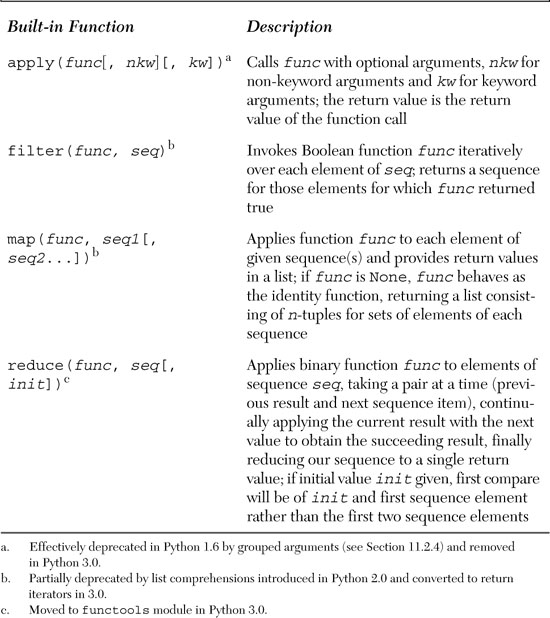
In this section, we will look at the apply(), filter(), map(), and reduce() built-in functions as well as give some examples to show how they can be used. These functions provide the functional programming features found in Python. A summary of these functions is given in Table 11.2. All take a function object to somehow invoke.
As you may imagine, lambda functions fit nicely into applications using any of these functions because all of them take a function object with which to execute, and lambda provides a mechanism for creating functions on the fly.
As mentioned before, the calling syntax for functions, which now allow for a tuple of variable arguments as well as a dictionary of keyword variable arguments, effectively deprecates apply( ) as of Python 1.6. The function will be phased out and eventually removed in a future version of Python. We mention it here for historical purposes as well as for those maintaining code that uses apply( ).
The second built-in function we examine in this chapter is filter( ). Imagine going to an orchard and leaving with a bag of apples you picked off the trees. Wouldn’t it be nice if you could run the entire bag through a filter to keep just the good ones? That is the main premise of the filter( ) function.
Given a sequence of objects and a “filtering” function, run each item of the sequence through the filter, and keep only the ones that the function returns true for. The filter() function calls the given Boolean function for each item of the provided sequence. Each item for which filter() returns a non-zero (true) value is appended to a list. The object that is returned is a “filtered” sequence of the original.
If we were to code filter( ) in pure Python, it might look something like this:

One way to understand filter() better is by visualizing its behavior. Figure 11-1 attempts to do just that.

In Figure 11-1, we observe our original sequence at the top, items seq[0], seq[1], ... seq[N-1] for a sequence of size N. For each call to bool_func(), i.e., bool_func (seq [0]), bool_func (seq [1]), etc., a return value of False or True comes back (as per the definition of a Boolean function—ensure that indeed your function does return one or the other). If bool_func() returns True for any sequence item, that element is inserted into the return sequence. When iteration over the entire sequence has been completed, filter() returns the newly created sequence.
We present below a script that shows one way to use filter() to obtain a short list of random odd numbers. The script generates a larger set of random numbers first, then filters out all the even numbers, leaving us with the desired dataset. When we first coded this example, oddnogen.py looked like the following:
This code snippet contains a function odd() which returns True if the numeric argument that was passed to it was odd and False otherwise. The main portion of the snippet creates a list of nine random numbers in the range 1–99. [Note that random.randint() is inclusive and that we could have used the equivalent random.randrange(1, 100) which is recommended because it has the same calling convention as the built-in function range().] Then filter() does its work: call odd() on each element of the list allNums and return a new list containing just those items of allNums for which odd() returned True, and that new list is then displayed to the user with print.
Importing and running this module several times, we get the following output:

We notice on second glance that odd() is simple enough to be replaced by a lambda expression:

We have already mentioned how list comprehensions can be a suitable replacement for filter() so here it is:
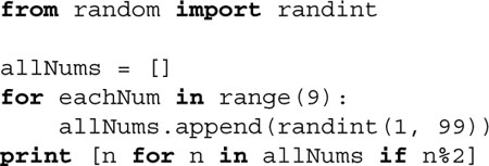
We can further simplify our code by integrating another list comprehension to put together our final list. As you can see below, because of the flexible syntax of list comps, there is no longer a need for intermediate variables. (To make things fit, we import randint() with a shorter name into our code.)
![]()
Although longer than it should be, the line of code making up the core part of this example is not as obfuscated as one might think.
The map() built-in function is similar to filter() in that it can process a sequence through a function. However, unlike filter(), map() “maps” the function call to each sequence item and returns a list consisting of all the return values.
In its simplest form, map() takes a function and sequence, applies the function to each item of the sequence, and creates a return value list that is comprised of each application of the function. So if your mapping function is to add 2 to each number that comes in and you feed that function to map() along with a list of numbers, the resulting list returned is the same set of numbers as the original, but with 2 added to each number. If we were to code how this simple form of map() works in Python, it might look something like the code below that is illustrated in Figure 11-2.


We can whip up a few quick lambda functions to show you how map() works on real data:

We have also discussed how map () can sometimes can be replaced by list comprehensions, so here we refactor our two examples above.
The more general form of map() can take more than a single sequence as its input. If this is the case, then map() will iterate through each sequence in parallel. On the first invocation, it will bundle the first element of each sequence into a tuple, apply the func function to it, and return the result as a tuple into the mapped_seq mapped sequence that is finally returned as a whole when map() has completed execution.
Figure 11-2 illustrated how map() works with a single sequence. If we used map() with M sequences of N objects each, our previous diagram would be converted to something like the diagram presented in Figure 11-3.

Here are several examples using map() with multiple sequences:
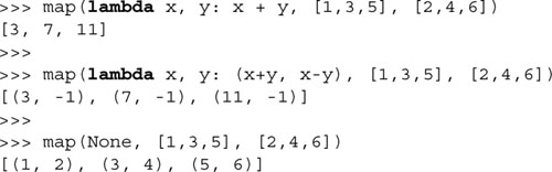
The last example above uses map() and a function object of None to merge elements of unrelated sequences together. This idiom was so commonly used prior to Python 2.0 that a new built-in function, zip(), was added just to address it:
>>> zip([1,3,5], [2,4,6])
[(1, 2), (3, 4), (5, 6)]
The final functional programming piece is reduce(), which takes a binary function (a function that takes two values, performs some calculation and returns one value as output), a sequence, and an optional initializer, and methodologically “reduces” the contents of that list down to a single value, hence its name. In other languages, this concept is known as folding.
It does this by taking the first two elements of the sequence and passing them to the binary function to obtain a single value. It then takes this value and the next item of the sequence to get yet another value, and so on until the sequence is exhausted and one final value is computed.
You may try to visualize reduce() as the following equivalence example:
![]()
Some argue that the “proper functional” use of reduce() requires only one item to be taken at a time for reduce(). In our first iteration above, we took two items because we did not have a “result” from the previous values (because we did not have any previous values). This is where the optional initializer comes in (see the init variable below). If the initializer is given, then the first iteration is performed on the initializer and the first item of the sequence, and follows normally from there.
If we were to try to implement reduce() in pure Python, it might look something like this:

This may be the most difficult of the four conceptually, so we should again show you an example as well as a functional diagram (see Figure 11-4). The “hello world” of reduce() is its use of a simple addition function or its lambda equivalent seen earlier in this chapter:

• def mySum(x,y): return x+y
• lambda x,y: x+y
Given a list, we can get the sum of all the values by simply creating a loop, iteratively going through the list, adding the current element to a running subtotal, and being presented with the result once the loop has completed:

Using lambda and reduce(), we can do the same thing on a single line:
![]()
The reduce() function performs the following mathematical operations given the input above:
((((0 + 1) + 2) + 3) + 4) ⇒ 10
It takes the first two elements of the list (0 and 1), calls mySum() to get 1, then calls mySum() again with that result and the next item 2, gets the result from that, pairs it with the next item 3 and calls mySum(), and finally takes the entire subtotal and calls mySum() with 4 to obtain 10, which is the final return value.
The notion of currying combines the concepts of functional programming and default and variable arguments together. A function taking N arguments that is “curried” embalms the first argument as a fixed parameter and returns another function object taking (the remaining) N-1 arguments, akin to the actions of the LISP primitive functions car and cdr, respectively. Currying can be generalized into partial function application (PFA), in which any number (and order) of arguments is parlayed into another function object with the remainder of the arguments to be supplied later.
In a way, this seems similar to default arguments where if arguments are not provided, they take on a “default” value. In the case of PFAs, the arguments do not have a default value for all calls to a function, only to a specific set of calls. You can have multiple partial function calls, each of which may pass in different arguments to the function, hence the reason why default arguments cannot be used.
This feature was introduced in Python 2.5 and made available to users via the functools module.
How about creating a simple little example? Let us take two simple functions add() and mul(), both found in the operator module. These are just functional interfaces to the + and * operators that we are already familiar with, e.g., add(x, y) is the same as x + y. Say that we wanted to add one to a number or multiply another by 100 quite often in our applications.
Rather than having multiple calls like add(1, foo), add(1, bar), mul(100, foo), mul(100, bar), would it not be nice to just have existing functions that simplify the function call, i.e., add1(foo), add1(bar), mul100(foo), mul100(bar), but without having to write functions add1() and mul100()? Well, now you can with PFAs. You can create a PFA by using the partial() function found in the functional module:

This example may or may not open your eyes to the power of PFAs, but we have to start somewhere. PFAs are best used when calling functions that take many parameters. It is also easier to use PFAs with keyword arguments, because specific arguments can be given explicitly, either as curried arguments, or those more “variable” that are passed in at runtime, and we do not have to worry about ordering. Below is an example from the Python documentation for use in applications where binary data (as strings) need to be converted to integers fairly often:

This example uses the int() built-in function and fixes the base to 2 specifically for binary string conversion. Now instead of multiple calls to int() all with the same second parameter (of 2), e.g., int(’10010’, 2), we can simply use our new baseTwo() function with a single argument. Good style is also followed because it adds a documentation string to the “new (partial) function,” and it is also another good use of “function attributes” (see Section 11.3.4 above). One important thing to note is that the keyword argument base is required here.
If you create the partial function without the base keyword, e.g., baseTwoBAD = partial(int, 2), it would pass the arguments to int() in the wrong order because the fixed arguments are always placed to the left of the runtime arguments, meaning that baseTwoBAD(x) == int(2, x). If you call it, it would pass in 2 as the number to convert and the base as ’10010’, resulting in an exception:
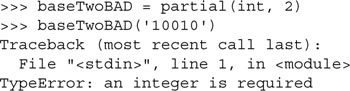
With the keyword in place, the order is preserved properly since, as you know, keyword arguments always come after the formal arguments, so baseTwo(x) == int(x, base=2).
PFAs also extended to all callables like classes and methods. An excellent example of using PFAs is in providing “partial-GUI templating.” GUI widgets often have many parameters, such as text, length, maximum size, background and foreground colors, both active and otherwise, etc. If we wanted to “fix” some of those arguments, such as making all text labels be in white letters on a blue background, you can customize it exactly that way into a pseudo template for similar objects.
Example 11.6. Partial Function Application GUI (pfaGUI.py)
This a more useful example of partial function application, or more accurately, “partial class instantiation” in this case . . . why?

In lines 7-8, we create the “partial class instantiator” (because that is what it is instead of a partial function) for Tkinter.Button, fixing the parent window argument root and both foreground and background colors. We create two buttons b1 and b2 matching this template providing only the text label as unique to each. The quit button (lines 11-12) is slightly more customized, taking on a different background color (red, which overrides the blue default) and installing a callback to close the window when it is pressed. (The other two buttons have no function when they are pressed.)
Without the MyButton “template,” you would have to use the “full” syntax each time (because you are still not giving all the arguments as there are plenty of parameters you are not passing that have default values):

Here is a snapshot of what this simple GUI looks like:

Why bother with so much repetition when your code can be more compact and easy to read? You can find out more about GUI programming in Chapter 18 (Section 18.3.5), where we feature a longer example of using PFAs.
From what you have seen so far, you can see that PFA takes on the flavors of templating and “style-sheeting” in terms of providing defaults in a more functional programming environment. You can read more about them in the documentation for the functools module documentation found in the Python Library Reference, the “What’s New in Python 2.5” document, and the specifying PEP 309.
The scope of an identifier is defined to be the portion of the program where its declaration applies, or what we refer to as “variable visibility.” In other words, it is like asking yourself in which parts of a program do you have access to a specific identifier. Variables either have local or global scope.
Variables defined within a function have local scope, and those at the highest level in a module have global scope. In their famous “dragon” book on compiler theory, Aho, Sethi, and Ullman summarize it this way:
“The portion of the program to which a declaration applies is called the scope of that declaration. An occurrence of a name in a procedure is said to be local to the procedure if it is in the scope of a declaration within the procedure; otherwise, the occurrence is said to be nonlocal.”
One characteristic of global variables is that unless deleted, they have a lifespan that lasts as long as the script that is running and whose values are accessible to all functions, whereas local variables, like the stack frame they reside in, live temporarily, only as long as the functions they are defined in are currently active. When a function call is made, its local variables come into scope as they are declared. At that time, a new local name is created for that object, and once that function has completed and the frame deallocated, that variable will go out of scope.

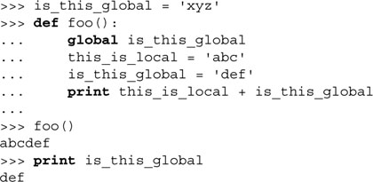
In the above example, global_str is a global variable while local_str is a local variable. The foo() function has access to both global and local variables while the main block of code has access only to global variables.
Core Note: Searching for identifiers (aka variables, names, etc.)
When searching for an identifier, Python searches the local scope first. If the name is not found within the local scope, then an identifier must be found in the global scope or else a NameError exception is raised.
A variable’s scope is related to the namespace in which it resides. We will cover namespaces formally in Chapter 12; suffice it to say for now that namespaces are just naming domains that map names to objects, a virtual set of what variable names are currently in use, if you will. The concept of scope relates to the namespace search order that is used to find a variable. All names in the local namespace are within the local scope when a function is executing. That is the first namespace searched when looking for a variable. If it is not found there, then perhaps a globally scoped variable with that name can be found. These variables are stored (and searched) in the global and built-in namespaces.
It is possible to “hide” or override a global variable just by creating a local one. Recall that the local namespace is searched first, being in its local scope. If the name is found, the search does not continue to search for a globally scoped variable, hence overriding any matching name in either the global or built-in namespaces.
Also, be careful when using local variables with the same names as global variables. If you use such names in a function (to access the global value) before you assign the local value, you will get an exception (NameError or UnboundLocalError), depending on which version of Python you are using.
Global variable names can be overridden by local variables if they are declared within the function. Here is another example, similar to the first, but the global and local nature of the variable are not as clear.

It gave the following output:
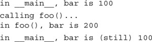
Our local bar pushed the global bar out of the local scope. To specifically reference a named global variable, one must use the global statement. The syntax for global is:
global var1[, var2[, ... varN]]]
Modifying the example above, we can update our code so that we use the global version of is_this_global rather than create a new local variable.
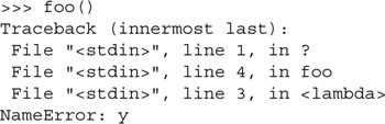
Python syntactically supports multiple levels of functional nesting, and as of Python 2.1, matching statically nested scoping. However, in versions prior to 2.1, a maximum of two scopes was imposed: a function’s local scope and the global scope. Even though more levels of functional nesting exist, you could not access more than two scopes:
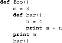
Although this code executes perfectly fine today ...
>>> foo()
3
7
... executing it resulted in errors in Python before 2.1:

The access to foo()’s local variable m within function bar() is illegal because m is declared local to foo(). The only scopes accessible from bar() are bar()’s local scope and the global scope. foo()’s local scope is not included in that short list of two. Note that the output for the “print m” statement succeeded, and it is the function call to bar() that fails. Fortunately with Python’s current nested scoping rules, this is not a problem today.
With Python’s statically nested scoping, it becomes useful to define inner functions as we have seen earlier. In the next section, we will focus on scope and lambda, but inner functions also suffered the same problem before Python 2.1 when the scoping rules changed to what they are today.
If references are made from inside an inner function to an object defined in any outer scope (but not in the global scope), the inner function then is known as a closure. The variables defined in the outer function but used or referred to by the inner function are called free variables. Closures are an important concept in functional programming languages, with Scheme and Haskell being two of them. Closures are syntactically simple (as simple as inner functions) yet still very powerful.
A closure combines an inner function’s own code and scope along with the scope of an outer function. Closure lexical variables do not belong to the global namespace scope or the local one—they belong to someone else’s namespace and carry an “on the road” kind of scope. (Note that they differ from objects in that those variables live in an object’s namespace while closure variables live in a function’s namespace and scope.) So why would you want to use closures?
Closures are useful for setting up calculations, hiding state, letting you move around function objects and scope at will. Closures come in handy in GUI or event-driven programming where a lot of APIs support callbacks. The same applies for retrieving database rows and processing the data in the exact same manner. Callbacks are just functions. Closures are functions, too, but they carry some additional scope with them. They are just functions with an extra feature ... another scope.
You will probably feel that the use of closures draws a strong parallel to partial function application as introduced earlier in this chapter, but PFA is really more like currying than the use of closures because it is not as much as about function calling as it is about using variables defined in another scope.
Below is a short example of using closures. We will simulate a counter and also simulate making an integer mutable by enclosing it as a single element of a list.
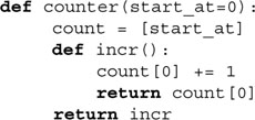
The only thing counter() does is to accept an initial value to start counting at and assigns it as the sole member of the list count. Then an incr() inner function is defined. By using the variable count inside it, we have created a closure because it now carries with it the scope of counter(). incr() increments the running count and returns it. Then the final magic is that counter() returns incr, a (callable) function object.
If we run this interactively, we get the output below—note how similar it looks to instantiating a counter object and executing the instance:

The one difference is that we were able to do something that previously required us to write a class, and not only that, but to have to override the __call__() special method of that class to make its instances callable. Here we were able to do it with a pair of functions.
Now, in many cases, a class is the right thing to use. Closures are more appropriate in cases whenever you need a callback that has to have its own scope, especially if it is something small and simple, and often, clever. As usual, if you use a closure, it is a good idea to comment your code and/or use doc strings to explain what you are doing.
The next two sections contain material for advanced readers ... feel free to skip it if you wish. We will discuss how you can track down free variables with a function’s func_closure attribute. Here is a code snippet that demonstrates it.
If we run this piece of code, we get the following output:


This script starts by creating a template to output a variable: its name, ID, and value, and then sets global variables w, x, y, and z. We define the template so that we do not have to copy the same output format string multiple times.
The definition of the f1() function includes creating local variables x, y, and z plus the definition of an inner function f2(). (Note that all local variables shadow or hide accessing their equivalently named global variables.) If f2() uses any variables that are defined in f1()’s scope, i.e., not global and not local to f2(), those represent free variables, and they will be tracked by f1.func_closure.
Practically duplicating the code for f1(), these lines do the same for f2(), which defines locals y and z plus an inner function f3(). Again, note that the locals here shadow globals as well as those in intermediate localized scopes, e.g., f1()’s. If there are any free variables for f3(), they will be displayed here.
You will no doubt notice that references to free variables are stored in cell objects, or simply, cells. What are these guys? Cells are basically a way to keep references to free variables alive after their defining scope(s) have completed (and are no longer on the stack).
For example, let us assume that function f3() has been passed to some other function so that it can be called later, even after f2() has completed. You do not want to have f2()’s stack frame around because that will keep all of f2()’s variables alive even if we are only interested in the free variables used by f3(). Cells hold on to the free variables so that the rest of f2() can be deallocated.
This block represents the definition of f3(), which creates a local variable z. We then display w, x, y, z, all chased down from the innermost scope outward. The variable w cannot be found in f3(), f2(), or f1(), therefore, it is a global. The variable x is not found in f3() or f2(), so it is a closure variable from f1(). Similarly, y is a closure variable from f2(), and finally, z is local to f3().
The rest of main() attempts to display closure variables for f1(), but it will never happen since there are no scopes in between the global scope and f1()’s—there is no scope that f1() can borrow from, ergo no closure can be created—so the conditional expression on line 34 will never evaluate to True. This code is just here for decorative purposes.
We saw a simple example of using closures and decorators in back in Section 11.3.6, deco.py. The following is a slightly more advanced example, to show you the real power of closures. The application “logs” function calls. The user chooses whether they want to log a function call before or after it has been invoked. If post-log is chosen, the execution time is also displayed.
Example 11.8. Logging Function Calls with Closures (funcLog.py)
This example shows a decorator that takes an argument that ultimately determines which closure will be used. Also featured is the power of closures.
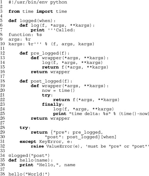
If you execute this script, you will get output similar to the following:
This body of code represents the core part of the logged() function, whose responsibility it is to take the user’s request as to when the function call should be logged. Should it be before the target function is called or after? logged() has three helper inner functions defined within its definition: log(), pre_logged(), and post_logged().
log() is the function that does the actual logging. It just displays to standard output the name of the function and its arguments. If you were to use this function “in the real world,” you would most likely send this output to a file, a database, or perhaps standard error (sys.stderr).
The last part of logged() in lines 28-32 is actually the first lines of code in the function that are not function declarations. It reads the user’s selection when, and returns one of the *logged() functions so that it can then be called with the target function to wrap it.
pre_logged() and post_logged() will both wrap the target function and log it in accordance with its name, e.g., post_logged() will log the function call after the target function has executed while pre_logged() does it before execution.
Depending on the user’s selection, one of pre_logged() and post_logged() will be returned. When the decorator is called, it evaluates the decorator function first along with its argument. e.g., logged(when). Then the returned function object is called with the target function as its parameter, e.g., pre_logged(f) or post_logged(f).
Both *logged() functions include a closure named wrapper(). It calls the target function while logging it as appropriate. The functions return the wrapped function object, which then is reassigned to the original target function identifier.
The main part of this script simply decorates the hello() function and executes it with the modified function object. When you call hello() on line 38, it is not the same as the function object that was created on line 35. The decorator on line 34 wraps the original function object with the specified decoration and returns a wrapped version of hello().
Python’s lambda anonymous functions follow the same scoping rules as standard functions. A lambda expression defines a new scope, just like a function definition, so the scope is inaccessible to any other part of the program except for that local lambda/function.
Those lambda expressions declared local to a function are accessible only within that function; however, the expression in the lambda statement has the same scope access as the function. You can also think of a function and a lambda expression as siblings.

We know that this code works fine now ...
>>> foo()
15
... however, we must again look to the past to see an extremely common idiom that was necessary to get code to work in older versions of Python. Before 2.1, we would get an error like what you see below because while the function and lambda have access to global variables, neither has access to the other’s local scopes:
In the example above, although the lambda expression was created in the local scope of foo(), it has access to only two scopes: its local scope and the global scope (also see Section 11.8.3). The solution was to add a variable with a default argument so that we could pass in a variable from an outer local scope to an inner one. In our example above, we would change the line with the lambda to look like this:
bar = lambda y=y: x+y
With this change, it now works. The outer y’s value will be passed in as an argument and hence the local y (local to the lambda function). You will see this common idiom all over Python code that you will come across; however, it still does not address the possibility of the outer y changing values, such as:

The output is “totally wrong”:
>>> foo()
15
15
The reason for this is that the value of the outer y was passed in and “set” in the lambda, so even though its value changed later on, the lambda definition did not. The only other alternative back then was to add a local variable z within the lambda expression that references the function local variable y.

All of this was necessary in order to get the correct output:
>>> foo()
15
18
This was also not preferred as now all places that call bar() would have to be changed to pass in a variable. Beginning in 2.1, the entire thing works perfectly without any modification:

Are you not glad that “correct” statically nested scoping was (finally) added to Python? Many of the “old-timers” certainly are. You can read more about this important change in PEP 227.
From our study in this chapter, we can see that at any given time, there are either one or two active scopes—no more, no less. Either we are at the top-level of a module where we have access only to the global scope, or we are executing in a function where we have access to its local scope as well as the global scope. How do namespaces relate to scope?
From the Core Note in Section 11.8.1 we can also see that, at any given time, there are either two or three active namespaces. From within a function, the local scope encompasses the local namespace, the first place a name is searched for. If the name exists here, then checking the global scope (global and built-in namespaces) is skipped. From the global scope (outside of any function), a name lookup begins with the global namespace. If no match is found, the search proceeds to the built-in namespace.
We will now present Example 11.9, a script with mixed scope everywhere. We leave it as an exercise to the reader to determine the output of the program.
Example 11.9. Variable Scope (scope.py)
Local variables hide global variables, as indicated in this variable scope program. What is the output of this program? (And why?)

Also see Section 12.3.1 for more on namespaces and variable scope.
A function is recursive if it contains a call to itself. According to Aho, Sethi, and Ullman, “[a] procedure is recursive if a new activation can begin before an earlier activation of the same procedure has ended.” In other words, a new invocation of the same function occurs within that function before it finished.
Recursion is used extensively in language recognition as well as in mathematical applications that use recursive functions. Earlier in this text, we took a first look at the factorial function where we defined:
N! ≡ factorial(N) ≡ 1 * 2 * 3 ... * N
We can also look at factorial this way:

We can now see that factorial is recursive because factorial(N) = N * factorial(N-1). In other words, to get the value of factorial(N), one needs to calculate factorial(N-1). Furthermore, to find factorial(N-1), one needs to computer factorial(N-2), and so on.
We now present the recursive version of the factorial function:

Earlier in Chapter 8, we discussed the usefulness behind iterators and how they give non-sequence objects a sequence-like iteration interface. They are simple to understand because they only have one method, a next() that is called to get the next item.
However, unless you implement a class as an iterator, iterators really do not have much “intelligence.” Would it not be much more powerful to call a function that somehow “generated” the next value in the iteration and returned with something as simple as a next() call? That is one motivation for generators.
Another aspect of generators is even more powerful ... the concept of coroutines. A coroutine is an independent function call that can run, be paused or suspended, and be continued or resumed where it left off. There is also communication between the caller and the (called) coroutine. For example, when a coroutine pauses, we can receive an intermediate return value from it, and when calling back into one, to be able to pass in additional or altered parameters, yet still be able to pick up where we last left it, with all state still intact.
Coroutines that are suspended yielding intermediate values and resumed multiple times are called generators, and that is exactly what Python generators do. Generators were added to Python in 2.2 and made standard in 2.3 (see PEP 255), and although powerful enough, they were significantly enhanced in Python 2.5 (see PEP 342). These enhancements bring generators even closer to being full coroutines because values (and exceptions) are allowed to be passed back into a resumed function. Also, generators can now yield control while waiting for a generator it has called to yield a result instead of blocking to wait for that result to come back before the calling generator can suspend (and yield a result). Let us take a closer look at generators starting from the top.
What is a generator Python-wise? Syntactically, a generator is a function with a yield statement. A function or subroutine only returns once, but a generator can pause execution and yield intermediate results—that is the functionality of the yield statement, to return a value to the caller and to pause execution. When the next() method of a generator is invoked, it resumes right where it left off (when it yielded [a value and] control back to the caller).
When generators were added back in 2.2, because it introduced a new keyword, yield, for backward compatibility, you needed to import generators from the __future__ module in order to use them. This was no longer necessary when generators became standard beginning with 2.3.
Generators behave in another manner similar to iterators: when a real return or end-of-function is reached and there are no more values to yield (when calling next()), a StopIteration exception is raised. Here is an example, the simplest of generators:

Now that we have our generator function, let us call it to get and save a generator object (so that we can call its next() method to get successive intermediate values from it):

Since Python’s for loops have next() calls and a handler for StopIteration, it is almost always more elegant to use a for loop instead of manually iterating through a generator (or an iterator for that matter):

Of course that was a silly example: why not use a real iterator for that? More motivation comes from being able to iterate through a sequence that requires the power of a function rather than static objects already sitting in some sequence.
In the following example, we are going to create a random iterator that takes a sequence and returns a random item from that sequence:

The difference is that each item returned is also consumed from that sequence, sort of like a combination of list.pop() and random. choice():

We will see a simpler (and infinite) version of this generator as a class iterator coming up in a few chapters when we cover Object-Oriented Programming. Several chapters ago in Section 8.12, we discussed the syntax of generator expressions. The object returned from using this syntax is a generator, but serves as a short form, allowing for the simplistic syntax of a list comprehension.
These simple examples should give you an idea of how generators work, but you may be asking, “Where can I use generators in my application?” Or perhaps, you may be asking, “What are the most appropriate places for using this powerful construct?”
The “best” places to use generators are when you are iterating through a large dataset that is cumbersome to repeat or reiterate over, such as a large disk file, or a complex database query. For every row of data, you wish to perform non-elementary operations and processing, but you “do not want to lose your place” as you are cursoring or iterating over it.
You want to grab a wad of data, yield it back to the caller for processing and possible insertion into a(nother) database for example, and then you want to do a next() to get the next wad of data, and so forth. The state is preserved across suspends and resumptions, so you are more comfortable that you have a safe environment in which to process your data. Without generators, your application code will likely have a very long function, with a very lengthy for loop inside of it.
Of course, just because a language has a feature does not mean you have to use it. If there does not appear to be an obvious fit in your application, then do not add any more complexity! You will know when generators are the right thing to use when you come across an appropriate situation.
A few enhancements were made to generators in Python 2.5, so in addition to next() to get the next value generated, users can now send values back into generators [send()], they can raise exceptions in generators [throw()], and request that a generator quit [close()].
Due to the two-way action involved with code calling send() to send values to a generator (and the generator yielding values back out), the yield statement now must be an expression since you may be receiving an incoming object when resuming execution back in the generator. Below is a simple example demonstrating some of these features. Let us take our simple closure example, the counter:

This generator takes an initial value, and counts up by one for each call to continue the generator [next()]. Users also have the option to reset this value if they so desire by calling send() with the new counter value instead of calling next(). This generator runs forever, so if you wish to terminate it, call the close() method. If we run this code interactively, we get the following output:

You can read more about generators in PEPs 255 and 342, as well as in this Linux Journal article introducing readers to the new features in Python 2.2:
11-1. Arguments. Compare the following three functions:

What do you think will happen as far as output from the program, given the following input values? Enter the output into Table 11.2 below. Write in “ERROR” if you think one will occur with the given input or “NONE” if there is no output.
11-2. Functions. Combine your solutions for Exercise 5-2 such that you create a combination function that takes the same pair of numbers and returns both their sum and product at the same time.

11-3. Functions. In this exercise, we will be implementing the max() and min() built-in functions.
(a) Write simple functions max2() and min2() that take two items and return the larger and smaller item, respectively. They should work on arbitrary Python objects. For example, max2(4, 8) and min2(4, 8) would each return 8 and 4, respectively.
(b) Create new functions my_max() and my_min() that use your solutions in part (a) to recreate max() and min(). These functions return the largest and smallest item of non-empty sequences, respectively. They can also take a set of arguments as input. Test your solutions for numbers and strings.
11-4. Return Values. Create a complementary function to your solution for Exercise 5-13. Create a function that takes a total time in minutes and returns the equivalent in hours and minutes.
11-5. Default Arguments. Update the sales tax script you created in Exercise 5-7 such that a sales tax rate is no longer required as input to the function. Create a default argument using your local tax rate if one is not passed in on invocation.
11-6. Variable-Length Arguments. Write a function called printf(). There is one positional argument, a format string. The rest are variable arguments that need to be displayed to standard output based on the values in the format string, which allows the special string format operator directives such as %d, %f, etc. Hint: The solution is trivial—there is no need to implement the string operator functionality, but you do need to use the string format operator ( % ) explicitly.
11-7. Functional Programming with map(). Given a pair of identically sized lists, say [1, 2, 3, ...], and [’abc’, ’def’, ’ghi’, ...], merge both lists into a single list consisting of tuples of elements of each list so that our result looks like: {[(1, ’abc’), (2, ’def’), (3, ’ghi’), ...}. (Although this problem is similar in nature to a problem in Chapter 6, there is no direct correlation between their solutions.) Then create another solution using the zip() builtin function.
11-8. Functional Programming with filter(). Use the code you created for Exercise 5-4 to determine leap years. Update your code so that it is a function if you have not done so already. Then write some code to take a list of years and return a list of only leap years. Then convert it to using list comprehensions.
11-9. Functional Programming with reduce(). Review the code in Section 11.7.2 that illustrated how to sum up a set of numbers using reduce(). Modify it to create a new function called average() that calculates the simple average of a set of numbers.
11-10. Functional Programming with filter(). In the Unix file system, there are always two special files in each folder/directory: ’.’ indicates the current directory and ’..’ represents the parent directory. Given this knowledge, take a look at the documentation for the os.listdir() function and describe what this code snippet does:
files = filter(lambda x: x and x[0] != ’.’, os.
listdir(folder))
11-11. Functional Programming with map(). Write a program that takes a filename and “cleans” the file by removing all leading and trailing whitespace from each line. Read in the original file and write out a new one, either creating a new file or overwriting the existing one. Give your user the option to pick which of the two to perform. Convert your solution to using list comprehensions.
11-12. Passing Functions. Write a sister function to the testit() function described in this chapter. Rather than testing execution for errors, timeit() will take a function object (along with any arguments) and time how long it takes to execute the function. Return the following values: function return value, time elapsed. You can use time.clock() or time. time(), whichever provides you with greater accuracy. (The general consensus is to use time.time() on POSIX and time.clock() on Win32 systems.) Note: The timeit() function is not related to the timeit module (introduced in Python 2.3).
11-13. Functional Programming with reduce() and Recursion. In Chapter 8, we looked at N factorial or N! as the product of all numbers from 1 to N.
(a) Take a minute to write a small, simple function called mult(x, y) that takes x and y and returns their product.
(b) Use the mult() function you created in part (a) along with reduce() to calculate factorials.
(c) Discard mult() and use lambda instead.
(d) In this chapter, we presented a recursive solution to finding N! Use the timeit() function you completed in the problem above and time all three versions of your factorial function (iterative, reduce(), and recursive). Explain any differences in performance, anticipated and actual.
11-14. *Recursion. We also looked at Fibonacci numbers in Chapter 8. Rewrite your previous solution for calculating Fibonacci numbers (Exercise 8-9) so that it now uses recursion.
11-15. *Recursion. Rewrite your solution to Exercise 6-5, which prints a string backwards to use recursion. Use recursion to print a string forward and backward.
11-16. Upgrading easyMath.py. This script, presented as Example 11.1, served as the beginnings of a program to help young people develop their math skills. Further enhance this program by adding multiplication as a supported operation. Extra credit: Add division as well; this is more difficult as you must find valid integer divisors. Fortunately for you, there is already code to ensure the numerator is greater than the denominator so you do not need to support fractions.
11-17. Definitions.
(a) Describe the differences between partial function application and currying.
(b) What are the differences between partial function application and closures?
(c) Finally, how do iterators and generators differ?
11-18. *Synchronized Function Calling. Go back and review the husband and wife situation presented in Chapter 6 (Section 6.20) when introducing shallow and deep copies. They shared a common account where simultaneous access to their bank account might have adverse effects.
Create an application where calls to functions that change the account balance must be synchronized. In other words, only one process or thread can execute the function(s) at any given time. Your first attempt may use files, but a real solution will use decorators and synchronization primitives found in either the threading or mutex modules. You may look ahead to Chapter 17 for more inspiration.
11-19. Variable Scope. Earlier in the chapter (see Example 11.9 on p. 466), we left determining the output of scope.py as an exercise for the reader.
(a) Write down your best guess, then download the code and run it. Were you close? Explain where you were wrong and why (if applicable). Hint: first determine the total number of lines output by counting how many print statements will execute before trying to figure out the output.
(b) Line 11 in proc2() is currently blank... insert this statement (indented properly): global j. How does this affect the output (and why)?