
Chapter Topics
There are multiple ways in Python to run other pieces of code outside of the currently executing program, i.e., run an operating system command or another Python script, or execute a file on disk or across the network. It all depends on what you are trying to accomplish. Some specific execution scenarios could include:
• Remain executing within our current script
• Create and manage a subprocess
• Execute an external command or program
• Execute a command that requires input
• Invoke a command across the network
• Execute a command creating output that requires processing
• Execute another Python script
• Execute a set of dynamically generated Python statements
• Import a Python module (and executing its top-level code)
There are built-ins and external modules that can provide any of the functionality described above. The programmer must decide which tool to pick from the box based on the application that requires implementation. This chapter sketches a potpourri of many of the aspects of the execution environment within Python; however, we will not discuss how to start the Python interpreter or the different command-line options. Readers seeking information on invoking or starting the Python interpreter should review Chapter 2.
Our tour of Python’s execution environment consists of looking at “callable” objects and following up with a lower-level peek at code objects. We will then take a look at what Python statements and built-in functions are available to support the functionality we desire. The ability to execute other programs gives our Python script even more power, as well as being a resource-saver because certainly it is illogical to reimplement all this code, not to mention the loss of time and manpower. Python provides many mechanisms to execute programs or commands external to the current script environment, and we will run through the most common options. Next, we give a brief overview of Python’s restricted execution environment, and finally, the different ways of terminating execution (other than letting a program run to completion). We begin our tour of Python’s execution environment by looking at “callable” objects.
A number of Python objects are what we describe as “callable,” meaning any object that can be invoked with the function operator “()”. The function operator is placed immediately following the name of the callable to invoke it. For example, the function “foo” is called with “foo()”. You already know this. Callables may also be invoked via functional programming interfaces such as apply(), filter(), map(), and reduce(), all of which we discussed in Chapter 11. Python has four callable objects: functions, methods, classes, and some class instances. Keep in mind that any additional references or aliases of these objects are callable, too.
The first callable object we introduced was the function. There are three different types of function objects. The first is the Python built-in functions.
BIFs are functions written in C/C++, compiled into the Python interpreter, and loaded into the system as part of the first (built-in) namespace. As mentioned in previous chapters, these functions are found in the __builtin__ module and are imported into the interpreter as the __builtins__ module.
BIFs have the basic type attributes, but some of the more interesting unique ones are listed in Table 14.1.
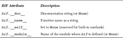
You can list all attributes of a function by using dir():

Internally, BIFs are represented as the same type as built-in methods (BIMs), so invoking type() on a BIF or BIM results in:
>>> type(dir)
<type 'builtin_function_or_method'>
Note that this does not apply to factory functions, where type() correctly returns the type of object produced:

UDFs are generally written in Python and defined at the top-level part of a module and hence are loaded as part of the global namespace (once the built-in namespace has been established). Functions may also be defined in other functions, and due to the nested scopes improvement in 2.2, we now have access to attributes in multiply-nested scopes. Hooks to attributes defined elsewhere are provided by the func_closure attribute.
Like the BIFs above, UDFs also have many attributes. The more interesting and specific ones to UDFs are listed below in Table 14.2.
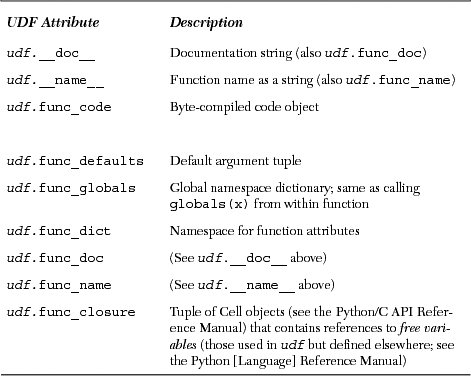
Internally, user-defined functions are of the type “function,” as indicated in the following example by using type():
![]()
Lambda expressions are the same as user-defined functions with some minor differences. Although they yield function objects, lambda expressions are not created with the def statement and instead are created using the lambda keyword.
Because lambda expressions do not provide the infrastructure for naming the codes that are tied to them, lambda expressions must be called either through functional programming interfaces or have their reference be assigned to a variable, and then they can be invoked directly or again via functional programming. This variable is merely an alias and is not the function object’s name.
Function objects created by lambda also share all the same attributes as user-defined functions, with the only exception resulting from the fact that they are not named; the __name__ or func_name attribute is given the string “<lambda>”.
Using the type() factory function, we show that lambda expressions yield the same function objects as user-defined functions:
In the example above, we assign the expression to an alias. We can also invoke type() directly on a lambda expression:
>>> type(lambda:1)
<type 'function'>
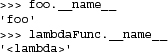
Let us take a quick look at UDF names, using lambdaFunc above and foo from the preceding subsection:
As we noted back in Section 11.9, programmers can also define function attributes once the function has been declared (and a function object available). All of the new attributes become part of the udf.__dict__ object. Later on in this chapter, we will discuss taking strings of Python code and executing it. There will be a combined example toward the end of the chapter highlighting function attributes and dynamic evaluation of Python code (from strings) and executing those statements.
In Chapter 13 we discovered methods, functions that are defined as part of a class—these are user-defined methods. Many Python data types such as lists and dictionaries also have methods, known as built-in methods. To further show this type of “ownership,” methods are named with or represented alongside the object’s name via the dotted-attribute notation.
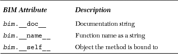
We discussed in the previous section how built-in methods are similar to built-in functions. Only built–in types (BITs) have BIMs. As you can see below, the type() factory function gives the same output for built-in methods as it does for BIFs—note how we have to provide a built-in type (object or reference) in order to access a BIM:
>>> type([].append)
<type 'builtin_function_or_method'>
Furthermore, both BIMs and BIFs share the same attributes, too. The only exception is that now the __self__ attribute points to a Python object (for BIMs) as opposed to None (for BIFs):
Recall that for classes and instances, their data and method attributes can be obtained by using the dir() BIF with that object as the argument to dir(). It can also be used with BIMs:

It does not take too long to discover, however, that using an actual object to access its methods does not prove very useful functionally, as in the last example. No reference is saved to the object, so it is immediately garbage-collected. The only thing useful you can do with this type of access is to use it to display what methods (or members) a BIT has.
User-defined methods are contained in class definitions and are merely “wrappers” around standard functions, applicable only to the class they are defined for. They may also be called by subclass instances if not overridden in the subclass definition.
As explained in Chapter 13, UDMs are associated with class objects (unbound methods), but can be invoked only with class instances (bound methods). Regardless of whether they are bound or not, all UDMs are of the same type, “instance method,” as seen in the following calls to type():

UDMs have attributes as shown in Table 14.4.

Accessing the object itself will reveal whether you are referring to a bound or an unbound method. As you can also see below, a bound method reveals to which instance object a method is bound:

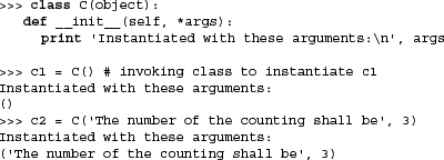
The callable property of classes allows instances to be created. “Invoking” a class has the effect of creating an instance, better known as instantiation. Classes have default constructors that perform no action, basically consisting of a pass statement. The programmer may choose to customize the instantiation process by implementing an __init__() method. Any arguments to an instantiation call are passed on to the constructor:
We are already familiar with the instantiation process and how it is accomplished, so we will keep this section brief. What is new, however, is how to make instances callable.
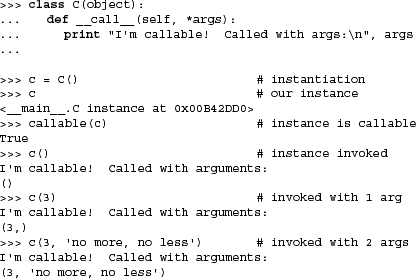
Python provides the __call__() special method for classes, which allows a programmer to create objects (instances) that are callable. By default, the __call__() method is not implemented, meaning that most instances are not callable. However, if this method is overridden in a class definition, instances of such a class are made callable. Calling such instance objects is equivalent to invoking the __call__() method. Naturally, any arguments given in the instance call are passed as arguments to __call__().
You also have to keep in mind that __call__() is still a method, so the instance object itself is passed in as the first argument to __call__() as self. In other words, if foo is an instance, then foo() has the same effect as foo.__call__(foo)—the occurrence of foo as an argument—simply the reference to self that is automatically part of every method call. If __call__() has arguments, i.e., __call__(self,arg), then foo(arg) is the same as invoking foo.__call__(foo,arg). Here we present an example of a callable instance, using a similar example as in the previous section:
We close this subsection with a note that class instances cannot be made callable unless the __call__() method is implemented as part of the class definition.
Callables are a crucial part of the Python execution environment, yet they are only one element of a larger landscape. The grander picture consists of Python statements, assignments, expressions, and even modules. These other “executable objects” do not have the ability to be invoked like callables. Rather, these objects are the smaller pieces of the puzzle that make up executable blocks of code called code objects.
At the heart of every callable is a code object, which consists of statements, assignments, expressions, and other callables. Looking at a module means viewing one large code object that contains all the code found in the module. Then it can be dissected into statements, assignments, expressions, and callables, which recurse to another layer as they contain their own code objects.
In general, code objects can be executed as part of function or method invocations or using either the exec statement or eval() BIF. A bird’s eye view of a Python module also reveals a single code object representing all lines of code that make up that module.
If any Python code is to be executed, that code must first be converted to byte-compiled code (aka bytecode). This is precisely what code objects are.
They do not contain any information about their execution environment, however, and that is why callables exist, to “wrap” a code object and provide that extra information.
Recall, from the previous section, the udf.func_code attribute for a UDFs? Well, guess what? That is a code object. Or how about the udm.im_func function object for UDMs? Since that is also a function object, it also has its own udm.im_func.func_code code object. So you can see that function objects are merely wrappers for code objects, and methods are wrappers for function objects. You can start anywhere and dig. When you get to the bottom, you will have arrived at a code object.
Python provides a number of BIFs supporting callables and executable objects, including the exec statement. These functions let the programmer execute code objects as well as generate them using the compile() BIF. They are listed in Table 14.5.
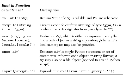
callable() is a Boolean function that determines if an object type can be invoked via the function operator ( ( ) ). It returns True if the object is callable and False otherwise (1 and 0, respectively, for Python 2.2 and earlier). Here are some sample objects and what callable returns for each type:

compile() is a function that allows the programmer to generate a code object on the fly, that is, during runtime. These objects can then be executed or evaluated using the exec statement or eval() BIF. It is important to bring up the point that both exec and eval() can take string representations of Python code to execute. When executing code given as strings, the process of byte-compiling such code must occur every time. The compile() function provides a one-time byte-code compilation of code so that the precompile does not have to take place with each invocation. Naturally, this is an advantage only if the same pieces of code are executed more than once. In these cases, it is definitely better to precompile the code.
All three arguments to compile() are required, with the first being a string representing the Python code to compile. The second string, although required, is usually set to the empty string. This parameter represents the file name (as a string) where this code object is located or can be found. Normal usage is for compile() to generate a code object from a dynamically generated string of Python code—code that obviously does not originate from an existing file.
The last argument is a string indicating the code object type. There are three possible values:
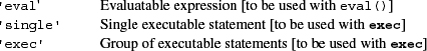
>>> single_code = compile('print "Hello world!"', '', 'single')
>>> single_code
<code object ? at 120998, file "", line 0>
>>> exec single_code
Hello world!
In the final example, we see input() for the first time. Since the beginning, we have been reading input from the user using raw_input(). The input() BIF is a shortcut function that we will discuss later in this chapter. We just wanted to tease you with a sneak preview.
eval() evaluates an expression, either as a string representation or a pre-compiled code object created via the compile() built-in. This is the first and most important argument to eval()... it is what you want to execute.
The second and third parameters, both optional, represent the objects in the global and local namespaces, respectively. If provided, globals must be a dictionary. If provided, locals can be any mapping object, e.g., one that implements the __getitem__() special method. (Before 2.4, locals was required to be a dictionary.) If neither of these are given, they default to objects returned by globals() and locals(), respectively. If only a globals dictionary is passed in, then it is also passed in as locals.
Okay, now let us take a look at eval():

We see that in this case, both eval() and int() yield the same result: an integer with the value 932. The paths they take are somewhat different, however. The eval() BIF takes the string in quotes and evaluates it as a Python expression. The int() BIF takes a string representation of an integer and converts it to an integer. It just so happens that the string consists exactly of the string 932, which as an expression yields the value 932, and that 932 is also the integer represented by the string “932.” Things are not the same, however, when we use a pure string expression:
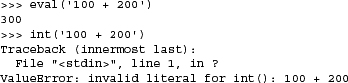
In this case, eval() takes the string and evaluates "100 + 200" as an expression, which, after performing integer addition, yields the value 300. The call to int() fails because the string argument is not a string representation of an integer—there are invalid literals in the string, namely, the spaces and “+” character.
One simple way to envision how the eval() function works is to imagine that the quotation marks around the expression are invisible and think, “If I were the Python interpreter, how would I view this expression?” In other words, how would the interpreter react if the same expression were entered interactively? The output after pressing the RETURN or ENTER key should be the same as what eval() will yield.
Like eval(), the exec statement also executes either a code object or a string representing Python code. Similarly, precompiling oft-repeated code with compile() helps improve performance by not having to go through the byte-code compilation process for each invocation. The exec statement takes exactly one argument, as indicated here with its general syntax:
execobj
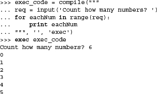
The executed object (obj) can be either a single statement or a group of statements, and either may be compiled into a code object (with “single” or “exec,” respectively) or it can be just the raw string. Below is an example of multiple statements being sent to exec as a single string:

Finally, exec can also accept a valid file object to a (valid) Python file. If we take the code in the multi-line string above and create a file called xcount.py, then we could also execute the same code with the following:
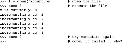
Note that once execution has completed, a successive call to exec fails. Well, it doesn’t really fail ... it just doesn’t do anything, which may have caught you by surprise. In reality, exec has read all the data in the file and is sitting at the end-of-file (EOF). When exec is called again with the same file object, there is no more code to execute, so it does not do anything, hence the behavior seen above. How do we know that it is at EOF?
We use the file object’s tell() method to tell us where we are in the file and then use os.path.getsize() to tell us how large our xcount.py script was. As you can see, there is an exact match:

If we really want to run it again without closing and reopening the file, you can just seek() to the beginning of the file and call exec again. For example, let us assume that we did not call f.close() yet. Then we can do the following:

The input() BIF is the same as the composite of eval() and raw_input(), equivalent to eval(raw_input()). Like raw_input(), input() has an optional parameter, which represents a string prompt to display to the user. If not provided, the string has a default value of the empty string.
Functionally, input() differs from raw_input() because raw_input() always returns a string containing the user’s input, verbatim. input() performs the same task of obtaining user input; however, it takes things one step further by evaluating the input as a Python expression. This means that the data returned by input() are a Python object, the result of performing the evaluation of the input expression.
One clear example is when the user inputs a list. raw_input() returns the string representation of a list, while input() returns the actual list:

The above was performed with raw_input(). As you can see, everything is a string. Now let us see what happens when we use input() instead:
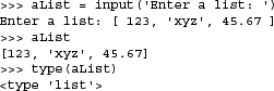
Although the user input a string, input() evaluates that input as a Python object and returns the result of that expression.
In this section, we will look at two examples of Python scripts that take Python code as strings and execute them at runtime. The first example is more dynamic, but the second shows off function attributes at the same time.
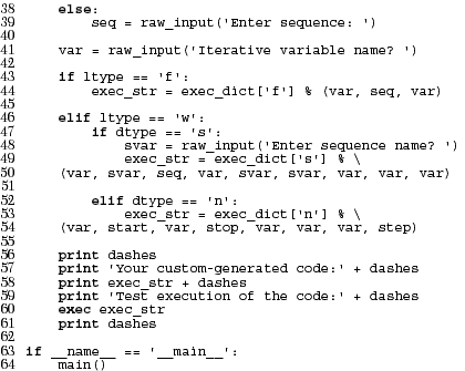
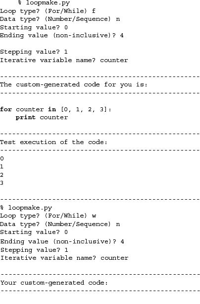
The first example is loopmake.py script, which is a simple computer-aided software engineering (CASE) that generates and executes loops on-the-fly. It prompts the user for the various parameters (i.e., loop type (while or for), type of data to iterate over [numbers or sequences]), generates the code string, and executes it.

Here are a few example executions of this script:

In this first part of the script, we are setting up two global variables. The first is a static string consisting of a line of dashes (hence the name) and the second is a dictionary of the skeleton code we will need to use for the loops we are going to generate. The keys are “f” for a for loop, “s” for a while loop iterating through a sequence, and “n” for a counting while loop.
Here we prompt the user for the type of loop he or she wants and what data types to use.
Numbers have been chosen; they provide the starting, stopping, and incremental values. In this section of code, we are introduced to the input() BIF for the first time. As we shall see in Section 14.3.5, input() is similar to raw_input() in that it prompts the user for string input, but unlike raw_input(), input() also evaluates the input as a Python expression, rendering a Python object even if the user typed it in as a string.
Output the generated source code as well as the resulting output from execution of the aforementioned generated code.
Execute main() only if this module was invoked directly.
To keep the size of this script to a manageable size, we had to trim all the comments and error checking from the original script. You can find both the original as well as an alternate version of this script on the book’s Web site.
The extended version includes extra features such as not requiring enclosing quotation marks for string input, default values for input data, and detection of invalid ranges and identifiers; it also does not permit built-in names or keywords as variable names.
Our second example highlights the usefulness of function attributes introduced back in Chapter 11, “Functions”, inspired by the example in PEP 232. Let us assume that you are a software QA developer encouraging your engineers to install either regression testers or regression instruction code into the main source but do not want the testing code mixed with the production code. You can tell your engineers to create a string representing the testing code. When your test framework executes, it checks to see if that function has defined a test body, and if so, (evaluates and) executes it. If not, it will skip and continue as normal.
Example 14.2. Function Attributes (funcAttrs.py)
Calling sys.exit() causes the Python interpreter to quit. Any integer argument to exit() will be returned to the caller as the exit status, which has a default value of 0.

We define foo() and bar() in the first part of this script. Neither function does anything other than return True. The one difference between the two is that foo() has no attributes while bar() gets a documentation string.
Using function attributes, we add a doc string and a regression or unit tester string to foo(). Note that the tester string is actually comprised of real lines of Python code.
Okay, the real work happens here. We start by iterating through the current (global) namespace using the dir() BIF. It returns a list of the object names. Since these are all strings, we need line 19 to turn them into real Python objects.
Other than the expected system variables, i.e., __builtins__, we expect our functions to show up. We are only interested in functions; the code in line 20 will let us skip any non-function objects encountered. Once we know we have a function, we check to see if it has a doc string, and if so, we display it.
Lines 23–27 perform some magic. If the function has a tester attribute, then execute it, otherwise let the user know that no unit tester is available. The last few lines display the names of non-function objects encountered.
Upon executing the script, we get the following output:

When we discuss the execution of other programs, we distinguish between Python programs and all other non-Python programs, which include binary executables or other scripting language source code. We will cover how to run other Python programs first, then how to use the os module to invoke external programs.
During runtime, there are a number of ways to execute another Python script. As we discussed earlier, importing a module the first time will cause the code at the top level of that module to execute. This is the behavior of Python importing, whether desired or not. We remind you that the only code that belongs to the top level of a module are global variables, and class and function declarations.
Core Note: All modules executed when imported

This is just a friendly reminder: As already alluded to earlier in Chapters 3 and 12, we will tell you one more time that Python modules are executed when they are imported! When you import the foo module, it runs all of the top-level (not indented) Python code, i.e., “main()”. If foo contains a declaration for the bar function, then def bar(...) is executed. Why is that again?
Well, just think what needs to be done in order for the call foo.bar() to succeed. Somehow bar has to be recognized as a valid name in the foo module (and in foo ’s namespace), and second, the interpreter needs to know it is a declared function, just like any other function in your local module.
Now that we know what we need to do, what do we do with code that we do not want executed every time our module is imported? Indent it and put it in the suite for the if __name__ == '__main__'.
These should be followed by an if statement that checks __name__ to determine if a script is invoked, i.e., “if__name__ == '__main__'”. In these cases, your script can then execute the main body of code, or, if this script was meant to be imported, it can run a test suite for the code in this module.
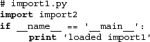
One complication arises when the imported module itself contains import statements. If the modules in these import statements have not been loaded yet, they will be loaded and their top-level code executed, resulting in recursive import behavior. We present a simple example below. We have two modules import1 and import2, both with print statements at their outermost level. import1 imports import2 so that when we import import1 from within Python, it imports and “executes” import2 as well.
Here are the contents of import1.py:
And here are the contents of import2.py:
# import2.py
print 'loaded import2'
Here is the output when we import import1 from Python:

Following our suggested workaround of checking the value of __name__, we can change the code in import1.py and import2.py so that this behavior does not occur.
Here is the modified version of import1.py:
The following is the code for import2.py, changed in the same manner:
![]()
We no longer get any output when we import import1 from Python:
>>> import import1
>>>
Now it does not necessarily mean that this is the behavior you should code for all situations. There may be cases where you want to display output to confirm a module import. It all depends on your situation. Our goal is to provide pragmatic programming examples to prevent unintended side effects.
It should seem apparent that importing a module is not the preferred method of executing a Python script from within another Python script; that is not what the importing process is. One side effect of importing a module is the execution of the top-level code.
Earlier in this chapter, we described how the exec statement can be used with a file object argument to read the contents of a Python script and execute it. This can be accomplished with the following code segment:
![]()
The three lines can be replaced by a single call to execfile():
execfile(filename)
Although the code above does execute a module, it does so only in its current execution environment (i.e., its global and local namespace). There may be a desire to execute a module with a different set of global and local namespaces instead of the default ones. The full syntax of execfile() is very similar to that of eval():
execfile(filename, globals=globals(), locals=locals())
Like eval(), both globals and locals are optional and default to the executing environments’ namespaces if not given. If only globals is given, then locals defaults to globals. If provided, locals can be any mapping object [an object defining/overriding __getitem__()], although before 2.4, it was required to be a dictionary. Warning: be very careful with your local namespace (in terms of modifying it). It is much safer to pass in a dummy “locals” dictionary and check for any side effects. Altering the local namespace is not guaranteed by execfile()! See the Python Library Reference Manual’s entry for execfile() for more details.
A new command-line option (or switch) was added in Python 2.4 that allows you to directly execute a module as a script from your shell or DOS prompt. When you are writing your own modules as scripts, it is easy to execute them. From your working directory, you would just call your script on the command line:
$ myScript.py # or $ python myScript.py
This is not as easy if you are dealing with modules that are part of the standard library, installed in site-packages, or just modules in packages, especially if they also share the same name as an existing Python module. For example, let us say you wanted to run the free Web server that comes with Python so that you can create and test Web pages and CGI scripts you wrote.
You would have to type something like the following at the command line:
$ python /usr/local/lib/python2x/CGIHTTPServer.py
Serving HTTP on 0.0.0.0 port 8000 ...
That is a long line to type, and if it is a third-party, you would have to dig into site-packages to find exactly where it is located, etc. Can we run a module from the command line without the full pathname and let Python’s import mechanism do the legwork for us?
That answer is yes. We can use the Python -c command-line switch:
$ python -c "import CGIHTTPServer; CGIHTTPServer.test()"
This option allows you to specify a Python statement you wish to run. So it does work, but the problem is that the __name__ module is not '__main__'... it is whatever module name you are using. (You can refer back to Section 3.4.1 for a review of __name__ if you need to.) The bottom line is that the interpreter has loaded your module by import and not as a script. Because of this, all of the code under if __name__=='__main__' will not execute, so you have to do it manually like we did above calling the test() function of the module.
So what we really want is the best of both worlds—being able to execute a module in your library but as a script and not as an imported module. That is the main motivation behind the -m option. Now you can run a script like this:
$ python -m CGIHTTPServer
That is quite an improvement. Still, the feature was not as fully complete as some would have liked. So in Python 2.5, the -m switch was given even more capability. Starting with 2.5, you can use the same option to run modules inside packages or modules that need special loading, such as those inside ZIP files, a feature added in 2.3 (see Section 12.5.7 on page 396). Python 2.4 only lets you execute standard library modules. So running special modules like PyChecker (Python’s “lint”), the debugger (pdb), or any of the profilers (note that these are modules that load and run other modules) was not solved with the initial -m solution but is fixed in 2.5.
We can also execute non-Python programs from within Python. These include binary executables, other shell scripts, etc. All that is required is a valid execution environment, i.e., permissions for file access and execution must be granted, shell scripts must be able to access their interpreter (Perl, bash, etc.), binaries must be accessible (and be of the local machine’s architecture).
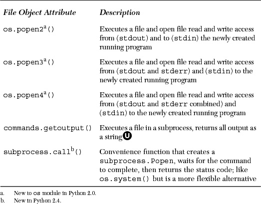
Finally, the programmer must bear in mind whether our Python script is required to communicate with the other program that is to be executed. Some programs require input, others return output as well as an error code upon completion (or both). Depending on the circumstances, Python provides a variety of ways to execute non-Python programs. All of the functions discussed in this section can be found in the os module. We provide a summary for you in Table 14.6 (where appropriate, we annotate those that are available only for certain platforms) as an introduction to the remainder of this section.

As we get closer to the operating system layer of software, you will notice that the consistency of executing programs, even Python scripts, across platforms starts to get a little dicey. We mentioned above that the functions described in this section are in the os module. Truth is, there are multiple os modules. For example, the one for Unix-based systems (i.e., Linux, MacOS X, Solaris, *BSD, etc.) is the posix module. The one for Windows is nt (regardless of which version of Windows you are running; DOS users get the dos module), and the one for old MacOS is the mac module. Do not worry, Python will load the correct module when you call import os. You should never need to import a specific operating system module directly.
Before we take a look at each of these module functions, we want to point out for those of you using Python 2.4 and newer, there is a subprocess module that pretty much can substitute for all of these functions. We will show you later on in this chapter how to use some of these functions, then at the end give the equivalent using the subprocess.Popen class and subprocess.call() function.
The first function on our list is system(), a rather simplistic function that takes a system command as a string name and executes it. Python execution is suspended while the command is being executed. When execution has completed, the exit status will be given as the return value from system() and Python execution resumes.
system() preserves the current standard files, including standard output, meaning that executing any program or command displaying output will be passed on to standard output. Be cautious here because certain applications such as common gateway interface (CGI) programs will cause Web browser errors if output other than valid Hypertext Markup Language (HTML) strings are sent back to the client via standard output. system() is generally used with commands producing no output, some of which include programs to compress or convert files, mount disks to the system, or any other command to perform a specific task that indicates success or failure via its exit status rather than communicating via input and/or output. The convention adopted is an exit status of 0 indicating success and non-zero for some sort of failure.
For the purpose of providing an example, we will execute two commands that do have program output from the interactive interpreter so that you can observe how system() works.
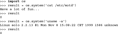
You will notice the output of both commands as well as the exit status of their execution, which we saved in the result variable. Here is an example executing a DOS command:

The popen() function is a combination of a file object and the system() function. It works in the same way as system() does, but in addition, it has the ability to establish a one-way connection to that program and then to access it like a file. If the program requires input, then you would call popen() with a mode of 'w' to “write” to that command. The data that you send to the program will then be received through its standard input. Likewise, a mode of 'r' will allow you to spawn a command, then as it writes to standard output, you can read that through your file-like handle using the familiar read*() methods of file object. And just like for files, you will be a good citizen and close() the connection when you are finished.
In one of the system() examples we used above, we called the Unix uname program to give us some information about the machine and operating system we are using. That command produced a line of output that went directly to the screen. If we wanted to read that string into a variable and perform internal manipulation or store that string to a log file, we could, using popen(). In fact, the code would look like the following:
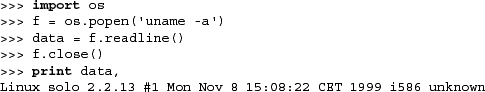
As you can see, popen() returns a file-like object; also notice that readline(), as always, preserves the NEWLINE character found at the end of a line of input text.
Without a detailed introduction to operating systems theory, we present a light introduction to processes in this section. fork() takes your single executing flow of control known as a process and creates a “fork in the road,” if you will. The interesting thing is that your system takes both forks—meaning that you will have two consecutive and parallel running programs (running the same code no less because both processes resume at the next line of code immediately succeeding the fork() call).
The original process that called fork() is called the parent process, and the new process created as a result of the call is known as the child process. When the child process returns, its return value is always zero; when the parent process returns, its return value is always the process identifier (aka process ID, or PID) of the child process (so the parent can keep tabs on all its children). The PIDs are the only way to tell them apart, too!
We mentioned that both processes will resume immediately after the call to fork(). Because the code is the same, we are looking at identical execution if no other action is taken at this time. This is usually not the intention. The main purpose for creating another process is to run another program, so we need to take divergent action as soon as parent and child return. As we stated above, the PIDs differ, so this is how we tell them apart.
The following snippet of code will look familiar to those who have experience managing processes. However, if you are new, it may be difficult to see how it works at first, but once you get it, you get it.
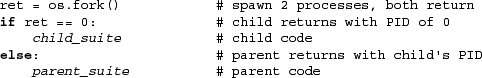
The call to fork() is made in the first line of code. Now both child and parent processes exist running simultaneously. The child process has its own copy of the virtual memory address space and contains an exact replica of the parent’s address space—yes, both processes are nearly identical. Recall that fork() returns twice, meaning that both the parent and the child return. You might ask, how can you tell them apart if they both return? When the parent returns, it comes back with the PID of the child process. When the child returns, it has a return value of 0. This is how we can differentiate the two processes.
Using an if-else statement, we can direct code for the child to execute (i.e., the if clause) as well as the parent (the else clause). The code for the child is where we can make a call to any of the exec*() functions to run a completely different program or some function in the same program (as long as both child and parent take divergent paths of execution). The general convention is to let the children do all the dirty work while the parent either waits patiently for the child to complete its task or continues execution and checks later to see if the child finished properly.
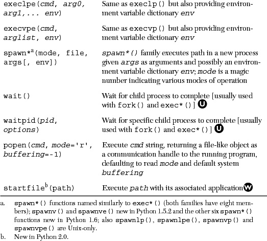
All of the exec*() functions load a file or command and execute it with an argument list (either individually given or as part of an argument list). If applicable, an environment variable dictionary can be provided for the command. These variables are generally made available to programs to provide a more accurate description of the user’s current execution environment. Some of the more well-known variables include the user name, search path, current shell, terminal type, localized language, machine type, operating system name, etc.
All versions of exec*() will replace the Python interpreter running in the current (child) process with the given file as the program to execute now. Unlike system(), there is no return to Python (since Python was replaced). An exception will be raised if exec*() fails because the program cannot execute for some reason.
The following code starts up a cute little game called “xbill” in the child process while the parent continues running the Python interpreter. Because the child process never returns, we do not have to worry about any code for the child after calling exec*(). Note that the command is also a required first argument of the argument list.

In this code, you also find a call to wait(). When children processes have completed, they need their parents to clean up after them. This task, known as “reaping a child,” can be accomplished with the wait*() functions. Immediately following a fork(), a parent can wait for the child to complete and do the clean-up then and there. A parent can also continue processing and reap the child later, also using one of the wait*() functions.
Regardless of which method a parent chooses, it must be performed. When a child has finished execution but has not been reaped yet, it enters a limbo state and becomes known as a zombie process. It is a good idea to minimize the number of zombie processes in your system because children in this state retain all the system resources allocated in their lifetimes, which do not get freed or released until they have been reaped by the parent.
A call to wait() suspends execution (i.e., waits) until a child process (any child process) has completed, terminating either normally or via a signal. wait() will then reap the child, releasing any resources. If the child has already completed, then wait() just performs the reaping procedure. waitpid() performs the same functionality as wait() with the additional arguments’ PID to specify the process identifier of a specific child process to wait for plus options (normally zero or a set of optional flags logically OR’d together).
The spawn*() family of functions are similar to fork() and exec*() in that they execute a command in a new process; however, you do not need to call two separate functions to create a new process and cause it to execute a command. You only need to make one call with the spawn*() family. With its simplicity, you give up the ability to “track” the execution of the parent and child processes; its model is more similar to that of starting a function in a thread. Another difference is that you have to know the magic mode parameter to pass to spawn*().
On some operating systems (especially embedded real-time operating systems [RTOs]), spawn*() is much faster than fork(). (Those where this is not the case usually use copy-on-write tricks.) Refer to the Python Library Reference Manual for more details (see the Process Management section of the manual on the os module) on the spawn*() functions. Various members of the spawn*() family were added to Python between 1.5 and 1.6 (inclusive).
After Python 2.3 came out, work was begun on a module named popen5. The naming continued the tradition of all the previous popen*() functions that came before, but rather than continuing this ominous trend, the module was eventually named subprocess, with a class named Popen that has functionality to centralize most of the process-oriented functions we have discussed so far in this chapter. There is also a convenience function named call() that can easily slide into where os.system() lives. The subprocess module made its debut in Python 2.4. Below is an example of what it can do:
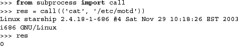


Table 14.7 lists some of the functions (and their modules) that can perform some of the tasks described.
At one time in Python’s history, there was the concept of restricted execution using the rexec and Bastion modules. The first allowed you to modify the built-in objects that were made available to code executing in a sandbox. The second served as an attribute filter and wrapper around your classes. However, due to a well-known vulnerability and the difficulty in fixing the security hole, these modules are no longer used or accessible; their documentation serves only those maintaining old code using these modules.
Clean execution occurs when a program runs to completion, where all statements in the top level of your module finish execution and your program exits. There may be cases where you may want to exit from Python sooner, such as a fatal error of some sort. Another case is when conditions are not sufficient to continue execution.
In Python, there are varying ways to respond to errors. One is via exceptions and exception handling. Another way is to construct a “cleaner” approach so that the main portions of code are cordoned off with if statements to execute only in non-error situations, thus letting error scenarios terminate “normally.” However, you may also desire to exit the calling program with an error code to indicate that such an event has occurred.
The primary way to exit a program immediately and return to the calling program is the exit() function found in the sys module. The syntax for sys.exit() is:
sys.exit(status=0)
When sys.exit() is called, a SystemExit exception is raised. Unless monitored (in a try statement with an appropriate except clause), this exception is generally not caught or handled, and the interpreter exits with the given status argument, which defaults to zero if not provided. SystemExit is the only exception that is not viewed as an error. It simply indicates the desire to exit Python.
One popular place to use sys.exit() is after an error is discovered in the way a command was invoked, in particular, if the arguments are incorrect, invalid, or if there are an incorrect number of them. The following Example 14.3 (args.py) is just a test script we created to require that a certain number of arguments be given to the program before it can execute properly.
Executing this script we get the following output:

Example 14.4. Exiting Immediately (args.py)
Calling sys.exit() causes the Python interpreter to quit. Any integer argument to exit() will be returned to the caller as the exit status, which has a default value of 0.

Many command-line-driven programs test the validity of the input before proceeding with the core functionality of the script. If the validation fails at any point, a call is made to a usage() function to inform the user what problem caused the error as well as a usage “hint” to aid the user so that he or she will invoke the script properly the next time.
sys.exitfunc() is disabled by default, but can be overridden to provide additional functionality, which takes place when sys.exit() is called and before the interpreter exits. This function will not be passed any arguments, so you should create your function to take no arguments.
If sys.exitfunc has already been overridden by a previously defined exit function, it is good practice to also execute that code as part of your exit function. Generally, exit functions are used to perform some type of shutdown activity, such as closing a file or network connection, and it is always a good idea to complete these maintenance tasks, such as releasing previously held system resources.
Here is an example of how to set up an exit function, being sure to execute one if one has already been set:

We execute the old exit function after our cleanup has been performed. The getattr() call simply checks to see whether a previous exitfunc has been defined. If not, then None is assigned to prev_exit_func; otherwise, prev_exit_func becomes a new alias to the exiting function, which is then passed as a default argument to our new exit function, my_exit_func.
The call to getattr() could have been rewritten as:

The _exit() function of the os module should not be used in general practice. (It is platform-dependent and available only on certain platforms, i.e., Unix-based and Win32.) Its syntax is:
os._exit(status)
This function provides functionality opposite to that of sys.exit() and sys.exitfunc(), exiting Python immediately without performing any cleanup (Python or programmer-defined) at all. Unlike sys.exit(), the status argument is required. Exiting via sys.exit() is the preferred method of quitting the interpreter.
The kill() function of the os module performs the traditional Unix function of sending a signal to a process. The arguments to kill() are the process identification number (PID) and the signal you wish to send to that process. The typical signal that is sent is either SIGINT, SIGQUIT, or more drastically, SIGKILL, to cause a process to terminate.
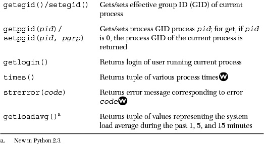
In this chapter, we have seen various ways to interact with your operating system (OS) via the os module. Most of the functions we looked at dealt with either files or external process execution. There are a few more that allow for more specific actions for the current user and process, and we will look at them briefly here. Most of the functions described in Table 14.8 work on POSIX systems only, unless also denoted for Windows environment.

In Table 14.9 you will find a list of modules other than os and sys that relate to the execution environment theme of this chapter.

14-1. Callable Objects. Name Python’s callable objects.
14-2. exec versus eval(). What is the difference between the exec statement and the eval() BIF?
14-3. input() versus raw.input(). What is the difference between the BIFs input() and raw_input()?
14-4. Execution Environment. Create a Python script that runs other Python scripts.
14-5. os.system(). Choose a familiar system command that performs a task without requiring input and either outputs to the screen or does not output at all. Use the os.system() call to run that program. Extra credit: Port your solution to subprocess.call().
14-6. commands.getoutput(). Solve the previous problem using commands.getoutput().
14-7. popen() Family. Choose another familiar system command that takes text from standard input and manipulates or otherwise outputs the data. Use os.popen() to communicate with this program. Where does the output go? Try using popen2.popen2() instead.
14-8. subprocess Module. Take your solutions from the previous problem and port them to the subprocess module.
14-9. Exit Function. Design a function to be called when your program exits. Install it as sys.exitfunc(), run your program, and show that your exit function was indeed called.
14-10. Shells. Create a shell (operating system interface) program. Present a command-line interface that accepts operating system commands for execution (any platform).
Extra credit 1: Support pipes (see the dup(), dup2(), and pipe() functions in the os module). This piping procedure allows the standard output of one process to be connected to the standard input of another.
Extra credit 2: Support inverse pipes using parentheses, giving your shell a functional programming-like interface. In other words, instead of piping commands like ...
ps -ef | grep root | sort -n +1
... support a more functional style like...
sort(grep(ps (-ef), root), -n, +1)
14-11. fork()/exec*() versus spawn*(). What is the difference between using the fork()-exec*() pairs vs. the spawn*() family of functions? Do you get more with one over the other?
14-12. Generating and Executing Python Code. Take the funcAttrs.py script (Example 14.2) and use it to add testing code to functions that you have in some of your existing programs. Build a testing framework that runs your test code every time it encounters your special function attributes.