
Chapter Topics
In this chapter, we will focus on Python’s numeric types. We will cover each type in detail, then present the various operators and built-in functions that can be used with numbers. We conclude this chapter by introducing some of the standard library modules that deal with numbers.
Numbers provide literal or scalar storage and direct access. A number is also an immutable type, meaning that changing or updating its value results in a newly allocated object. This activity is, of course, transparent to both the programmer and the user, so it should not change the way the application is developed.
Python has several numeric types: “plain” integers, long integers, Boolean, double-precision floating point real numbers, decimal floating point numbers, and complex numbers.
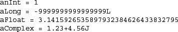
Creating numbers is as simple as assigning a value to a variable:
You can “update” an existing number by (re)assigning a variable to another number. The new value can be related to its previous value or to a completely different number altogether. We put quotes around update because you are not really changing the value of the original variable. Because numbers are immutable, you are just making a new number and reassigning the reference. Do not be fooled by what you were taught about how variables contain values that allow you to update them. Python’s object model is more specific than that.
When we learned programming, we were taught that variables act like boxes that hold values. In Python, variables act like pointers that point to boxes. For immutable types, you do not change the contents of the box, you just point your pointer at a new box. Every time you assign another number to a variable, you are creating a new object and assigning it. (This is true for all immutable types, not just numbers.)
anInt += 1
aFloat = 2.718281828
Under normal circumstances, you do not really “remove” a number; you just stop using it! If you really want to delete a reference to a number object, just use the del statement (introduced in Section 3.5.6). You can no longer use the variable name, once removed, unless you assign it to a new object; otherwise, you will cause a NameError exception to occur.
delanInt
del aLong, aFloat, aComplex
Okay, now that you have a good idea of how to create and update numbers, let us take a look at Python’s four numeric types.
Python has several types of integers. There is the Boolean type with two possible values. There are the regular or plain integers: generic vanilla integers recognized on most systems today. Python also has a long integer size; however, these far exceed the size provided by C longs. We will take a look at these types of integers, followed by a description of operators and built-in functions applicable only to Python integer types.
The Boolean type was introduced in Python 2.3. Objects of this type have two possible values, Boolean True and False. We will explore Boolean objects toward the end of this chapter in Section 5.7.1.
Prior to 2.2, Python’s integer types were limited in size to the architecture of the machine, i.e., 32- or 64-bit. Starting in 2.2, they merged with the long integer type (see sections 5.2.3 and 5.2.4), but prior to that, the act of going beyond their limit resulted in an OverflowError. Due to the integer unification, Python integers are now unsized and will not exhibit the old overflow behavior.
Integers can be represented in decimal, octal, or hexadecimal formats. Outside of base 10, you will find a leading indicator that determines what base. For octal (base 8), it is a leading "0" until Python 2.6, at which point it changes to "0o" (or "0O") but still supports the older "0", which is removed in Python 3. Hexadecimal (base 16) is represented by "0x" or "0X". Also debuting in 2.6 are a new binary (base 2) representation "0b" and its equivalent bin() factory function. Please refer to the defining PEP 3127 for more information. Here are some examples of valid integers in Python:
0o101 84 -237 0xFFFFFFFF 017 0b0110 -680 -0X92
Long integers are no longer actively being used after Python 2.2. However, because they exist in all versions of Python (1 and) 2, we will still describe what they are for you. Previously, longs were the only unsized integer type. They distinguished themselves from “normal” ints with a trailing “L” or “l”, as in 999999999L or 0xDEADBEEFBADFEEDDEAL. All ints are now longs and just called ints. Let’s go a bit more in-depth into the unification of both these integer types.
Both integer types are in the process of being unified into a single integer type. Prior to Python 2.2, plain integer operations resulted in overflow (i.e., greater than the 232 range of numbers described above), but in 2.2 or after, there are no longer such errors.

![]()
Removing the error was the first step (no overflow, right?), as well as the addition of the OverflowWarning, which is actually suppressed by default unless enabled using the -W command-line option, hence the reason why you don’t see it above, but we can prove it exists: >>> OverflowWarning <class exceptions. OverflowWarning at 0x2b6475c2b0b0>
![]()
The next step involved bit-shifting; it used to be possible to left-shift bits out of the picture (resulting in 0):
>>> 2 << 32
0
In 2.3 such an operation gives a warning, but in 2.4 the warning is gone, and the operation results in a real (long) value:


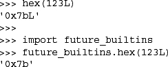
The OverflowWarning, added in 2.2 and no longer used by 2.4, was finally removed in 2.5 (see above). Python 2.6 still allows the trailing “L” syntax for longs, but the new 3.x hex() built-in function that has been backported to 2.6 via the future_builtins module no longer generates it, as shown below. You will find out more about hex() and other built-in function changes shortly.
The final phase of the unification involves removing of the long type in 3.0 as well as the trailing “L” syntax completely from the language as well as from hex() and oct().
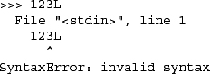
As of 2.6, there is little trace of long integers, save for the support of the trailing “L”. It is intended to serve for backwards-compatibility to allow all code which uses longs to still exist, but users should be actively purging it from their existing code and no longer using them in any new code written against 2.6+. You can read more about integer unification in PEP 237.
Floats in Python are implemented as C doubles, double precision floating point real numbers, values that can be represented in straightforward decimal or scientific notations. These 8-byte (64-bit) values conform to the IEEE 754 definition (52M/11E/1S) where 52 bits are allocated to the mantissa, 11 bits to the exponent (this gives you about ± 10308.25 in range), and the final bit to the sign. That all sounds fine and dandy; however, the actual degree of precision you will receive (along with the range and overflow handling) depends completely on the architecture of the machine as well as the implementation of the compiler that built your Python interpreter.
Floating point values are denoted by a decimal point ( . ) in the appropriate place and an optional “e” suffix representing scientific notation. We can use either lowercase ( e ) or uppercase ( E ). Positive (+) or negative ( - ) signs between the “e” and the exponent indicate the sign of the exponent. Absence of such a sign indicates a positive exponent. Here are some floating point values:
![]()
A long time ago, mathematicians were absorbed by the following equation:
x2 = -1
The reason for this is that any real number (positive or negative) multiplied by itself results in a positive number. How can you multiply any number with itself to get a negative number? No such real number exists. So in the eighteenth century, mathematicians invented something called an imaginary number i (or j, depending on what math book you are reading) such that:
Basically a new branch of mathematics was created around this special number (or concept), and now imaginary numbers are used in numerical and mathematical applications. Combining a real number with an imaginary number forms a single entity known as a complex number. A complex number is any ordered pair of floating point real numbers (x, y) denoted by x + yj where x is the real part and y is the imaginary part of a complex number.
It turns out that complex numbers are used a lot in everyday math, engineering, electronics, etc. Because it became clear that many researchers were reinventing this wheel quite often, complex numbers became a real Python data type long ago in version 1.4.
Here are some facts about Python’s support of complex numbers:
• Imaginary numbers by themselves are not supported in Python (they are paired with a real part of 0.0 to make a complex number)
• Complex numbers are made up of real and imaginary parts
• Syntax for a complex number: real+imagj
• Both real and imaginary components are floating point values
• Imaginary part is suffixed with letter “J” lowercase (j) or uppercase (J)
The following are examples of complex numbers:
![]()
Complex numbers are one example of objects with data attributes (Section 4.1.1). The data attributes are the real and imaginary components of the complex number object they belong to. Complex numbers also have a method attribute that can be invoked, returning the complex conjugate of the object.

Table 5.1 describes the attributes of complex numbers.

Numeric types support a wide variety of operators, ranging from the standard type of operators to operators created specifically for numbers, and even some that apply to integer types only.
It may be hard to remember, but when you added a pair of numbers in the past, what was important was that you got your numbers correct. Addition using the plus ( + ) sign was always the same. In programming languages, this may not be as straightforward because there are different types of numbers.
When you add a pair of integers, the + represents integer addition, and when you add a pair of floating point numbers, the + represents double-precision floating point addition, and so on. Our little description extends even to nonnumeric types in Python. For example, the + operator for strings represents concatenation, not addition, but it uses the same operator! The point is that for each data type that supports the + operator, there are different pieces of functionality to “make it all work,” embodying the concept of overloading.
Now, we cannot add a number and a string, but Python does support mixed mode operations strictly between numeric types. When adding an integer and a float, a choice has to be made as to whether integer or floating point addition is used. There is no hybrid operation. Python solves this problem using something called numeric coercion. This is the process whereby one of the operands is converted to the same type as the other before the operation. Python performs this coercion by following some basic rules.
To begin with, if both numbers are the same type, no conversion is necessary. When both types are different, a search takes place to see whether one number can be converted to the other’s type. If so, the operation occurs and both numbers are returned, one having been converted. There are rules that must be followed since certain conversions are impossible, such as turning a float into an integer, or converting a complex number to any non-complex number type.
Coercions that are possible, however, include turning an integer into a float (just add “.0”) or converting any non-complex type to a complex number (just add a zero imaginary component, e.g., “0j”). The rules of coercion follow from these two examples: integers move toward float, and all move toward complex. The Python Language Reference Guide describes the coerce() operation in the following manner.
• If either argument is a complex number, the other is converted to complex;
• Otherwise, if either argument is a floating point number, the other is converted to floating point;
• Otherwise, if either argument is a long, the other is converted to long;
• Otherwise, both must be plain integers and no conversion is necessary (in the upcoming diagram, this describes the rightmost arrow).
The flowchart shown in Figure 5-1 illustrates these coercion rules.

Automatic numeric coercion makes life easier for the programmer because he or she does not have to worry about adding coercion code to his or her application. If explicit coercion is desired, Python does provide the coerce() built-in function (described later in Section 5.6.2).
The following is an example showing you Python’s automatic coercion. In order to add the numbers (one integer, one float), both need to be converted to the same type. Since float is the superset, the integer is coerced to a float before the operation happens, leaving the result as a float:
>>> 1 + 4.5
5.5
The standard type operators discussed in Chapter 4 all work as advertised for numeric types. Mixed-mode operations, described above, are those which involve two numbers of different types. The values are internally converted to the same type before the operation is applied.
Here are some examples of the standard type operators in action with numbers:

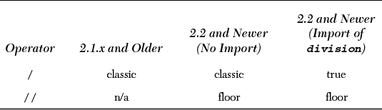
Python supports unary operators for no change and negation, + and -, respectively; and binary arithmetic operators +, -, *, /, %, and **, for addition, subtraction, multiplication, division, modulo, and exponentiation, respectively. In addition, there is a new division operator, //, as of Python 2.2.
Those of you coming from the C world are intimately familiar with classic division—that is, for integer operands, floor division is performed, while for floating point numbers, real or true division is the operation. However, for those who are learning programming for the first time, or for those who rely on accurate calculations, code must be tweaked in a way to obtain the desired results. This includes casting or converting all values to floats before performing the division.
The decision has been made to change the division operator in Python 3.0 from classic to true division and add another operator to perform floor division. We now summarize the various division types and show you what Python currently does in Python 2 versus what it does in Python 3.
When presented with integer operands, classic division truncates the fraction, returning an integer (floor division). Given a pair of floating-point operands, it returns the actual floating-point quotient (true division). This functionality is standard among many programming languages, including Python. Example:

This is where division always returns the actual quotient, regardless of the type of the operands. In Python 3, this is the algorithm of the division operator. To start migrating and use only true division with the division operator in Python 2, one must give the from __future__ import division directive. Once that happens, the division operator ( / ) performs only true division:

A new division operator ( // ) has been created that carries out floor division: it always truncates the fraction and rounds it to the next smallest whole number toward the left on the number line, regardless of the operands’ numeric types. This operator works starting in 2.2 and does not require the __future__ directive above.

There were strong arguments for as well as against this change, with the former from those who want or need true division versus those who either do not want to change their code or feel that altering the division operation from classic division is wrong.
This change was made because of the feeling that perhaps Python’s division operator has been flawed from the beginning, especially because Python is a strong choice as a first programming language for people who aren’t used to floor division. One of van Rossum’s use cases is featured in his “What’s New in Python 2.2” talk:
![]()
As you can tell, this function may or may not work correctly and is solely dependent on at least one argument being a floating point value. As mentioned above, the only way to ensure the correct value is to cast both to floats, i.e., rate = float(distance) / float(totalTime). With the upcoming change to true division, code like the above can be left as is, and those who truly desire floor division can use the new double-slash ( // ) operator.
Yes, code breakage is a concern, and the Python team has created a set of scripts that will help you convert your code to using the new style of division. Also, for those who feel strongly either way and only want to run Python with a specific type of division, check out the -Qdivision_style option to the interpreter. An option of -Qnew will always perform true division while -Qold (currently the default) runs classic division. You can also help your users transition to new division by using -Qwarn or -Qwarnall.
More information about this big change can be found in PEP 238. You can also dig through the 2001 comp.lang.python archives for the heated debates if you are interested in the drama. Table 5.2 summarizes the division operators in the various releases of Python and the differences in operation when you import new division functionality.
Integer modulo is straightforward integer division remainder, while for float, it is the difference of the dividend and the product of the divisor and the quotient of the quantity dividend divided by the divisor rounded down to the closest integer, i.e., x - (math.floor(x/y) * y), or
For complex number modulo, take only the real component of the division result, i.e., x - (math.floor((x/y).real) * y).
The exponentiation operator has a peculiar precedence rule in its relationship with the unary operators: it binds more tightly than unary operators to its left, but less tightly than unary operators to its right. Due to this characteristic, you will find the ** operator twice in the numeric operator charts in this text. Here are some examples:

In the second case, it performs 3 to the power of 2 (3-squared) before it applies the unary negation. We need to use the parentheses around the “-3” to prevent this from happening. In the final example, we see that the unary operator binds more tightly because the operation is 1 over quantity 4 to the first power ¼1 or ¼. Although 1 / 4 can be viewed strictly as an integer operation, (beginning with 2.2) Python correctly coerces both to floats so that the operation can succeed:
>>> 4 ** -1
0.25
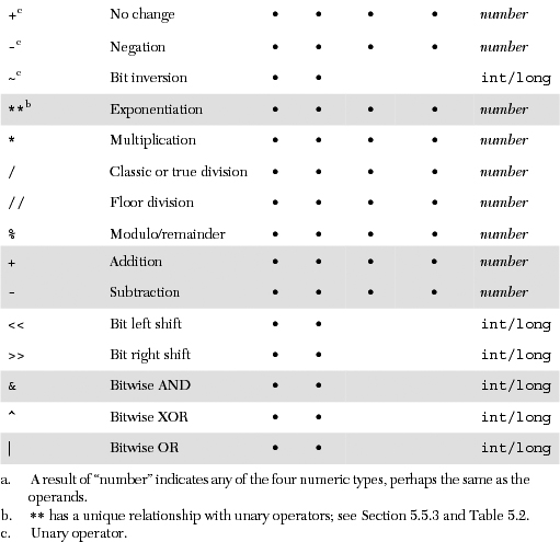
Table 5.3 summarizes all arithmetic operators, in shaded hierarchical order from highest-to-lowest priority. All the operators listed here rank higher in priority than the bitwise operators for integers found in Section 5.5.4.

Here are a few more examples of Python’s numeric operators:


Note how the exponentiation operator is still higher in priority than the binding addition operator that delimits the real and imaginary components of a complex number. Regarding the last example above, we grouped the components of the complex number together to obtain the desired result.
Python integers may be manipulated bitwise and the standard bit operations are supported: inversion, bitwise AND, OR, and exclusive OR (aka XOR), and left and right shifting. Here are some facts regarding the bit operators:
• Negative numbers are treated as their 2’s complement value.
• Left and right shifts of N bits are equivalent to multiplication and division by (2 ** N) without overflow checking.
• For longs, the bit operators use a “modified” form of 2’s complement, acting as if the sign bit were extended infinitely to the left.
The bit inversion operator ( ~ ) has the same precedence as the arithmetic unary operators, the highest of all bit operators. The bit shift operators ( << and >> ) come next, having a precedence one level below that of the standard plus and minus operators, and finally we have the bitwise AND, XOR, and OR operators (&, ^, | ), respectively. All of the bitwise operators are presented in the order of descending priority in Table 5.4.

Here we present some examples using the bit operators using 30 (011110), 45 (101101), and 60 (111100):

In the last chapter, we introduced the cmp(), str(), and type() built-in functions that apply for all standard types. For numbers, these functions will compare two numbers, convert numbers into strings, and tell you a number’s type, respectively. Here are some examples of using these functions:

Python currently supports different sets of built-in functions for numeric types. Some convert from one numeric type to another while others are more operational, performing some type of calculation on their numeric arguments.
The int(), long(), float(), and complex() functions are used to convert from any numeric type to another. Starting in Python 1.5, these functions will also take strings and return the numerical value represented by the string. Beginning in 1.6, int() and long() accepted a base parameter (see below) for proper string conversions—it does not work for numeric type conversion.
A fifth function, bool(), was added in Python 2.2. At that time, it was used to normalize Boolean values to their integer equivalents of one and zero for true and false values. The Boolean type was added in Python 2.3, so true and false now had constant values of True and False (instead of one and zero). For more information on the Boolean type, see Section 5.7.1.
In addition, because of the unification of types and classes in Python 2.2, all of these built-in functions were converted into factory functions. Factory functions, introduced in Chapter 4, just means that these objects are now classes, and when you “call” them, you are just creating an instance of that class.
They will still behave in a similar way to the new Python user so it is probably something you do not have to worry about.
The following are some examples of using these functions:

Table 5.5 summarizes the numeric type factory functions.

Python has five operational built-in functions for numeric types: abs(), coerce(), divmod(), pow(), and round(). We will take a look at each and present some usage examples.
abs() returns the absolute value of the given argument. If the argument is a complex number, then math.sqrt(num.real2 + num.imag2) is returned. Here are some examples of using the abs() built-in function:

The coerce() function, although it technically is a numeric type conversion function, does not convert to a specific type and acts more like an operator, hence our placement of it in our operational built-ins section. In Section 5.5.1, we discussed numeric coercion and how Python performs that operation. The coerce() function is a way for the programmer to explicitly coerce a pair of numbers rather than letting the interpreter do it. This feature is particularly useful when defining operations for newly created numeric class types. coerce() just returns a tuple containing the converted pair of numbers. Here are some examples:

The divmod() built-in function combines division and modulus operations into a single function call that returns the pair (quotient, remainder) as a tuple. The values returned are the same as those given for the classic division and modulus operators for integer types. For floats, the quotient returned is math.floor(num1/num2) and for complex numbers, the quotient is math.floor((num1/num2).real).

Both pow() and the double star ( ** ) operator perform exponentiation; however, there are differences other than the fact that one is an operator and the other is a built-in function.
The ** operator did not appear until Python 1.5, and the pow() built-in takes an optional third parameter, a modulus argument. If provided, pow() will perform the exponentiation first, then return the result modulo the third argument. This feature is used for cryptographic applications and has better performance than pow(x,y) % z since the latter performs the calculations in Python rather than in C-like pow(x, y, z).

The round() built-in function has a syntax of round(flt,ndig=0). It normally rounds a floating point number to the nearest integral number and returns that result (still) as a float. When the optional ndig option is given, round() will round the argument to the specific number of decimal places.

Note that the rounding performed by round() moves away from zero on the number line, i.e., round(.5) goes to 1 and round(-.5) goes to -1. Also, with functions like int(), round(), and math.floor(), all may seem like they are doing the same thing; it is possible to get them all confused. Here is how you can differentiate among these:
• int() chops off the decimal point and everything after (aka truncation).
• floor() rounds you to the next smaller integer, i.e., the next integer moving in a negative direction (toward the left on the number line).
• round() (rounded zero digits) rounds you to the nearest integer period.
Here is the output for four different values, positive and negative, and the results of running these three functions on eight different numbers. (We reconverted the result from int() back to a float so that you can visualize the results more clearly when compared to the output of the other two functions.)

Table 5.6 summarizes the operational functions for numeric types.
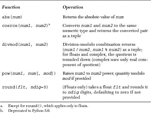
In addition to the built-in functions for all numeric types, Python supports a few that are specific only to integers (plain and long). These functions fall into two categories, base presentation with hex() and oct(), and ASCII conversion featuring chr() and ord().
As we have seen before, Python integers automatically support octal and hexadecimal representations in addition to the decimal standard. Also, Python has two built-in functions that return string representations of an integer’s octal or hexadecimal equivalent. These are the oct() and hex() built-in functions, respectively. They both take an integer (in any representation) object and return a string with the corresponding value. The following are some examples of their usage:
Python also provides functions to go back and forth between ASCII (American Standard Code for Information Interchange) characters and their ordinal integer values. Each character is mapped to a unique number in a table numbered from 0 to 255. This number does not change for all computers using the ASCII table, providing consistency and expected program behavior across different systems. chr() takes a single-byte integer value and returns a one-character string with the equivalent ASCII character. ord() does the opposite, taking a single ASCII character in the form of a string of length one and returns the corresponding ASCII value as an integer:

Table 5.7 shows all built-in functions for integer types.

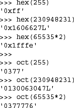
Boolean types were added to Python starting in version 2.3. Although Boolean values are spelled “True” and “False,” they are actually an integer subclass and will behave like integer values one and zero, respectively, if used in a numeric context. Here are some of the major concepts surrounding Boolean types:
• They have a constant value of either True or False.
• Booleans are subclassed from integers but cannot themselves be further derived.
• Objects that do not have a __nonzero__() method default to True.
• Recall that Python objects typically have a Boolean False value for any numeric zero or empty set.
• Also, if used in an arithmetic context, Boolean values True and False will take on their numeric equivalents of 1 and 0, respectively.
• Most of the standard library and built-in Boolean functions that previously returned integers will now return Booleans.
• Neither True nor False are keywords/constants in Python 2, but they are in Python 3.
All Python objects have an inherent True or False value. To see what they are for the built-in types, review the Core Note sidebar in Section 4.3.2. Here are some examples using Boolean values:

You can read more about Booleans in the Python documentation and PEP 285.
Decimal floating point numbers became a feature of Python in version 2.4 (see PEP 327), mainly because statements like the following drive many (scientific and financial application) programmers insane (or at least enrage them):
>>> 0.1
0.1000000000000001
Why is this? The reason is that most implementations of doubles in C are done as a 64-bit IEEE 754 number where 52 bits are allocated for the mantissa. So floating point values can only be specified to 52 bits of precision, and in situations where you have a(n endlessly) repeating fraction, expansions of such values in binary format are snipped after 52 bits, resulting in rounding errors like the above. The value .1 is represented by 0.11001100110011 ... * 2-3 because its closest binary approximation is .0001100110011 ..., or 1/16 + 1/32 + 1/256 + ...
As you can see, the fractions will continue to repeat and lead to the rounding error when the repetition cannot “be continued.” If we were to do the same thing using a decimal number, it looks much “better” to the human eye because they have exact and arbitrary precision. Note in the example below that you cannot mix and match decimals and floating point numbers. You can create decimals from strings, integers, or other decimals. You must also import the decimal module to use the Decimal number class.

You can read more about decimal numbers in the PEP as well as the Python documentation, but suffice it to say that they share pretty much the same numeric operators as the standard Python number types. Since it is a specialized numeric type, we will not include decimals in the remainder of this chapter.
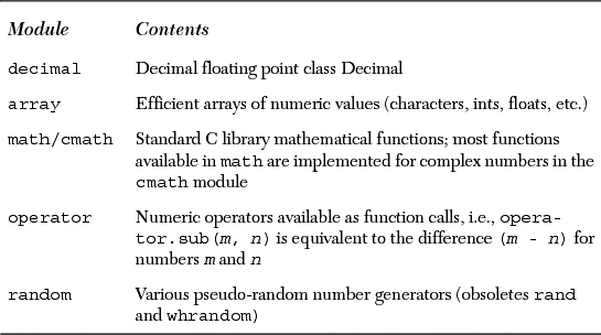
There are a number of modules in the Python standard library that add on to the functionality of the operators and built-in functions for numeric types. Table 5.8 lists the key modules for use with numeric types. Refer to the literature or online documentation for more information on these modules.
For advanced numerical and scientific mathematics applications, there are well-known third-party packages Numeric (NumPy) and SciPy, which may be of interest to you. More information on those two packages can be found at:
Core Module: random
The random module is the general-purpose place to go if you are looking for random numbers. This module comes with various pseudo-random number generators and comes seeded with the current timestamp so it is ready to go as soon as it has loaded. Here are some of the most commonly used functions in the random module:

We have now come to the conclusion of our tour of all of Python’s numeric types. A summary of operators and built-in functions for numeric types is given in Table 5.9.

The exercises in this chapter may first be implemented as applications. Once full functionality and correctness have been verified, we recommend that the reader convert his or her code to functions that can be used in future exercises. On a related note, one style suggestion is not to use print statements in functions that return a calculation. The caller can perform any output desired with the return value. This keeps the code adaptable and reusable.
5-1. Integers. Name the differences between Python’s regular and long integers.
(a) Create a function to calculate and return the product of two numbers.
(b) The code which calls this function should display the result.
5-3. Standard Type Operators. Take test score input from the user and output letter grades according to the following grade scale/curve:
A: 90-100
B: 80-89
C: 70-79
D: 60-69
E: <60
5-4. Modulus. Determine whether a given year is a leap year, using the following formula: a leap year is one that is divisible by four, but not by one hundred, unless it is also divisible by four hundred. For example, 1992, 1996, and 2000 are leap years, but 1967 and 1900 are not. The next leap year falling on a century is 2400.
5-5. Modulus. Calculate the number of basic American coins given a value less than 1 dollar. A penny is worth 1 cent, a nickel is worth 5 cents, a dime is worth 10 cents, and a quarter is worth 25 cents. It takes 100 cents to make 1 dollar. So given an amount less than 1 dollar (if using floats, convert to integers for this exercise), calculate the number of each type of coin necessary to achieve the amount, maximizing the number of larger denomination coins. For example, given $0.76, or 76 cents, the correct output would be “3 quarters and 1 penny.” Output such as “76 pennies” and “2 quarters, 2 dimes, 1 nickel, and 1 penny” are not acceptable.
5-6. Arithmetic. Create a calculator application. Write code that will take two numbers and an operator in the format: N1 OP N2, where N1 and N2 are floating point or integer values, and OP is one of the following: +, -, *, /, %, **, representing addition, subtraction, multiplication, division, modulus/remainder, and exponentiation, respectively, and displays the result of carrying out that operation on the input operands. Hint: You may use the string split() method, but you cannot use the exal() built-in function.
5-7. Sales Tax. Take a monetary amount (i.e., floating point dollar amount [or whatever currency you use]), and determine a new amount figuring all the sales taxes you must pay where you live.
5-8. Geometry. Calculate the area and volume of:
(a) squares and cubes
(b) circles and spheres
5-9. Style. Answer the following numeric format questions:
(a) Why does 17 + 32 give you 49, but 017 + 32 give you 47 and 017 + 032 give you 41, as indicated in the examples below?

(b) Why do we get 134L and not 1342 in the example below?
>>> 56l + 78l
134L
5-10. Conversion. Create a pair of functions to convert Fahrenheit to Celsius temperature values. C = (F - 32) * (5 / 9) should help you get started. We recommend you try true division with this exercise, otherwise take whatever steps are necessary to ensure accurate results.
5-11. Modulus.
(a) Using loops and numeric operators, output all even numbers from 0 to 20.
(b) Same as part (a), but output all odd numbers up to 20.
(c) From parts (a) and (b), what is an easy way to tell the difference between even and odd numbers?
(d) Using part (c), write some code to determine if one number divides another. In your solution, ask the user for both numbers and have your function answer “yes” or “no” as to whether one number divides another by returning True or False, respectively.
5-12. Limits. Determine the largest and smallest ints, floats, and complex numbers that your system can handle.
5-13. Conversion. Write a function that will take a time period measured in hours and minutes and return the total time in minutes only.
5-14. Bank Account Interest. Create a function to take an interest percentage rate for a bank account, say, a Certificate of Deposit (CD). Calculate and return the Annual Percentage Yield (APY) if the account balance was compounded daily.
5-15. GCD and LCM. Determine the greatest common divisor and least common multiple of a pair of integers.
5-16. Home Finance. Take an opening balance and a monthly payment. Using a loop, determine remaining balances for succeeding months, including the final payment. “Payment 0” should just be the opening balance and schedule monthly payment amount. The output should be in a schedule format similar to the following (the numbers used in this example are for illustrative purposes only):

5-17. *Random Numbers. Read up on the random module and do the following problem: Generate a list of a random number (1 < N <= 100) of random numbers (0 <= n <= 231-1). Then randomly select a set of these numbers (1 <= N <= 100), sort them, and display this subset.