C H A P T E R 3
Using Functions and Expressions
Now that you have the knowledge to write simple SELECT statements, it is time to explore some of the other features of T-SQL that allow you to manipulate how the data is displayed, filtered, or ordered. To create expressions in T-SQL, you use functions and operators along with literal values and columns. The reasons for using expressions in T-SQL code are many. For example, you may want to display only the year of a column of the DATETIME data type on a report, or you may need to calculate a discount based on the order quantity in an order-entry application. Any time the data must be displayed, filtered, or ordered in a way that is different from how it is stored, you can use expressions and functions to manipulate it.
You will find a very rich and versatile collection of functions and operators available to create expressions that manipulate strings and dates and much more. You can use expressions in the SELECT, WHERE, and ORDER BY clauses as well as in other clauses you will learn about in Chapter 5.
Expressions Using Operators
You learned how to use several comparison operators in the WHERE clause in Chapter 2. In this section, you will learn how to use operators to concatenate strings and perform mathematical calculations in T-SQL queries.
Concatenating Strings
The concatenation operator (+) allows you to add together two strings. The syntax is simple: <string or column name> + <string or column name>. Start up SQL Server Management Studio if it is not already running, and connect to your development server. Open a new query window, and type in and execute the code in Listing 3-1.
Listing 3-1. Concatenating Strings
USE AdventureWorks2012;

GO


--1

SELECT 'ab' + 'c';
--2

SELECT BusinessEntityID, FirstName + ' ' + LastName AS "Full Name"

FROM Person.Person;

--3

SELECT BusinessEntityID, LastName + ', ' + FirstName AS "Full Name"

FROM Person.Person;
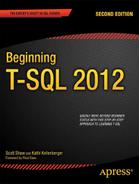
Figure 3-1 shows the results of Listing 3-1. Query 1 shows that you can concatenate two strings. Queries 2 and 3 demonstrate concatenating the LastName and FirstName columns along with either a space or a comma and space. Notice that you specified the alias, Full Name, to provide a column header for the result of the expressions combining FirstName and LastName. If you did not provide the alias, the column header would be (No column name), as in query 1.
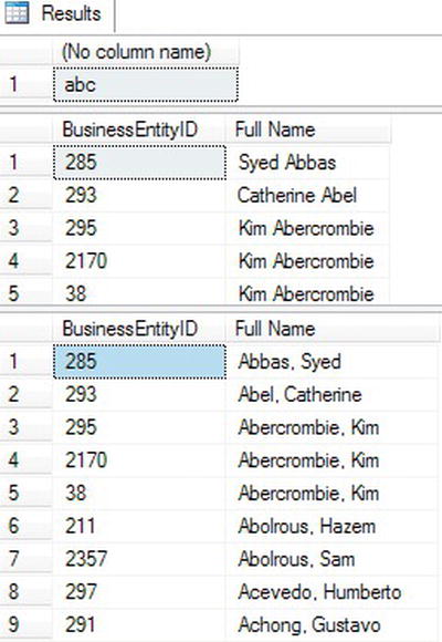
Figure 3-1. The results of queries concatenating strings
Concatenating Strings and NULL
In Chapter 2 you learned about the challenges when working with NULL in WHERE clause expressions. When concatenating a string with a NULL, NULL is returned. Listing 3-2 demonstrates this problem. Type the code in Listing 3-2 into a new query window, and execute it.
Listing 3-2. Concatenating Strings with NULL Values
USE AdventureWorks2012;

GO


SELECT BusinessEntityID, FirstName + ' ' + MiddleName +

    ' ' + LastName AS "Full Name"

FROM Person.Person;
Figure 3-2 shows the results of Listing 3-2. The query combines the FirstName, MiddleName, and LastName columns into a Full Name column. The MiddleName column is optional; that is, NULL values are allowed. Only the rows where the MiddleName value has been entered show the expected results. The rows where MiddleName is NULL return NULL.

Figure 3-2. The results of concatenating a string with NULL
CONCAT
SQL 2012 introduces another powerful tool for concatenating strings. The CONCAT statement takes any number of strings as arguments and automatically concatenates them together. The values can be passed to the CONCAT statement as variables or as regular strings. The output is always implicitly converted to a string datatype. Run the code in listing 3-3 to see how to use the CONCAT statement.
-- Simple CONCAT statement

SELECT CONCAT ('I ', 'love', ' writing', ' T-SQL') AS RESULT;


--Using variable with CONCAT

DECLARE @a VARCHAR(30) = 'My birthday is on '

DECLARE @b DATE = '08/25/1980'

SELECT CONCAT (@a, @b) AS RESULT;


--Using CONCAT with table rows

USE AdventureWorks2012

SELECT CONCAT (AddressLine1, PostalCode) AS Address

FROM Person.Address;
The first command simply concatenates four separate string values. The second example declares two variables and then concatenates those into a single result. The final example uses the CONCAT statement in a SELECT clause to concatenate table rows. Figure 3-3 shows the output. I’ve only showed the partial results for the final example.
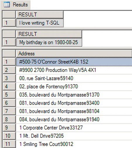
Figure 3-3. Partial Results of CONCAT Statements
ISNULL and COALESCE
Two functions are available to replace NULL values with another value. The first function, ISNULL, requires two parameters: the value to check and the replacement for NULL values. COALESCE works a bit differently. COALESCE will take any number of parameters and return the first non-NULL value. T-SQL developers often prefer COALESCE over ISNULL because COALESCE meets ANSI standards, while ISNULL does not. Also, COALESCE is more versatile. Here is the syntax for the two functions:
ISNULL(<value>,<replacement>)

COALESCE(<value1>,<value2>,...,<valueN>)
Type in and execute the code in Listing 3-4 to learn how to use ISNULL and COALESCE.
Listing 3-4. Using ISNULL and COALESCE
USE AdventureWorks2012;

GO


--1

SELECT BusinessEntityID, FirstName + ' ' + ISNULL(MiddleName,'') +

    ' ' + LastName AS "Full Name"

FROM Person.Person;

--2

SELECT BusinessEntityID, FirstName + ISNULL(' ' + MiddleName,'') +

    ' ' + LastName AS "Full Name"

FROM Person.Person;


--3

SELECT BusinessEntityID, FirstName + COALESCE(' ' + MiddleName,'') +

    ' ' + LastName AS "Full Name"

FROM Person.Person;
Figure 3-4 shows a partial result of running the code. Query 1 uses the ISNULL function to replace any missing MiddleName values with an empty string in order to build Full Name. Notice in the results that whenever MiddleName is missing, you end up with two spaces between FirstName and LastName. Line 3 in the results of query 1 contains two spaces between Kim and Ambercrombie because a space is added both before and after the ISNULL function. To correct this problem, move the space inside the ISNULL function instead of before it: ISNULL(' ' + MiddleName,''). Concatenating a space with NULL returns NULL. When the MiddleName value is NULL, the space is eliminated, and no extra spaces show up in your results. Instead of ISNULL, query 3 contains the COALESCE function. If MiddleName is NULL, the next non-NULL value, the empty string, is returned.
Figure 3-4. The results of using ISNULL and COALESCE when concatenating strings
Concatenating Other Data Types to Strings
To concatenate nonstring values to strings, the nonstring value must be converted to a string. If the string value can be implicitly converted to a number, the values will be added together instead. Run this statement to see what happens: SELECT 1 + '1';. If the desired result is 11 instead of 2, the numeric value must be converted to a string using either the CAST or CONVERT function. If you attempt to concatenate a non-numeric string and a number without converting, you will receive an error message. Run this example to see the error: SELECT 1 + 'a';.
Use one of the functions, CAST or CONVERT, to convert a numeric or temporal value to a string. Here is the syntax:
CAST(<value> AS <new data type>)

CONVERT(<new data type>,<value>)
Listing 3-5 demonstrates how to use these functions. Type in and execute the code in a query window.
Listing 3-5. Using CAST and CONVERT
USE AdventureWorks2012

GO


--1

SELECT CAST(BusinessEntityID AS NVARCHAR) + ': ' + LastName

    + ', ' + FirstName AS ID_Name

FROM Person.Person;


--2

SELECT CONVERT(NVARCHAR(10),BusinessEntityID) + ': ' + LastName

    + ', ' + FirstName AS ID_Name

FROM Person.Person;


--3

SELECT BusinessEntityID, BusinessEntityID + 1 AS "Adds 1",

    CAST(BusinessEntityID AS NVARCHAR(10)) + '1'AS "Appends 1"

FROM Person.Person;
Figure 3-5 shows the partial results of running the code. The functions in queries 1 and 2 have very different syntaxes, but they accomplish the same result.. They both change the BusinessEntityID values from integers into a string data type (NVARCHAR) so that it can be concatenated to a string. Many programmers prefer CAST over CONVERT because CAST is compliant with the ANSI SQL-99 standard. Query 1 specifies just NVARCHAR as the data type without a size. By default, the maximum length will be 30 characters. If you need to cast TO a value more than 30 characters, you must specify a length argument greater than 30. Query 3 demonstrates the difference between converting the numeric value and not converting it. For more information about CONVERT, take a look at the “CONVERT” section later in the chapter.

Figure 3-5. The partial results of using CAST and CONVERT
Developers must often concatenate strings for reports or for loading data from one system to another. Now practice what you have learned about concatenating strings within a T-SQL query by completing Exercise 3-1.
Using Mathematical Operators
You can use several operators to perform simple mathematical operations on numeric values. Use the plus symbol (+) to perform addition, the minus symbol (–) to perform subtraction, the asterisk (*) to perform multiplication, and the slash (/) to perform division. One operator that may be new to you is the modulo (%) operator. The modulo operator returns the remainder when division is performed on the two values. For example, 5 % 2 returns 1 because 1 is the remainder when you divide 5 by 2. One common use for modulo is to determine whether a number is odd or even when the second value in the expression is 2. If the result is 1, then the value is odd; if the result is 0, then the value is even. Listing 3-6 shows how to use some of the mathematical operators. Type in and execute the code to see the results.
Listing 3-6. Using Mathematical Operators
USE AdventureWorks2012;

GO


--1

SELECT 1 + 1;


--2

SELECT 10 / 3 AS DIVISION, 10 % 3 AS MODULO;


--3

SELECT OrderQty, OrderQty * 10 AS Times10

FROM Sales.SalesOrderDetail;


--4

SELECT OrderQty * UnitPrice * (1.0 - UnitPriceDiscount)

    AS Calculated, LineTotal

FROM Sales.SalesOrderDetail;


--5

SELECT SpecialOfferID,MaxQty,DiscountPct,

    DiscountPct * ISNULL(MaxQty1000) AS MaxDiscount

FROM Sales.SpecialOffer;
Take a look at the results shown in Figure 3-6. Queries 1 and 2 show how to perform calculations on literal values. Query 3 shows the result of multiplying the values stored in the OrderQty column by 10. Query 4 compares the precalculated LineTotal column to calculating the value by using an expression. The LineTotal column is a “computed column.” Computed columns have a property, PERSISTED, that allows the calculated value to be stored in the table. If the PERSISTED property of the column is set to FALSE, the value is calculated each time the data is accessed. The advantage of storing the calculated value is that you can add an index on the computed column. The actual formula used in the table definition looks a bit more complicated than the one I used since it checks for NULL values. The simplified formula I used requires parentheses to enforce the logic, causing subtraction to be performed before multiplication. Since multiplication has a higher precedence than subtraction, use parentheses to enforce the intended logic. Query 5 shows how to use the ISNULL function to substitute the value 1000 when the MaxQty is NULL before multiplying by the DiscountPct value.
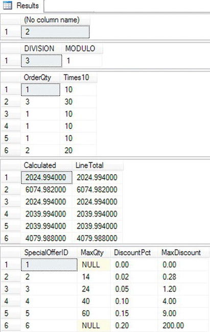
Figure 3-6. The results of using mathematical operators
Practice what you have learned about mathematical operators to complete Exercise 3-2.
Data Type Precedence
When using operators, you must keep the data types of the values in mind. When performing an operation that involves two different data types, the expression will return values with the data type with the highest precedence if possible. What value can be rolled into the other value? For example, an INT can be converted to a BIGINT, but not the other way around. In other words, if a value can be a valid INT, it is also a valid BIGINT. However, many valid BIGINT values are too big to be converted to INT. Therefore, when an operation is performed on a BIGINT and an INT, the result will be a BIGINT.
It is not always possible to convert the lower precedence data type to the higher precedence data type. A character can’t always be converted to a numeric value. For a list of possible data types in order of precedence, see the article “Data Type Precedence” in SQL Server’s help system, Books Online.
Using Functions
So far, this chapter has covered using operators along with columns and literal values to create expressions. To get around issues concerning NULL values and incompatible data types within an expression, you were introduced to several functions: ISNULL, COALESCE, CAST, and CONVERT. This section covers many other built-in functions available with SQL Server 2012.
The functions you will learn about in this chapter return a single value. The functions generally require one or more parameters. The data to be operated on can be a literal value, a column name, or the results of another function. This section covers functions to manipulate strings, dates, and numeric data. You will also learn about several system functions and how to nest one function within another function.
Using String Functions
You will find a very rich set of T-SQL functions for manipulating strings. You often have a choice of where a string will be manipulated. If the manipulation will occur on one of the columns in the select-list, it might make sense to utilize the client to do the work if the manipulation is complex, but it is possible to do quite a bit of manipulation with T-SQL. You can use the string functions to clean up data before loading it into a database. This section covers many of the commonly used string functions. You can find many more in Books Online.
RTRIM and LTRIM
The RTRIM and LTRIM functions remove spaces from the right side (RTRIM) or left side (LTRIM) of a string. You may need to use these functions when working with fixed-length data types (CHAR and NCHAR) or to clean up flat-file data before it is loaded from a staging database into a data warehouse. The syntax is simple.
RTRIM(<string>)

LTRIM(<string>)
Type in and execute the code in Listing 3-7. AdventureWorks2012The first part of the code creates and populates a temporary table. Don’t worry about understanding that part of the code at this point.
Listing 3-7. Using RTRIM and LTRIM
--Create the temp table

CREATE TABLE #trimExample (COL1 VARCHAR(10));

GO

--Populate the table

INSERT INTO #trimExample (COL1)

VALUES ('a  '),('b  '),('  c'),('  d  '),


--Select the values using the functions

SELECT COL1, '*' + RTRIM(COL1) + '*' AS "RTRIM",

    '*' + LTRIM(COL1) + '*' AS "LTRIM"

FROM #trimExample;


--Clean up

DROP TABLE #trimExample;
Figure 3-7 shows the results of the code. The INSERT statement added four rows to the table with no spaces (a), spaces on the right (b), spaces on the left (c), and spaces on both (d). Inside the SELECT statement, you will see that asterisks surround the values to make it easier to see the spaces in the results. The RTRIM function removed the spaces from the right side; the LTRIM function removed the spaces from the left side. T-SQL doesn’t contain a native function that removes the spaces from both sides of the string, but you will learn how to get around this problem in the section “Nesting Functions” later in the chapter.

Figure 3-7. The results of using RTRIM and LTRIM
LEFT and RIGHT
The LEFT and RIGHT functions return a specified number of characters on the left or right side of a string. Developers use these functions to parse strings. For example, you may need to retrieve the three-character extension from file path data by using RIGHT. Take a look at the syntax.
LEFT(<string>,<number of characters)

RIGHT(<string>,<number of characters)
Listing 3-8 demonstrates how to use these functions. Type in and execute the code.
Listing 3-8. The LEFT and RIGHT Functions
USE AdventureWorks2012;

GO

SELECT LastName,LEFT(LastName,5) AS "LEFT",

    RIGHT(LastName,4) AS "RIGHT"

FROM Person.Person

WHERE BusinessEntityID IN (293,295,211,297,299,3057,15027);
Figure 3-8 shows the results. Notice that even if the value contains fewer characters than the number specified in the second parameter, the function still works to return as many characters as possible.
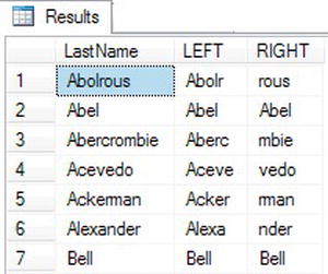
Figure 3-8. The results of using LEFT and RIGHT
LEN and DATALENGTH
Use LEN to return the number of characters in a string. Developers sometimes use another function, DATALENGTH, incorrectly in place of LEN. DATALENGTH returns the number of bytes in a string. DATALENGTH returns the same value as LEN when the string is a CHAR or VARCHAR data type, which takes one byte per character. The problem occurs when using DATALENGTH on NCHAR or NVARCHAR data types, which take two byes per characters. In this case, the DATALENGTH value is two times the LEN value. This is not incorrect; the two functions measure different things. The syntax is very simple.
LEN(<string>)

DATALENGTH(<string>)
Type in and execute the code in Listing 3-9 to learn how to use LEN and DATALENGTH.
Listing 3-9. Using the LEN and DATALENGTH Functions
USE AdventureWorks2012;

GO


SELECT LastName,LEN(LastName) AS "Length",

    DATALENGTH(LastName) AS "Data Length"

FROM Person.Person

WHERE BusinessEntityID IN (293,295,211,297,299,3057,15027);
Figure 3-9 shows the results. The Length column displays a count of the characters, while the Data Length column displays the number of bytes.

Figure 3-9. The results of using LEN and DATALENGTH
CHARINDEX
Use CHARINDEX to find the numeric starting position of a search string inside another string. By checking to see whether the value returned by CHARINDEX is greater than zero, you can use the function to just determine whether the search string exists inside the second value. Developers often use CHARINDEX to locate a particular character, such as the at symbol (@) in an e-mail address column, along with other functions when parsing strings. You will learn more about this in the “Nesting Functions” section later in the chapter. The CHARINDEX function requires two parameters: the search string and the string to be searched. An optional parameter, the start location, instructs the function to ignore a given number of characters at the beginning of the string to be searched. The following is the syntax; remember that the third parameter is optional (square brackets surround optional parameters in the syntax):
CHARINDEX(<search string>,<target string>[,<start location>])
Listing 3-10 demonstrates how to use CHARINDEX. Type in and execute the code to learn how to use this function.
Listing 3-10. Using CHARINDEX
USE AdventureWorks2012;

GO

SELECT LastName, CHARINDEX('e',LastName) AS "Find e",

    CHARINDEX('e',LastName,4) AS "Skip 4 Characters",

    CHARINDEX('be',LastName) AS "Find be",

    CHARINDEX('Be',LastName) AS "Find B"

FROM Person.Person

WHERE BusinessEntityID IN (293,295,211,297,299,3057,15027);
Figure 3-10 shows the results. The Find e column in the results displays the first location of the letter e in the LastName value. The Skip 4 Characters column displays the first location of the letter e when the first four characters of the LastName value are ignored. Finally, the Find be column demonstrates that you can use the function with search strings that are more than one character in length. Notice how “Be” returns a value of “Bell”. This is due to the case sensitivity of the AdventureWorks2012 database, which differentiates between an upper and lowercase “b.”
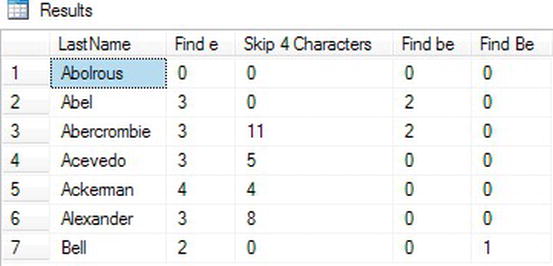
Figure 3-10. The results of using CHARINDEX
SUBSTRING
Use SUSTRING to return a portion of a string starting at a given position and for a specified number of characters. For example, an order-entry application may assign a customer ID based on the first seven letters of the customer’s last name plus digits 4–9 of the phone number. The SUBSTRING function requires three parameters: the string, a starting location, and the number of characters to retrieve. If the number of characters to retrieve is greater than the length of the string, the function will return as many characters as possible. Here is the syntax of SUBSTRING:
SUBSTRING(<string>,<start location>,<length>)
Type in and execute the code in Listing 3-11 to learn how to use SUBSTRING.
Listing 3-11. Using SUBSTRING
USE AdventureWorks2012;

GO

SELECT LastName, SUBSTRING(LastName,1,4) AS "First 4",

    SUBSTRING(LastName,5,50) AS "Characters 5 and later"

FROM Person.Person

WHERE BusinessEntityID IN (293,295,211,297,299,3057,15027);
Notice in the results (Figure 3-11) that if the starting point is located after the available characters (Abel and Bell), an empty string is returned. Otherwise, in this example, the FirstName column is divided into two strings.
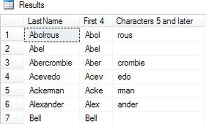
Figure 3-11. The results of using SUBSTRING
CHOOSE
CHOOSE is a new function in SQL 2012 which allows you to select a value in an array based off an index. The CHOOSE function requires an index value and list of values for the array. Here is the basic syntax for the CHOOSE function.
CHOOSE ( index, val_1, val_2 [, val_n ] )
The index simply points to the position in the array that you want to return. Listing 3-12 shows a basic example.
Listing 3-12. Using the CHOOSE Function
SELECT CHOOSE (4, 'a', 'b', c, 'd', 'e', 'f', 'g', 'h', 'i')
Figure 3-12 shows the results. Keep in mind that the results take the highest datatype precendence. This means if there is an integer in the list then the CHOOSE function will try to convert any results to an integer. If the value is a string then the CHOOSE command will throw an error. You will need to convert any interger values in the array to varchar to avoid this error.

Figure 3-12. Result from CHOOSE Function
REVERSE
REVERSE returns a string in reverse order. I often use it along with the RIGHT function to find a file name from the file’s path. I use REVERSE to find the last backslash in the path, which then tells me how many characters, minus 1, on the right side of the string I need to grab. The same method can be used to parse an e-mail address. To see how to do this, see the example in the “Nesting Functions” later in the chapter. Type in and execute this code to learn how to use REVERSE:
SELECT REVERSE('!dlroW ,olleH')
UPPER and LOWER
Use UPPER and LOWER to change a string to either uppercase or lowercase. You may need to display all uppercase data in a report, for example. The syntax is very simple.
UPPER(<string>)

LOWER(<string>)
Type in and execute the code in Listing 3-13.
Listing 3-13. Using UPPER and LOWER
USE AdventureWorks2012;

GO

SELECT LastName, UPPER(LastName) AS "UPPER",

    LOWER(LastName) AS "LOWER"

FROM Person.Person

WHERE BusinessEntityID IN (293,295,211,297,299,3057,15027);
Take a look at the results in Figure 3-13. All LastName values appear in uppercase in the UPPER column, while they appear in lowercase in the LOWER column.
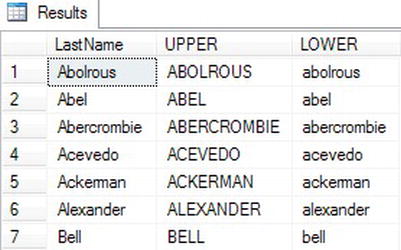
Figure 3-13. The partial results of using UPPER and LOWER
![]() Note You may think that you will use
Note You may think that you will use UPPER or LOWER often in the WHERE clause to make sure that the case of the value does not affect the results, but usually you don’t need to do this. By default, searching in T-SQL is case insensitive. The collation of the column determines whether the search will be case sensitive. This is defined at the server, but you can specify a different collation of the database, table, or column. See “Working with Collations” in Books Online for more information.
REPLACE
Use REPLACE to substitute one string value for another. REPLACE has three required parameters, but it is very easy to use. Use REPLACE to clean up data; for example, you may need to replace slashes (/) in a phone number column with hyphens (-) for a report. Here is the syntax:
REPLACE(<string value>,<string to replace>,<replacement>)
Type in and execute the code in Listing 3-14 to learn how to use REPLACE.
Listing 3-14. Using REPLACE
USE AdventureWorks2012;

GO


--1

SELECT LastName, REPLACE(LastName,'A','Z') AS "Replace A",

    REPLACE(LastName,'A','ZZ') AS "Replace with 2 characters",

    REPLACE(LastName,'ab','') AS "Remove string"

FROM Person.Person

WHERE BusinessEntityID IN (293,295,211,297,299,3057,15027);
--2

SELECT BusinessEntityID,LastName,MiddleName,

    REPLACE(LastName,'a',MiddleName) AS "Replace with MiddleName",

    REPLACE(LastName,MiddleName,'a') AS "Replace MiddleName"

FROM Person.Person

WHERE BusinessEntityID IN (285,293,10314);
Notice in the results (Figure 3-14) that the REPLACE function replaces every instance of the string to be replaced. It doesn’t matter if the strings in the second and third parameter are not the same length, as shown in Replace with 2 characters. The Remove string example shows a convenient way to remove a character or characters from a string by replacing with an empty string represented by two single quotes. Because the last name Bell doesn’t contain any of the values to be replaced, the value doesn’t change.
Query 2 demonstrates that the second and third parameters don’t have to be literal values by using the MiddleName column either as the string to replace in the Replace MiddleName column or as the replacement in the Replace with MiddleName column.
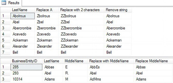
Figure 3-14. The partial results of using REPLACE
Nesting Functions
The previous section showed how to use one function at a time to manipulate strings. If the results of one expression must be used as a parameter of another function call, you can nest functions. For example, you can nest the LTRIM and RTRIM functions to remove the spaces from the beginning and ending of a string like this: LTRIM(RTRIM(' test ')). Keep in mind when writing nested functions you work from the inside out. The inner-most function is executed first and the outer functions execute against the results. Let’s look at some examples. Type in and execute the example shown in Listing 3-15 to display the domains in a list of e-mail addresses and the file name from a list of file paths.
Listing 3-15. Nesting Functions
USE AdventureWorks2012;

GO


--1

SELECT EmailAddress,

    SUBSTRING(EmailAddress,CHARINDEX('@',EmailAddress) + 1,50) AS DOMAIN

FROM Production.ProductReview;


--2

SELECT EmailAddress,

RIGHT(EmailAddress, CHARINDEX('@', REVERSE(EmailAddress))-1) AS DOMAIN

FROM Production.ProductReview;
Figure 3-15 shows the results. Query 1 first uses the CHARINDEX function to find the location of the at symbol (@). The results of that expression are used as a parameter to the outer SUBSTRING function. To display the characters after the @ symbol, add 1 to the position of the @ symbol.
Query 2 produces the same results but uses different commands. The query performs a SELECT command from the Production.ProductReview table. After the SELECT the inner REVERSE function reverses the string value. Then the outer CHARINDEX finds the location of the @ symbol and subtracts one character to remove it from the results. By using that result as the second parameter of the RIGHT function, the query returns the domain name. When writing a query like this, take it a step at a time and work from the inside out. You may have to experiment a bit to get it right.

Figure 3-15. The results of using nested functions
This section covered a sample of the many functions available to manipulate strings in T-SQL. Complete Exercise 3-3 to practice using these functions.
Using Date Functions
Just as T-SQL features a rich set of functions for working with string data, it also boasts an impressive list of functions for working with date and time data types. In this section, you’ll take a look at some of the most commonly used functions for date and time data.
GETDATE and SYSDATETIME
Use GETDATE or SYSDATETIME to return the current date and time of the server. The difference is that SYSDATETIME returns seven decimal places after the second, while GETDATE returns only three places. You may see zeros filling in some of the right digits if your SQL Server is installed on Vista-64 instead of another operating system.
GETDATE and SYSDATETIME are nondeterministic functions. This means that they return different values each time they are called. Most of the functions in this chapter are deterministic, which means that a function always returns the same value when called with the same parameters and database settings. For example, the code CHARINDEX('B','abcd') will always return 2 if the collation of the database is case insensitive. In a case-sensitive database, the expression will return 0.
Run this code several times to see how these functions work:
SELECT GETDATE(), SYSDATETIME();DATEADD
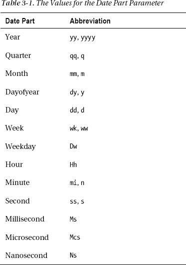
Use DATEADD to add a number of time units to a date. The function requires three parameters: the date part, the number, and a date. T-SQL doesn’t have a DATESUBTRACT function, but you can use a negative number to accomplish the same thing. You might use DATEADD to calculate an expiration date or a date that a payment is due, for example. Table 3-1 from Books Online lists the possible values for the date part parameter in the DATADD function and other date functions. Here is the syntax for DATEADD:
DATEADD(<date part>,<number>,<date>)
Type in and execute the code in Listing 3-16 to learn how to use the DATEADD function.
Listing 3-16. Using the DATEADD Function
Use AdventureWorks2012

GO

--1

SELECT OrderDate, DATEADD(year,1,OrderDate) AS OneMoreYear,

    DATEADD(month,1,OrderDate) AS OneMoreMonth,

    DATEADD(day,-1,OrderDate) AS OneLessDay

FROM Sales.SalesOrderHeader

WHERE SalesOrderID in (43659,43714,60621);

--2

SELECT DATEADD(month,1,'1/29/2009') AS FebDate;
Figure 3-16 shows the results of Listing 3-16. In query 1, the DATEADD function adds exactly the time unit specified in each expression to the OrderDate column from the Sales.SalesOrderHeader table. Notice in the results of query 2 that since there is no 29th day of February 2009, adding one month to January 29, 2009, returns February 28, the last possible day in February that year.
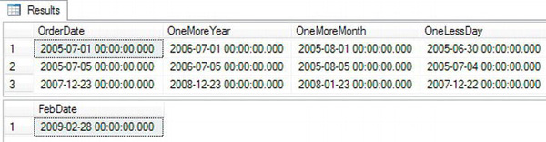
Figure 3-16. The results of using the DATEADD function
DATEDIFF
The DATEDIFF function allows you to find the difference between two dates. The function requires three parameters: the date part and the two dates. The DATEDIFF function might be used to calculate how many days have passed since unshipped orders were taken, for example. Here is the syntax:
DATEDIFF(<datepart>,<early date>,<later date>)
See Table 3-1 for the list of possible date parts. Listing 3-17 demonstrates how to use DATEDIFF. Be sure to type in and execute the code.
Use AdventureWorks2012;

GO


--1

SELECT OrderDate, GETDATE() CurrentDateTime,

    DATEDIFF(year,OrderDate,GETDATE()) AS YearDiff,

    DATEDIFF(month,OrderDate,GETDATE()) AS MonthDiff,

    DATEDIFF(day,OrderDate,GETDATE()) AS DayDiff

FROM Sales.SalesOrderHeader

WHERE SalesOrderID in (43659,43714,60621);


--2

SELECT DATEDIFF(year,'12/31/2008','1/1/2009') AS YearDiff,

    DATEDIFF(month,'12/31/2008','1/1/2009') AS MonthDiff,

    DATEDIFF(day,'12/31/2008','1/1/2009') AS DayDiff;
Figure 3-17 shows the results. Your results from query 1 will be different from mine since the query uses GETDATE(), a nondeterministic function, instead of hard-coded dates or dates from a table. Even though query 2 compares the difference between two dates that are just one day apart, the differences in years and months are both 1. The DATEDIFF rounds up the result to the nearest integer and doesn’t display decimal results.
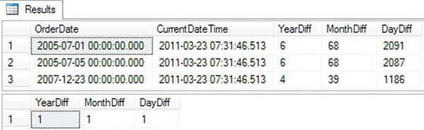
Figure 3-17. The results of using DATEDIFF
DATENAME and DATEPART
The DATENAME and DATEPART functions return the part of the date specified. Developers use the DATENAME and DATEPART functions to display just the year or month on reports, for example. DATEPART always returns a numeric value. DATENAME returns the actual name when the date part is the month or the day of the week. Again, you can find the possible date parts in Table 3-1. The syntax for the two functions is similar.
DATENAME(<datepart>,<date>)

DATEPART(<datepart>,<date>)
Type in and execute the code in Listing 3-18 to learn how to use DATENAME.
Listing 3-18. Using DATENAME and DATEPART
Use AdventureWorks2012

GO

--1

SELECT OrderDate, DATEPART(year,OrderDate) AS OrderYear,

    DATEPART(month,OrderDate) AS OrderMonth,

    DATEPART(day,OrderDate) AS OrderDay,

    DATEPART(weekday,OrderDate) AS OrderWeekDay

FROM Sales.SalesOrderHeader

WHERE SalesOrderID in (43659,43714,60621);


--2

SELECT OrderDate, DATENAME(year,OrderDate) AS OrderYear,

    DATENAME(month,OrderDate) AS OrderMonth,

    DATENAME(day,OrderDate) AS OrderDay,

    DATENAME(weekday,OrderDate) AS OrderWeekDay

FROM Sales.SalesOrderHeader

WHERE SalesOrderID in (43659,43714,60621);
Figure 3-18 displays the results. You will see that the results are the same except for spelling out the month and weekday in query 2. One other thing to keep in mind is that the value returned from DATEPART is always an integer, while the value returned from DATENAME is always a string, even when the expression returns a number.

Figure 3-18. Results of using DATENAME and DATEPART
DAY, MONTH, and YEAR
The DAY, MONTH, and YEAR functions work just like DATEPART. These functions are just alternate ways to get the day, month, or year from a date. Here is the syntax:
DAY(<date>)

MONTH(<date>)

YEAR(<date>)
Type in and execute the code in Listing 3-19 to see that this is just another way to get the same results as using the DATEPART function.
Listing 3-19. Using the DAY, MONTH, and YEAR Functions
Use AdventureWorks2012

GO


SELECT OrderDate, YEAR(OrderDate) AS OrderYear,

    MONTH(OrderDate) AS OrderMonth,

    DAY(OrderDate) AS OrderDay

FROM Sales.SalesOrderHeader

WHERE SalesOrderID in (43659,43714,60621);
Figure 3-19 displays the results of the code from Listing 3-19. If you take a look at the results of query 1 from Listing 3-18 that used the DATEPART function, you will see that they are the same.

Figure 3-19. The result of using YEAR, MONTH, and DAY
CONVERT
You learned about CONVERT earlier in the chapter when I talked about concatenating strings. To append a number or a date to a string, the number or date must first be cast to a string. The CONVERT function has an optional parameter called style that can be used to format a date.
I have frequently seen code that used the DATEPART function to break a date into its parts and then cast the parts into strings and concatenate them back together to format the date. It is so much easier just to use CONVERT to accomplish the same thing! Here is the syntax:
CONVERT(<data type, usually varchar>,<date>,<style>)
Type in and execute the code in Listing 3-20 to compare both methods of formatting dates. Take a look at the SQL Server Books Online article “CAST and CONVERT” for a list of all the possible formats.
Listing 3-20. Using CONVERT to Format a Date/Time Value
--1 The hard way!

SELECT CAST(DATEPART(YYYY,GETDATE()) AS VARCHAR) + '/' +

    CAST(DATEPART(MM,GETDATE()) AS VARCHAR) +

    '/' +  CAST(DATEPART(DD,GETDATE()) AS VARCHAR) AS DateCast;

--2 The easy way!

SELECT CONVERT(VARCHAR,GETDATE(),111) AS DateConvert;

--3

USE AdventureWorks2012

GO
SELECT CONVERT(VARCHAR,OrderDate,1) AS "1",

    CONVERT(VARCHAR,OrderDate,101) AS "101",

    CONVERT(VARCHAR,OrderDate,2) AS "2",

    CONVERT(VARCHAR,OrderDate,102) AS "102"

FROM Sales.SalesOrderHeader

WHERE SalesOrderID in (43659,43714,60621);
Figure 3-20 shows the results of Listing 3-20. Notice in query 1 that you not only had to use DATEPART three times, but you also had to cast each result to a VARCHAR in order to concatenate the pieces back together. Query 2 shows the easy way to accomplish the same thing. This method is often used to remove the time from a DATETIME data type. Query 3 demonstrates four different formats. Notice that the three-digit formats always produce four-digit years.

Figure 3-20. The results of formatting dates
FORMAT
SQL Server 2012 introduces the FORMAT function. The primary purpose is to simplify the conversion of date/time values as string values. Another purpose of the format function is to convert date/time values to their cultural equivalencies. Here is the syntax:
FORMAT ( value, format [, culture ] )
The FORMAT function greatly simplifies how date/time values are converted, and it should be used for date/time values instead of the CAST or CONVERT functions. Listing 3-21 shows some examples.
Listing 3-21. FORMAT Function Examples
DECLARE @d DATETIME = GETDATE();


SELECT FORMAT( @d, 'dd', 'en-US' ) AS Result;

SELECT FORMAT( @d, 'd/M/y', 'en-US' ) AS Result;

SELECT FORMAT( @d, 'dd/MM/yyyy', 'en-US' ) AS Result;
Figure 3-21 shows the results. Keep in mind the letters for each part of the date are case sensitive. For example if you switch mm for MM you will get back minutes instead of months.
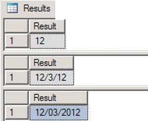
Figure 3-21. FORMAT Function Results
SQL 2012 also introduces a simple method to derive a date, time, or date and time from a list of values. The primary function is called DATEFROMPARTS but there is also a version of the function for time, and date and time. Listing 3-22 shows some examples.
Listing 3-22. DATEFROMPARTS Examples
SELECT DATEFROMPARTS(2012, 3, 10) AS RESULT;

SELECT TIMEFROMPARTS(12, 10, 32, 0, 0) AS RESULT;

SELECT DATETIME2FROMPARTS (2012, 3, 10, 12, 10, 32, 0, 0) AS RESULT;
Figure 3-22 shows the results from each function. The first function returns only the date. The TIMEFROMPARTS function returns a time. Finally, the DATETIME2FROMPARTS returns both a date and a time. If a value is out of the range of either a date or time, for example you put 13 for the month value, the function will throw an error.
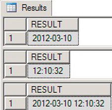
Figure 3-22. Results from DATEFROMTIME functions
This section covered a sample of the functions available for manipulating dates. Practice what you have learned by completing Exercise 3-4.
Using Mathematical Functions
You can use several mathematical functions on numeric values. These include trigonometric functions such as SIN and TAN and logarithmic functions that are not used frequently in business applications. This section discusses some of the more commonly used mathematical functions.
ABS
The ABS function returns the absolute value of the number—the difference between the number and zero. Type in and execute this code to see how to use ABS:
SELECT ABS(2) AS "2", ABS(-2) AS "-2"
POWER
The POWER function returns the power of one number to another number. The syntax is simple.
POWER(<number>,<power>)
There may not be many uses for POWER in business applications, but you may use it in scientific or academic applications. Type in and execute the code in Listing 3-23.
Listing 3-23. Using POWER
SELECT POWER(10,1) AS "Ten to the First",

    POWER(10,2) AS "Ten to the Second",

    POWER(10,3) AS "Ten to the Third";
Figure 3-23 displays the results. The POWER function returns a FLOAT value. Caution must be taken, however, with this function. The results will increase in size very quickly and can cause an overflow error. Try finding the value of 10 to the 10th power to see what can happen.

Figure 3-23. The results of using POWER
SQUARE and SQRT
The SQUARE function returns the square of a number, or the number multiplied to itself. The SQRT function returns the opposite, the square root of a number. Type in and execute the code in Listing 3-24 to see how to use these functions.
Listing 3-24. Using the SQUARE and SQRT Functions
SELECT SQUARE(10) AS "Square of 10",

    SQRT(10) AS "Square Root of 10",

    SQRT(SQUARE(10)) AS "The Square Root of the Square of 10";
Figure 3-24 shows the results. Notice that the third expression in the query is a nested function that squares 10 and then takes the square root of that result.
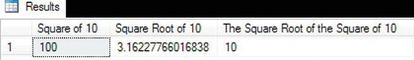
Figure 3-24. The results of using SQUARE and SQRT
ROUND
The ROUND function allows you to round a number to a given precision. The ROUND function is used frequently to display only the number of decimal places required in the report or application. The ROUND function requires two parameters, the number and the length, which can be either positive or negative. It also has an optional third parameter that causes the function to just truncate instead of rounding if a nonzero value is supplied. Here is the syntax:
ROUND(<number>,<length>[,<function>])
Type in and execute the code in Listing 3-25 to learn how to use ROUND.
Listing 3-25. Using ROUND
SELECT ROUND(1234.1294,2) AS "2 places on the right",

    ROUND(1234.1294,-2) AS "2 places on the left",

    ROUND(1234.1294,2,1) AS "Truncate 2",

    ROUND(1234.1294,-2,1) AS "Truncate -2";
You can view the results in Figure 3-25. When the expression contains a negative number as the second parameter, the function rounds on the left side of the decimal point. Notice the difference when 1 is used as the third parameter, causing the function to truncate instead of rounding. When rounding 1234.1294, the expression returns 1234.1300. When truncating 1234.1294, the expression returns 1234.1200. It doesn’t round the value; it just changes the specified digits to zero.

Figure 3-25. The results of using ROUND
RAND
RAND returns a float value between 0 and 1. RAND can be used to generate a random value. This might be used to generate data for testing an application, for example. The RAND function takes one optional integer parameter, @seed. When the RAND expression contains the seed value, the function returns the same value each time. If the expression doesn’t contain a seed value, SQL Server randomly assigns a seed, effectively providing a random number. Type in and execute the code in Listing 3-26 to generate a random numbers.
SELECT CAST(RAND() * 100 AS INT) + 1 AS "1 to 100",

    CAST(RAND()* 1000 AS INT) + 900 AS "900 to 1900",

    CAST(RAND() * 5 AS INT)+ 1 AS "1 to 5";
Since the function returns a float value, multiply by the size of the range, and add the lower limit (see Figure 3-26). The first expression returns random numbers between 1 and 100. The second expression returns random numbers between 900 and 1,900. The third expression returns random values between 1 and 5.

Figure 3-26. The results of generating random numbers with RAND
If you supply a seed value to one of the calls to RAND within a batch of statements, that seed affects the other calls. The value is not the same, but the values are predictable. Run this statement several times to see what happens when a seed value is used:
SELECT RAND(3),RAND(),RAND().
Just like strings and dates, you will find several functions that manipulate numbers. Practice using these functions by completing Exercise 3-5.
System Functions
T-SQL features many other built-in functions. Some are specific for administering SQL Server, while others are very useful in regular end user applications, returning information such as the database and current usernames. Be sure to review the “Functions” topic in Books Online often to discover functions that will make your life easier.
The CASE Function
Use the CASE function to evaluate a list of expressions and return the first one that evaluates to true. For example, a report may need to display the season of the year based on one of the date columns in the table. CASE is similar to Select Case or Switch used in other programming languages, but it is used inside the statement.
There are two ways to write a CASE expression: simple or searched. The following sections will explain the differences and how to use them.
Simple CASE
To write the simple CASE statement, come up with an expression that you want to evaluate, often a column name, and a list of possible values. Here is the syntax:
CASE <test expression>

    WHEN <comparison expression1> THEN <return value1>

    WHEN <comparison expression2> THEN <return value2>

    [ELSE <value3>] END
Type in and execute the code in Listing 3-27 to learn how to use the simple version of CASE.
Listing 3-27. Using Simple CASE
USE AdventureWorks2012;

GO

SELECT Title,

    CASE Title

    WHEN 'Mr.' THEN 'Male'

    WHEN 'Ms.' THEN 'Female'

    WHEN 'Mrs.' THEN 'Female'

    WHEN 'Miss' THEN 'Female'

    ELSE 'Unknown' END AS Gender

FROM Person.Person

WHERE BusinessEntityID IN (1,5,6,357,358,11621,423);
Figure 3-27 shows the results. Even though the CASE statement took up a lot of room in the query, it is producing only one column in the results. For each row returned, the expression evaluates the Title column to see whether it matches any of the possibilities listed and returns the appropriate value. If the value from Title doesn’t match or is NULL, then whatever is in the ELSE part of the expression is returned. If no ELSE exists, the expression returns NULL.
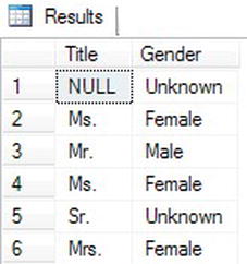
Figure 3-27. The results of using simple CASE
Searched CASE
Developers often used the searched CASE syntax when the expression is too complicated for the simple CASE syntax. For example, you might want to compare the value from a column to several IN lists or use greater-than or less-than operators. The CASE statement returns the first expression that returns true. This is the syntax for the searched CASE:
CASE WHEN <test expression1> THEN <value1>

WHEN <test expression2> THEN <value2>

[ELSE <value3>] END
Type in and execute the code in Listing 3-28 to learn how to use this more flexible method of using CASE.
Listing 3-28. Using Searched CASE
SELECT Title,

    CASE WHEN Title IN ('Ms.','Mrs.','Miss') THEN 'Female'

    WHEN Title = 'Mr.' THEN 'Male'

    ELSE 'Unknown' END AS Gender

FROM Person.Person

WHERE BusinessEntityID IN (1,5,6,357,358,11621,423);
This query returns the same results (see Figure 3-28) as the one in Listing 3-27. The CASE function evaluates each WHEN expression independently until finding the first one that returns true. It then returns the appropriate value. If none of the expressions returns true, the function returns the value from the ELSE part or NULL if no ELSE is available.
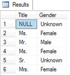
Figure 3-28. The results of using searched CASE
One very important note about using CASE is that the return values must be of compatible data types. For example, you can’t have one part of the expression returning an integer while another part returns a non-numeric string. Precedence rules apply as with other operations.
Listing a Column as the Return Value
It is also possible to list a column name instead of hard-coded values in the THEN part of the CASE function. This means that you can display one column for some of the rows and another column for other rows. Type in and execute the code in Listing 3-29 to see how this works.
Listing 3-29. Returning a Column Name in CASE
USE AdventureWorks2012;

GO


SELECT VacationHours,SickLeaveHours,

    CASE WHEN VacationHours > SickLeaveHours THEN VacationHours

    ELSE SickLeaveHours END AS 'More Hours'

FROM HumanResources.Employee;
In this example (see Figure 3-29), if there are more VacationHours than SickLeaveHours, the query displays the VacationHours column from the HumanResources.Empoyee table in the More Hours column. Otherwise, the query returns the SickLeaveHours.
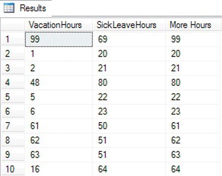
Figure 3-29. The results of returning a column from CASE
IIF
SQL 2012 introduces one easier method of writing a simple CASE statement. In SQL 2012 you can now use an IIF statement to return a result based on whether or not a Boolean expression is true or false. To create an IFF statement you need a Boolean expression and the values to return based on the results. Here is the basic syntax for the IIF statement.
IIF ( boolean_expression, true_value, false_value )
Execute the code in Listing 3-30. The first IIF statement is a simple execution while the second IFF shows how you can introduce varibles into the statement.
Listing 3-30. IIF Statement
--IIF Statement without variables


SELECT IIF (50 > 20, 'TRUE', 'FALSE') AS RESULT;


--IIF Statement with variables


DECLARE @a INT = 50

DECLARE @b INT = 25

SELECT IIF (@a > @b, 'TRUE', 'FALSE') AS RESULT;
Figure 3-30 shows the results. Keep in mind that all rules which apply to CASE statements also apply to IIF statements.

Figure 3-30. Results of IFF Statements
COALESCE
You learned about COALESCE earlier in the chapter in the “Concatenating Strings and NULL” section. You can use COALESCE with other data types as well and with any number of arguments to return the first non-NULL value. You can use the COALESCE function in place of ISNULL. If a list of values must be evaluated instead of one value, you must use COALESCE instead of ISNULL. COALESCE may be used when concatenating strings or any time that a replacement for NULL must be found. Type in and execute the code in Listing 3-31 to learn more about COALESCE.
Listing 3-31. Using COALESCE
USE AdventureWorks2012;

GO


SELECT ProductID,Size, Color,

    COALESCE(Size, Color,'No color or size') AS 'Description'

FROM Production.Product

where ProductID in (1,2,317,320,680,706);
Figure 3-31 displays the results. The COALESCE expression first checks the Size value and then the Color value to find the first non-NULL value. If both values are NULL, then the string No color or size is returned.
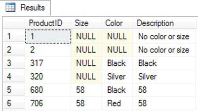
Figure 3-31. The results of using COALESCE
Admin Functions
T-SQL contains many administrative functions that are useful for developers. SQL Server also has many functions that help database administrators manage SQL Server; these functions are beyond the scope of this book. Listing 3-32 shows a few examples of functions that return information about the current connection such as the database name and application.
Listing 3-32. A Few System Functions
SELECT DB_NAME() AS "Database Name",

    HOST_NAME() AS "Host Name",

    CURRENT_USER AS "Current User",

    USER_NAME() AS "User Name",

    APP_NAME() AS "App Name";
Take a look at Figure 3-32 for my results; your results will probably be different. When I ran the query, I was connected to the AdventureWorks2012 database on a computer named WIN-5RUBLZ7G773 as the dbo (database owner) user while using Management Studio.

Figure 3-32. The results of using system functions
In addition to the functions used to manipulate strings, dates, and numbers, you will find many system functions. Some of these work on different types of data, such as CASE, while others provide information about the current connection. Administrators can manage SQL Server using dozens of system functions not covered in this book. Complete Exercise 3-6 to practice using the system functions covered in this section.
Using Functions in the WHERE and ORDER BY Clauses
So far you have seen functions used in the SELECT list. You may also use functions in the WHERE and ORDER BY clauses. Take a look at Listing 3-33 for several examples.
Listing 3-33. Using Functions in WHERE and ORDER BY
USE AdventureWorks2012;

GO


--1

SELECT FirstName

FROM Person.Person

WHERE CHARINDEX('ke',FirstName) > 0;


--2

SELECT LastName,REVERSE(LastName)

FROM Person.Person

ORDER BY REVERSE(LastName);


--3

SELECT BirthDate

FROM HumanResources.Employee

ORDER BY YEAR(BirthDate);
Figure 3-33 shows the results of Listing 3-34. Even though it is very easy to use a function on a column in the WHERE clause, it is important to note that performance may suffer. If the database designer created an index on the searched column, the database engine must evaluate each row one at a time when a function is applied to a column.
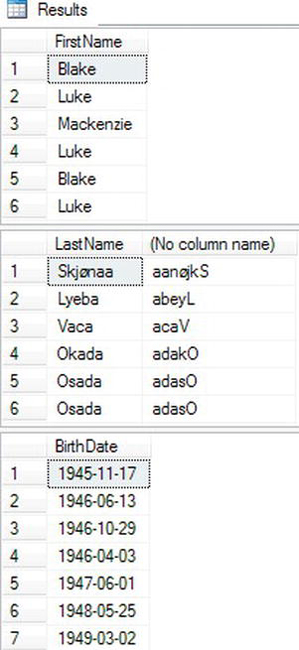
Figure 3-33. The results of using functions in the WHERE and ORDER BY clauses
Practice using functions in the WHERE and ORDER by clauses by completing Exercise 3-7.
The TOP Keyword
Use the TOP keyword to limit the number or percentage of rows returned from a query. TOP has been around for a long time, but beginning with the release of SQL Server 2005, Microsoft has added several enhancements. TOP originally could be used in SELECT statements only. You could not use TOP in a DELETE, UPDATE, or INSERT statement. The number or percentage specified had to be a hard-coded value. SQL Server 2012You can use TOP in data manipulation statements and use a variable to specify the number or percentage or rows. Here is the syntax:
SELECT TOP(<number>) [PERCENT] [WITH TIES] <col1>,<col2>

FROM <table1> [ORDER BY <col1>]


DELETE TOP(<number>) [PERCENT] [FROM] <table1>


UPDATE TOP(<number>) [PERCENT] <table1> SET <col1> = <value>


INSERT TOP(<number>) [PERCENT] [INTO] <table1> (<col1>,<col2>)

SELECT <col3>,<col4> FROM <table2>


INSERT [INTO] <table1> (<col1>,<col2>)

SELECT TOP(<numbers>) [PERCENT] <col3>,<col4>

FROM <table2>

ORDER BY <col1>
The ORDER BY clause is optional with the SELECT statement, but most of the time, you will use it to determine which rows the query returns. A scenario you may want to select random rows is if you need to select sample data in order to populate a test environment. Otherwise, it rarely makes sense to request the TOP N random rows. Usually one sorts by some criteria in order to get the TOP N rows in that sequence.
The ORDER BY clause is not valid with DELETE and UPDATE. The WITH TIES option is valid only with the SELECT statement. It means that, if there are rows that have identical values in the ORDER BY clause, the results will include all the rows even though you now end up with more rows than you expect. Type in and execute the code in Listing 3-34 to learn how to use TOP.
Listing 3-34. Limiting Results with TOP
USE AdventureWorks2012;

GO


--1

IF OBJECT_ID('dbo.Sales') IS NOT NULL BEGIN

    DROP TABLE dbo.Sales;

END;


--2

CREATE TABLE dbo.Sales (CustomerID INT, OrderDate DATE,

    SalesOrderID INT NOT NULL PRIMARY KEY);

GO


--3

INSERT TOP(5) INTO dbo.Sales(CustomerID,OrderDate,SalesOrderID)

SELECT CustomerID, OrderDate, SalesOrderID

FROM Sales.SalesOrderHeader;


--4

SELECT CustomerID, OrderDate, SalesOrderID

FROM dbo.Sales

ORDER BY SalesOrderID;


--5

DELETE TOP(2) dbo.Sales


--6

UPDATE TOP(2) dbo.Sales SET CustomerID = CustomerID + 10000;


--7

SELECT CustomerID, OrderDate, SalesOrderID

FROM dbo.Sales

ORDER BY SalesOrderID;


--8

DECLARE @Rows INT = 2;

SELECT TOP(@Rows) CustomerID, OrderDate, SalesOrderID

FROM dbo.Sales

ORDER BY SalesOrderID;
Figure 3-34 shows the results. Code section 1 drops the dbo.Sales table if it exists. Statement 2 creates the table. Statement 3 inserts five rows into the dbo.Sales table. Using TOP in the INSERT part of the statement doesn’t allow you to use ORDER BY to determine which rows to insert. To control which rows get inserted, move TOP to the SELECT statement. Query 4 shows the inserted rows. Statement 5 deletes two of the rows. Statement 6 updates the CustomerID of two of the rows. Query 7 shows how the data looks after the delete and update. Code section 8 shows how to use a variable with TOP.

Figure 3-34. The results of using TOP
![]() Note Microsoft recommends using the
Note Microsoft recommends using the OFFSET and FETCH clauses instead of TOP as a paging solution and to limit the amount of data sent to a client. OFFSET and FETCH also allow more options, including the use of variables.
Ranking Functions
Ranking functions introduced with SQL Server 2005 allow you to assign a number to each row returned from a query. For example, suppose you need to include a row number with each row for display on a web page. You could come up with a method to do this, such as inserting the query results into a temporary table that includes an IDENTITY column, but now you can create the numbers by using the ROW_NUMBER function. During your T-SQL programming career, you will probably find you can solve many query problems by including ROW_NUMBER. Recently I needed to insert several thousand rows into a table that included a unique ID. I was able to add the maximum ID value already in the table to the result of the ROW_NUMBER function to successfully insert the new rows. Along with ROW_NUMBER, this section covers RANK, DENSE_RANK, and NTILE.
Using ROW_NUMBER
The ROW_NUMBER function returns a sequential numeric value along with the results of a query. The ROW_NUMBER function contains the OVER clause, which the function uses to determine the numbering behavior. You must include the ORDER BY option, which determines the order in which the function applies the numbers. You have the option of starting the numbers over whenever the values of a specified column change, called partitioning, with the PARTITION BY clause. One limitation with using ROW_NUMBER is that you can’t include it in the WHERE clause. To filter the rows, include the query containing ROW_NUMBER in a CTE (you will learn about common table expressions in Chapter 10), and then filter on the ROW_NUMBER alias in the outer query. Here is the syntax:
SELECT <col1>,<col2>,

    ROW_NUMBER() OVER([PARTITION BY <col1>,<col2>]

        ORDER BY <col1>,<col2>) AS <RNalias>

FROM <table1>


WITH <cteName> AS (

    SELECT <col1>,<col2>,

        ROW_NUMBER() OVER([PARTITION BY <col1>,<col2>]

            ORDER BY <col1>,<col2>) AS <RNalias>

    FROM <table1>)

SELECT <col1>,<col2>,<RNalias>

FROM <table1>

WHERE <criteria including RNalias>
Type in and execute Listing 3-35 to learn how to use ROW_NUMBER.
Listing 3-35. Using ROW_NUMBER
USE AdventureWorks2012;

GO


--1

SELECT CustomerID, FirstName + ' ' + LastName AS Name,

    ROW_NUMBER() OVER (ORDER BY LastName, FirstName) AS Row

FROM Sales.Customer AS c INNER JOIN Person.Person AS p

ON c.PersonID = p.BusinessEntityID;


--2

WITH customers AS (

    SELECT CustomerID, FirstName + ' ' + LastName AS Name,

        ROW_NUMBER() OVER (ORDER BY LastName, FirstName) AS Row

    FROM Sales.Customer AS c INNER JOIN Person.Person AS p

    ON c.PersonID = p.BusinessEntityID

    )

SELECT CustomerID, Name, Row

FROM customers

WHERE Row > 50

ORDER BY Row;


--3

SELECT CustomerID, FirstName + ' ' + LastName AS Name, c.TerritoryID,

    ROW_NUMBER() OVER (PARTITION BY c.TerritoryID

        ORDER BY LastName, FirstName) AS Row

FROM Sales.Customer AS c INNER JOIN Person.Person AS p

ON c.PersonID = p.BusinessEntityID;
Figure 3-35 shows the partial results. Query 1 assigns the row numbers in order of LastName, FirstName to the query joining the Sales.Customer table to the Person.Person table. Each row in the results contains a unique row number.
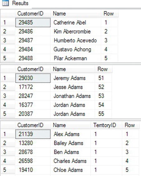
Figure 3-35. The partial results of using ROW_NUMBER
Query 2 demonstrates how you can include the row number in the WHERE clause by using a CTE. The CTE in query 2 contains the same code as query 1. Now the Row column is available to you to use in the WHERE clause just like any other column. By using this technique, you can apply the WHERE clause to the results of the ROW_NUMBER function, and only the rows with a row number exceeding 50 appear in the results.
Query 3 uses the PARTITION BY option to start the row numbers over on each TerritoryID. The results shown in Figure 3-30 show the end of TerritoryID 1 and the beginning of TerritoryID 2.
Using RANK and DENSE_RANK
RANK and DENSE_RANK are very similar to ROW_NUMBER. The difference is how the functions deal with ties in the ORDER BY values. RANK assigns the same number to the duplicate rows and skips numbers not used. DENSE_RANK doesn’t skip numbers. For example, if rows 2 and 3 are duplicates, RANK will supply the values 1, 3, 3, and 4, and DENSE_RANK will supply the values 1, 2, 2, and 3. Here is the syntax:
--1 RANK exampple

SELECT <col1>, RANK() OVER([PARTITION BY <col2>,<col3>] ORDER BY <col1>,<col2>)

FROM <table1>


--2 DENSE_RANK example

SELECT <col2>, DENSE_RANK() OVER([PARTITION BY <col2>,<col3>]

    ORDER BY <col1>,<col2>)

FROM <table1>
Type in and execute the code in Listing 3-36 to learn how to use RANK and DENSE_RANK.
Listing 3-36. Using RANK and DENSE_RANK
USE AdventureWorks2012;

GO


SELECT CustomerID,COUNT(*) AS CountOfSales,

    RANK() OVER(ORDER BY COUNT(*) DESC) AS Ranking,

    ROW_NUMBER() OVER(ORDER BY COUNT(*) DESC) AS Row,

    DENSE_RANK() OVER(ORDER BY COUNT(*) DESC) AS DenseRanking

FROM Sales.SalesOrderHeader

GROUP BY CustomerID

ORDER BY COUNT(*) DESC;
Figure 3-36 shows the partial results. The query compares ROW_NUMBER to RANK and DENSE_RANK. In each expression, the count of the sales for each customer determines the order of the numbers.
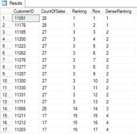
Figure 3-36. The partial results of using RANK and DENSE_RANK
Using NTILE
While the other ranking functions supply a row number or rank to each row, the NTILE function assigns buckets to groups of rows. For example, suppose the AdventureWorks company wants to divide up bonus money for the sales staff. You can use the NTILE function to divide up the money based on the sales by each employee. Here is the syntax:
SELECT <col1>, NTILE(<buckets>) OVER([PARTITION BY <col1>,<col1>]

    ORDER BY <col1>,<col2>) AS <alias>

FROM <table1>
Type in and execute Listing 3-37 to learn how to use NTILE.
Listing 3-37. Using NTILE
USE AdventureWorks2012;

GO


SELECT SalesPersonID,SUM(TotalDue) AS TotalSales,

    NTILE(10) OVER(ORDER BY SUM(TotalDue)) * 10000/COUNT(*) OVER() AS Bonus

FROM Sales.SalesOrderHeader

WHERE SalesPersonID IS NOT NULL

    AND OrderDate BETWEEN '1/1/2005' AND '12/31/2005'

GROUP BY SalesPersonID

ORDER BY TotalSales;
Figure 3-37 shows the results. The query returns the sum of the total sales grouped by the SalesPersonID for 2005. The NTILE function divides the rows into 10 groups, or buckets, based on the sales for each salesperson. The query multiplies the value returned by the NTILE expression by 10,000 divided by the number of rows to determine the bonus amount. The query uses the COUNT(*) OVER() expression to determine the number of rows in the results. See “The OVER Clause” in Chapter 5 to review how this works.
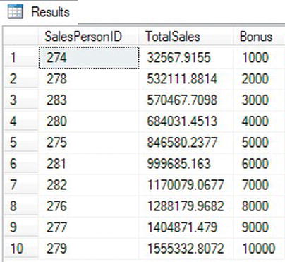
Figure 3-37. The results of using NTILE
The salespeople with the lowest sales get the smallest bonuses. The salespeople with the highest sales get the biggest bonuses. Notice that the smaller values have two rows in each bucket, but the last three buckets each have one row. The query must produce ten buckets, but there are not enough rows to divide the buckets up evenly.
Thinking About Performance
In Chapter 2 you learned how to use execution plans to compare two or more queries and determine which query uses the least resources or, in other words, performs the best. In this chapter, you will see how using functions can affect performance. Review the “Thinking About Performance” section in Chapter 2 if you need to take another look at how to use execution plans or to brush up on how SQL Server uses indexes.
Using Functions in the WHERE Clause
In the section “Using Functions in the WHERE and ORDER BY Clauses,” you learned that functions can be used in the WHERE clause to filter out unneeded rows. Although I am not saying that you should never include a function in the WHERE clause, you need to realize that including a function that operates on a column may cause a decrease in performance.
The Sales.SalesOrderHeader table does not contain an index on the OrderDate column. Run the following code to create an index on the column. Don’t worry about trying to understand the code at this point.
USE AdventureWorks2012

GO

--Add an index

IF  EXISTS (SELECT * FROM sys.indexes WHERE object_id =

    OBJECT_ID(N'[Sales].[SalesOrderHeader]')

    AND name = N'DEMO_SalesOrderHeader_OrderDate')

DROP INDEX [DEMO_SalesOrderHeader_OrderDate]

    ON [Sales].[SalesOrderHeader] WITH ( ONLINE = OFF );

GO

CREATE NONCLUSTERED INDEX [DEMO_SalesOrderHeader_OrderDate]

    ON [Sales].[SalesOrderHeader]

([OrderDate] ASC);
Toggle on the Include Actual Execution Plan setting before typing and executing the code in Listing 3-38.
Listing 3-38. Compare the Performance When Using a Function in the WHERE Clause
USE AdventureWorks2012;

GO


--1

SELECT SalesOrderID, OrderDate

FROM Sales.SalesOrderHeader

WHERE OrderDate >= '2005-01-01 00:00:00'

    AND OrderDate <= '2006-01-01 00:00:00';
--2

SELECT SalesOrderID, OrderDate

FROM Sales.SalesOrderHeader

WHERE YEAR(OrderDate) = 2005;
Query 1 finds all the orders placed in 2005 without using a function. Query 2 uses the YEAR function to return the same results. Take a look at the execution plans (Figure 3-38) to see that query 1 performs much better with a query cost of 7 percent. When executing query 2, the database engine performs a scan of the entire index to see whether the result of the function applied to each value meets the criteria. The database engine performs a seek of the index in query 1 because it just has to compare the actual values, not the results of the function for each value.

Figure 3-38. The execution plans showing that using a function in the WHERE clause can affect performance
Remove the index you created for this demonstration by running this code:
IF  EXISTS (SELECT * FROM sys.indexes WHERE object_id =

    OBJECT_ID(N'[Sales].[SalesOrderHeader]')

    AND name = N'DEMO_SalesOrderHeader_OrderDate')

DROP INDEX [DEMO_SalesOrderHeader_OrderDate]

    ON [Sales].[SalesOrderHeader] WITH ( ONLINE = OFF );
Run Listing 3-38 again now that the index is gone. Figure 3-39 shows that with no index on the OrderDate column, the performance is almost identical. Now the database engine must perform a scan of the table (in this case, the clustered index) to find the correct rows in both of the queries. Notice that the execution plan suggests an index to help the performance of query 1. It doesn’t suggest an index for query 2 since an index won’t help.
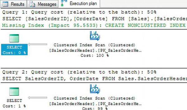
Figure 3-39. The execution plans after removing the index
You can see from these examples that writing queries is more than just getting the correct results; performance is important, too. Complete Exercise 3-8 to learn how using a function compares to a wildcard search.
Summary
Using expressions in T-SQL with the built-in functions and operators can be very convenient. There is a rich collection of functions for string and date manipulation as well as mathematical and system functions and more. It’s possible to use expressions and functions in the SELECT, WHERE, and ORDER BY clauses. You must use caution when using functions in the WHERE clause; it is possible to decrease performance.