C H A P T E R 5
Grouping and Summarizing Data
So far, you have learned to write simple queries that include filtering and ordering. You can also work with expressions built with operators and functions. The previous chapter taught you how to write queries with multiple tables so that the data makes sense in applications and reports. Now it’s time to learn about a special type of query, aggregate queries, used to group and summarize data. You may find that writing aggregate queries is more challenging than the other queries you have learned so far, but by taking a step-by-step approach, you will see that they are not difficult to write at all. Be sure to take the time to understand the examples and complete all the exercises before moving on to the next section.
Aggregate Functions
You use aggregate functions to summarize data in queries. The functions that you worked with in Chapter 3 operate on one value at a time. These functions operate on sets of values from multiple rows all at once. For example, you may need to supply information about how many orders were placed and the total amount ordered for a report. Here are the most commonly used aggregate functions:
COUNT: Counts the number of rows or the number of non-NULLvalues in a column.SUM: Adds up the values in numeric or money data.AVG: Calculates the average in numeric or money data.MIN: Finds the lowest value in the set of values. This can be used on string data as well as numeric, money, or date data.MAX: Finds the highest value in the set of values. This can be used on string data as well as numeric, money, or date data.
Keep the following in mind when working with these aggregate functions:
- The functions
AVGandSUMwill operate only on numeric and money data columns.- The functions
MIN,MAX, andCOUNTwill work on numeric, money, string, and temporal data columns.- The aggregate functions will not operate on
TEXT,NTEXT, andIMAGEcolumns. These data types are deprecated, meaning that they may not be supported in future versions of SQL Server.- The aggregate functions ignore
NULLvalues.COUNTcan be used with an asterisk (*) to give the count of the rows even if all the columns areNULL.- Once an aggregate function is used in a query, the query becomes an aggregate query.
Here is the syntax for the simplest type of aggregate query where the aggregate function is used in the SELECT list:
SELECT <aggregate function>(<col1>)

FROM <table>
Listing 5-1 shows an example of using aggregate functions. Type in and execute the code to learn how these functions are used over the entire result set.
Listing 5-1. Using Aggregate Functions
USE AdventureWorks2012;

GO


--1

SELECT COUNT(*) AS CountOfRows,

    MAX(TotalDue) AS MaxTotal,

    MIN(TotalDue) AS MinTotal,

    SUM(TotalDue) AS SumOfTotal,

    AVG(TotalDue) AS AvgTotal

FROM Sales.SalesOrderHeader;


--2

SELECT MIN(Name) AS MinName,

    MAX(Name) AS MaxName,

    MIN(SellStartDate) AS MinSellStartDate

FROM Production.Product;
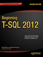
Take a look at the results in Figure 5-1. The aggregate functions operate on all the rows in the Sales.SalesOrderHeader table in query 1 and return just one row of results. The first expression, CountOfRows, uses an asterisk (*) to count all the rows in the table. The other expressions perform calculations on the TotalDue column. Query 2 demonstrates using the MIN and MAX functions on string and date columns. In these examples, the SELECT clause lists only aggregate expressions. You will learn how to add columns that are not part of aggregate expressions in the next section.
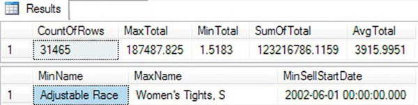
Figure 5-1. The results of using aggregate functions
Now that you know how to use aggregate functions to summarize a result set, practice what you have learned by completing Exercise 5-1.
The GROUP BY Clause
The previous example query and exercise questions listed only aggregate expressions in the SELECT list. The aggregate functions operated on the entire result set in each query. By adding more nonaggregated columns to the SELECT list, you add grouping levels to the query, which requires the use of the GROUP BY clause. The aggregate functions then operate on the grouping levels instead of on the entire set of results. This section covers grouping on columns and grouping on expressions.
Grouping on Columns
You can use the GROUP BY clause to group data so that the aggregate functions apply to groups of values instead of the entire result set. For example, you may want to calculate the count and sum of the orders placed, grouped by order date or grouped by customer. Here is the syntax for the GROUP BY clause:
SELECT <aggregate function>(<col1>), <col2>

FROM <table>

GROUP BY <col2>
One big difference you will notice once the query contains a GROUP BY clause is that additional nonaggregated columns may be included in the SELECT list. Once nonaggregated columns are in the SELECT list, you must add the GROUP BY clause and include all the nonaggregated columns. Run this code example, and view the error message:
USE AdventureWorks2012;

GO

SELECT CustomerID,SUM(TotalDue) AS TotalPerCustomer

FROM Sales.SalesOrderHeader;
Figure 5-2 shows the error message. To get around this error, add the GROUP BY clause and include nonaggregated columns in that clause. Make sure that the SELECT list includes only those columns that you really need in the results, because the SELECT list directly affects which columns will be required in the GROUP BY clause.

Figure 5-2. The error message that results when the required GROUP BY clause is missing
Type in and execute the code in Listing 5-2, which demonstrates how to use GROUP BY.
Listing 5-2. Using the GROUP BY Clause
USE AdventureWorks2012;

GO


--1

SELECT CustomerID,SUM(TotalDue) AS TotalPerCustomer

FROM Sales.SalesOrderHeader

GROUP BY CustomerID;


--2

SELECT TerritoryID,AVG(TotalDue) AS AveragePerTerritory

FROM Sales.SalesOrderHeader

GROUP BY TerritoryID;
Take a look at the results in Figure 5-3. Query 1 displays every customer with orders along with the sum of the TotalDue for each customer. The results are grouped by the CustomerID, and the sum is applied over each group of rows. Query 2 returns the average of the TotalDue values grouped by the TerritoryID. In each case, the nonaggregated column in the SELECT list must appear in the GROUP BY clause.

Figure 5-3. The results of using the GROUP BY clause
Any columns listed that are not part of an aggregate expression must be used to group the results. Those columns must be included in the GROUP BY clause. If you don’t want to group on a column, don’t list it in the SELECT list. This is where developers struggle when writing aggregate queries, so I can’t stress it enough.
Grouping on Expressions
The previous examples demonstrated how to group on columns, but it is possible to also group on expressions. You must include the exact expression from the SELECT list in the GROUP BY clause. Listing 5-3 demonstrates how to avoid incorrect results caused by adding a column instead of the expression to the GROUP BY clause.
Listing 5-3. How to Group on an Expression
Use AdventureWorks2012;

GO


--1

SELECT COUNT(*) AS CountOfOrders, YEAR(OrderDate) AS OrderYear

FROM Sales.SalesOrderHeader

GROUP BY OrderDate;
--2

SELECT COUNT(*) AS CountOfOrders, YEAR(OrderDate) AS OrderYear

FROM Sales.SalesOrderHeader

GROUP BY YEAR(OrderDate);
You can find the results in Figure 5-4. Notice that query 1 will run, but instead of returning one row per year, the query returns multiple rows with unexpected values. Because the GROUP BY clause contains OrderDate, the grouping is on OrderDate. The CountOfOrders expression is the count by OrderDate, not OrderYear. The expression in the SELECT list just changes how the data displays; it doesn’t affect the calculations.
Query 2 fixes this problem by including the exact expression from the SELECT list in the GROUP BY clause. Query 2 returns only one row per year, and CountOfOrders is correctly calculated.
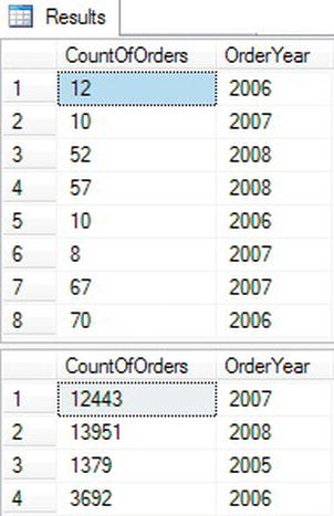
Figure 5-4. Using an expression in the GROUP BY clause
You use aggregate functions along with the GROUP BY clause to summarize data over groups of rows. Be sure to practice what you have learned by completing Exercise 5-2.
The ORDER BY Clause
You already know how to use the ORDER BY clause, but special rules exist for using the ORDER BY clause in aggregate queries. If a nonaggregate column appears in the ORDER BY clause, it must also appear in the GROUP BY clause, just like the SELECT list. Here is the syntax:
SELECT <aggregate function>(<col1>),<col2>

FROM <table1>

GROUP BY <col2>

ORDER BY <col2>
Type in the following code to see the error that results when a column included in the ORDER BY clause is missing from the GROUP BY clause:
USE AdventureWorks2012;

GO


SELECT CustomerID,SUM(TotalDue) AS TotalPerCustomer

FROM Sales.SalesOrderHeader

GROUP BY CustomerID

ORDER BY TerritoryID;
Figure 5-5 shows the error message that results from running the code. To avoid this error, make sure that you add only those columns to the ORDER BY clause that you intend to be grouping levels.

Figure 5-5. The error message resulting from including a column in the ORDER BY clause that is not a grouping level
Listing 5-4 demonstrates how to use the ORDER BY clause within an aggregate query. Be sure to type in and execute the code.
USE AdventureWorks2012;

GO


--1

SELECT CustomerID,SUM(TotalDue) AS TotalPerCustomer

FROM Sales.SalesOrderHeader

GROUP BY CustomerID

ORDER BY CustomerID;


--2

SELECT TerritoryID,AVG(TotalDue) AS AveragePerTerritory

FROM Sales.SalesOrderHeader

GROUP BY TerritoryID

ORDER BY TerritoryID;


--3

SELECT CustomerID,SUM(TotalDue) AS TotalPerCustomer

FROM Sales.SalesOrderHeader

GROUP BY CustomerID

ORDER BY SUM(TotalDue) DESC;
View the results of Listing 5-4 in Figure 5-6. As you can see, the ORDER BY clause follows the same rules as the SELECT list. Queries 1 and 2 return the results in the order of the nonaggregated column that is listed in the GROUP BY clause. Query 3 displays the results in the order of the sum of TotalDue in descending order.

The WHERE Clause
The WHERE clause in an aggregate query may contain anything allowed in the WHERE clause in any other query type. It may not, however, contain an aggregate expression. You use the WHERE clause to eliminate rows before the groupings and aggregates are applied. To filter after the groupings are applied, you will use the HAVING clause. You’ll learn about HAVING in the next section. Type in and execute the code in Listing 5-5, which demonstrates using the WHERE clause in an aggregate query.
Listing 5-5. Using the WHERE Clause
USE AdventureWorks2012;

GO

SELECT CustomerID,SUM(TotalDue) AS TotalPerCustomer

FROM Sales.SalesOrderHeader

WHERE TerritoryID in (5,6)

GROUP BY CustomerID;
The results in Figure 5-7 contain only those rows where the TerritoryID is either 5 or 6. The query eliminates the rows before the grouping is applied. Notice that TerritoryID doesn’t appear anywhere in the query except for the WHERE clause. The WHERE clause may contain any of the columns in the table as long as it doesn't contain an aggregate expression.

Figure 5-7. The results of using the WHERE clause in an aggregate query
The HAVING Clause
To eliminate rows based on an aggregate expression, use the HAVING clause. The HAVING clause may contain aggregate expressions that do or do not appear in the SELECT list. For example, you could write a query that returns the sum of the total due for customers who have placed at least ten orders. The count of the orders doesn’t have to appear in the SELECT list. Alternately, you could include only those customers who have spent at least $10,000 (sum of total due), which does appear in the list.
You can also include nonaggregate columns in the HAVING clause as long as the columns appear in the GROUP BY clause. In other words, you can eliminate some of the groups with the HAVING clause. Behind the scenes, however, the database engine may move that criteria to the WHERE clause because it is more efficient to eliminate those rows first. Criteria involving nonaggregate columns actually belongs in the WHERE clause, but the query will still work with the criteria appearing in the HAVING clause.
Most of the operators such as equal to (=), less than (<), and between that are used in the WHERE clause will work. Here is the syntax:
SELECT <aggregate function1>(<col1>),<col2>

FROM <table1>

GROUP BY <col2>

HAVING <aggregate function2>(<col3>) = <value>
Like the GROUP BY clause, the HAVING clause will be in aggregate queries only. Listing 5-6 demonstrates the HAVING clause. Be sure to type in and execute the code.
Listing 5-6. Using the HAVING Clause
USE AdventureWorks2012;

GO


--1

SELECT CustomerID,SUM(TotalDue) AS TotalPerCustomer

FROM Sales.SalesOrderHeader

GROUP BY CustomerID

HAVING SUM(TotalDue) > 5000;


--2

SELECT CustomerID,SUM(TotalDue) AS TotalPerCustomer

FROM Sales.SalesOrderHeader

GROUP BY CustomerID

HAVING COUNT(*) = 10 AND SUM(TotalDue) > 5000;


--3

SELECT CustomerID,SUM(TotalDue) AS TotalPerCustomer

FROM Sales.SalesOrderHeader

GROUP BY CustomerID

HAVING CustomerID > 27858;
You can find the results in Figure 5-8. Query 1 shows only the rows where the sum of the TotalDue exceeds 5,000. The TotalDue column appears within an aggregate expression in the SELECT list. Query 2 demonstrates how an aggregate expression not included in the SELECT list may be used (in this case, the count of the rows) in the HAVING clause. Query 3 contains a nonaggregated column, CustomerID, in the HAVING clause, but it is a column in the GROUP BY clause. In this case, you could have moved the criteria to the WHERE clause instead and received the same results.
Figure 5-8. The partial results of using the HAVING clause
Developers often struggle when trying to figure out whether the filter criteria belongs in the WHERE clause or in the HAVING clause. Here’s a tip: you must know the order in which the database engine processes the clauses. First, review the order in which you write the clauses in an aggregate query.
The database engine processes the WHERE clause before the groupings and aggregates are applied. Here is the order that the database engine actually processes the query:
FROMWHEREGROUP BYHAVINGORDER BYSELECT
The database engine processes the WHERE clause before it processes the groupings and aggregates. Use the WHERE clause to completely eliminate rows from the query. For example, your query might eliminate all the orders except those placed in 2011. The database engine processes the HAVING clause after it processes the groupings and aggregates. Use the HAVING clause to eliminate rows based on aggregate expressions or groupings. For example, use the HAVING clause to remove the customers who have placed fewer than ten orders. Practice what you have learned about the HAVING clause by completing Exercise 5-3.
DISTINCT
You can use the keyword DISTINCT in any SELECT list. For example, you can use DISTINCT to eliminate duplicate rows in a regular query. This section discusses using DISTINCT and aggregate queries.
Using DISTINCT vs. GROUP BY
Developers often use the DISTINCT keyword to eliminate duplicate rows from a regular query. Be careful when tempted to do this; using DISTINCT to eliminate duplicate rows may be a sign that there is a problem with the query. Assuming that the duplicate results are valid, you will get the same results by using GROUP BY instead. Type in and execute the code in Listing 5-7 to see how this works.
Listing 5-7. Using DISTINCT and GROUP BY
Use AdventureWorks2012;

GO


--1

SELECT DISTINCT SalesOrderID

FROM Sales.SalesOrderDetail;


--2

SELECT SalesOrderID

FROM Sales.SalesOrderDetail

GROUP BY SalesOrderID;
Queries 1 and 2 return identical results (see Figure 5-9). Even though query 2 contains no aggregate expressions, it is still an aggregate query because GROUP BY has been added. By grouping on SalesOrderID, only the unique values show up in the returned rows.

Figure 5-9. The results of DISTINCT vs. GROUP BY
DISTINCT Within an Aggregate Expression
You may also use DISTINCT within an aggregate query to cause the aggregate functions to operate on unique values. For example, instead of the count of rows, you could write a query that counts the number of unique values in a column. Type in and execute the code in Listing 5-8 to see how this works.
Listing 5-8. Using DISTINCT in an Aggregate Expression
USE AdventureWorks2012;

GO


--1

SELECT COUNT(*) AS CountOfRows,

    COUNT(SalesPersonID) AS CountOfSalesPeople,

    COUNT(DISTINCT SalesPersonID) AS CountOfUniqueSalesPeople

FROM Sales.SalesOrderHeader;


--2

SELECT SUM(TotalDue) AS TotalOfAllOrders,

    SUM(Distinct TotalDue) AS TotalOfDistinctTotalDue

FROM Sales.SalesOrderHeader;
Take a look at the results in Figure 5-10. Query 1 contains three aggregate expressions all using COUNT. The first one counts all rows in the table. The second expression counts the values in SalesPersonID. The expression returns a much smaller value because the data contains many NULL values, which are ignored by the aggregate function. Finally, the third expression returns the count of unique SalesPersonID values by using the DISTINCT keyword.
Query 2 demonstrates that DISTINCT works with other aggregate functions, not just COUNT. The first expression returns the sum of TotalDue for all rows in the table. The second expression returns the sum of unique TotalDue values.
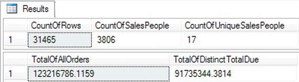
Figure 5-10. Using DISTINCT in an aggregate expression
You can use DISTINCT either to return unique rows from your query or to make your aggregate expression operate on unique values in your data. Practice what you have learned by completing Exercise 5-4.
Aggregate Queries with More Than One Table
So far, the examples have demonstrated how to write aggregate queries involving just one table. You may use aggregate expressions and the GROUP BY and HAVING clauses when joining tables as well; the same rules apply. Type in and execute the code in Listing 5-9 to learn how to do this.
Listing 5-9. Writing Aggregate Queries with Two Tables
USE AdventureWorks2012;

GO


--1

SELECT c.CustomerID, c.AccountNumber, COUNT(*) AS CountOfOrders,

    SUM(TotalDue) AS SumOfTotalDue

FROM Sales.Customer AS c

INNER JOIN Sales.SalesOrderHeader AS s ON c.CustomerID = s.CustomerID

GROUP BY c.CustomerID, c.AccountNumber

ORDER BY c.CustomerID;


--2

SELECT c.CustomerID, c.AccountNumber, COUNT(*) AS CountOfOrders,

    SUM(TotalDue) AS SumOfTotalDue

FROM Sales.Customer AS c

LEFT OUTER JOIN Sales.SalesOrderHeader AS s ON c.CustomerID = s.CustomerID

GROUP BY c.CustomerID, c.AccountNumber

ORDER BY c.CustomerID;


--3

SELECT c.CustomerID, c.AccountNumber,COUNT(s.SalesOrderID) AS CountOfOrders,

    SUM(COALESCE(TotalDue,0)) AS SumOfTotalDue

FROM Sales.Customer AS c

LEFT OUTER JOIN Sales.SalesOrderHeader AS s ON c.CustomerID = s.CustomerID

GROUP BY c.CustomerID, c.AccountNumber

ORDER BY c.CustomerID;
You can see the results of Listing 5-9 in Figure 5-11. All three queries join the Sales.Customer and Sales.SalesOrderHeader tables together and attempt to count the orders placed and calculate the sum of the total due for each customer.

Figure 5-11. The partial results of using aggregates with multiple tables
Using an INNER JOIN, query 1 includes only the customers who have placed an order. By changing to a LEFT OUTER JOIN, query 2 includes all customers but incorrectly returns a count of 1 for customers with no orders and returns a NULL for the SumOfTotalDue when you probably want to see 0. Query 3 solves the first problem by changing COUNT(*) to COUNT(s.SalesOrderID), which eliminates the NULL values and correctly returns 0 for those customers who have not placed an order. Query 3 solves the second problem by using COALESCE to change the NULL value to 0.
Remember that writing aggregate queries with multiple tables is really not different from with just one table; the same rules apply. You can use your knowledge from the previous chapters, such as how to write a WHERE clause and how to join tables to write aggregate queries. Practice what you have learned by completing Exercise 5-5.
Isolating Aggregate Query Logic
Several techniques exist that allow you to separate an aggregate query from the rest of the statement. Sometimes this is necessary because the grouping levels and the columns that must be displayed are not compatible. This section will demonstrate these techniques.
Using a Correlated Subquery in the WHERE Clause
In Chapter 4 you learned how to add subqueries to the WHERE clause. Developers often use another type of subquery, the correlated subquery, to isolate an aggregate query. In a correlated subquery, the subquery refers to the outer query within the subquery’s WHERE clause.
You will likely see this query type used, so I want you to be familiar with it, but other options shown later in the section will be better choices for your own code. Here is the syntax:
SELECT <select list>

FROM <table1>

WHERE <value or column> = (SELECT <aggregate function>(<col1>)

    FROM <table2>

    WHERE <col2> = <table1>.<col3>)
Notice that the predicate in the WHERE clause contains an equal to (=) operator instead of the IN operator. Recall that the subqueries described in the “Using a Subquery in an IN List” section in Chapter 4 require the IN operator because the subquery returns multiple rows. The query compares the value from a column in the outer query to a list of values in the subquery when using the IN operator. When using a correlated subquery, the subquery returns only one value for each row of the outer query, and you can use the other operators, such as equal to. In this case, the query compares a value or column from one row to one value returned by the subquery. Take a look at Listing 5-10, which demonstrates this technique.
Listing 5-10. Using a Correlated Subquery in the WHERE Clause
Use AdventureWorks2012;

GO


--1

SELECT CustomerID, SalesOrderID, TotalDue

FROM Sales.SalesOrderHeader AS soh

WHERE 10 =

    (SELECT COUNT(*)

     FROM Sales.SalesOrderDetail

     WHERE SalesOrderID = soh.SalesOrderID);
--2

SELECT CustomerID, SalesOrderID, TotalDue

FROM Sales.SalesOrderHeader AS soh

WHERE 10000 <

    (SELECT SUM(TotalDue)

     FROM Sales.SalesOrderHeader

     WHERE CustomerID = soh.CustomerID);


--3

SELECT CustomerID

FROM Sales.Customer AS c

WHERE CustomerID > (

    SELECT SUM(TotalDue)

    FROM Sales.SalesOrderHeader

    WHERE CustomerID = c.CustomerID);
You can see the partial results in Figure 5-12. Query 1 displays the Sales.SalesOrderHeader rows where there are ten matching detail rows. Inside the subquery’s WHERE clause, the SalesOrderID from the subquery must match the SalesOrderID from the outer query. Usually when the same column name is used, both must be qualified with the table name or alias. In this case, if the column is not qualified, it refers to the tables in the subquery. Of course, if the subquery contains more than one table, you may have to qualify the column name.

Figure 5-12. A correlated subquery in the WHERE clause
Query 2 displays rows from the Sales.SalesOrderHeader table but only for customers who have the sum of TotalDue greater than 10,000. In this case, the CustomerID from the outer query must equal the CustomerID from the subquery. Query 3 demonstrates how you can compare a column to the results of the aggregate expression in the subquery. The query compares the CustomerID to the sum of the orders and displays the customers who have ordered less than the CustomerID. Of course, this particular example may not make sense from a business rules perspective, but it shows that you can compare a column to the value of an aggregate function using a correlated subquery.
Inline Correlated Subqueries
You may also see correlated subqueries used within the SELECT list. I really don’t recommend this technique because if the query contains more than one correlated subquery, performance deteriorates quickly. You will learn about better options later in this section. Here is the syntax for the inline correlated subquery:
SELECT <select list>,

    (SELECT <aggregate function>(<col1>)

     FROM <table2> WHERE <col2> = <table1>.<col3>) AS <alias name>

FROM <table1>
The subquery must produce only one row for each row of the outer query, and only one expression may be returned from the subquery. Listing 5-11 shows two examples of this query type.
Listing 5-11. Using an Inline Correlated Subquery
USE AdventureWorks2012;

GO


--1

SELECT CustomerID,

    (SELECT COUNT(*)

     FROM Sales.SalesOrderHeader

     WHERE CustomerID = C.CustomerID) AS CountOfSales

FROM Sales.Customer AS C

ORDER BY CountOfSales DESC;


--2

SELECT CustomerID,

    (SELECT COUNT(*) AS CountOfSales

     FROM Sales.SalesOrderHeader

     WHERE CustomerID = C.CustomerID) AS CountOfSales,

    (SELECT SUM(TotalDue)

     FROM Sales.SalesOrderHeader

     WHERE CustomerID = C.CustomerID) AS SumOfTotalDue,

    (SELECT AVG(TotalDue)

     FROM Sales.SalesOrderHeader

     WHERE CustomerID = C.CustomerID) AS AvgOfTotalDue

FROM Sales.Customer AS C

ORDER BY CountOfSales DESC;
You can see the results in Figure 5-13. Query 1 demonstrates how an inline correlated subquery returns one value per row. Notice the WHERE clause in the subquery. The CustomerID column must be equal to the CustomerID in the outer query. The alias for the column must be added right after the subquery definition, not the column definition.

Figure 5-13. Using an inline correlated subquery
Normally, when working with the same column name from two tables, both must be qualified. Within the subquery, if the column is not qualified, the column is assumed to be from the table within the subquery. If the subquery involves multiple tables, well, then you will probably have to qualify the columns.
Notice that Query 2 contains three correlated subqueries because three values are required. Although one correlated subquery doesn’t usually cause a problem, performance quickly deteriorates as additional correlated subqueries are added to the query. Luckily, other techniques exist to get the same results with better performance.
Using Derived Tables
In Chapter 4 you learned about derived tables. You can use derived tables to isolate the aggregate query from the rest of the query, especially when working with SQL Server 2000, without a performance hit. Here is the syntax:
SELECT <col1>,<col4>,<col3> FROM <table1> AS a

INNER JOIN

    (SELECT <aggregate function>(<col2>) AS <col4>,<col3>

     FROM <table2> GROUP BY <col3>) AS b ON a.<col1> = b.<col3>
Listing 5-12 shows how to use this technique. Type in and execute the code.
Listing 5-12. Using a Derived Table
USE AdventureWorks2012;

GO


SELECT c.CustomerID,CountOfSales,

    SumOfTotalDue, AvgOfTotalDue

FROM Sales.Customer AS c INNER JOIN

    (SELECT CustomerID, COUNT(*) AS CountOfSales,
         SUM(TotalDue) AS SumOfTotalDue,

         AVG(TotalDue) AS AvgOfTotalDue

     FROM Sales.SalesOrderHeader

     GROUP BY CustomerID) AS s

ON c.CustomerID = s.CustomerID;
You can see the results in Figure 5-14. This query has much better performance than the second query in Listing 5-11, but it produces the same results. Remember that any column required in the outer query must be listed in the derived table. You must also supply an alias for the derived table.

Figure 5-14. The partial results of using a derived table
Besides the increase in performance, the derived table may return more than one row for each row of the outer query, and multiple aggregates may be included. If you are working with some legacy SQL Server 2000 systems, keep derived tables in mind for solving complicated T-SQL problems.
Common Table Expressions
You learned about common table expressions (CTEs) in Chapter 4. A CTE also allows you to isolate the aggregate query from the rest of the statement. The CTE is not stored as an object; it just makes the data available during the query. Here is the syntax:
WITH <cteName> AS (SELECT <aggregate function>(<col2>) AS <col4>, <col3>

   FROM <table2> GROUP BY <col3>)

SELECT <col1>,<col4>,<col3>

FROM <table1> INNER JOIN b ON <cteName>.<col1> = <table1>.<col3>
Type in and execute the code in Listing 5-13 to learn how to use a CTE with an aggregate query.
Listing 5-13. Using a Common Table Expression
USE AdventureWorks2012;

GO


WITH s AS

    (SELECT CustomerID, COUNT(*) AS CountOfSales,

        SUM(TotalDue) AS SumOfTotalDue,

        AVG(TotalDue) AS AvgOfTotalDue
     FROM Sales.SalesOrderHeader

     GROUP BY CustomerID)

SELECT c.CustomerID,CountOfSales,

    SumOfTotalDue, AvgOfTotalDue

FROM Sales.Customer AS c INNER JOIN s

ON c.CustomerID = s.CustomerID;
Figure 5-15 displays the results. This query looks a lot like the one in Listing 5-12, just rearranged a bit. At this point, there is no real advantage to the CTE over the derived table, but it is easier to read, in my opinion. CTEs have several extra features that you will learn about in Chapter 11.

Figure 5-15. Using a common table expression
Using Derived Tables and CTEs to Display Details
Suppose you want to display several nonaggregated columns along with some aggregate expressions that apply to the entire result set or to a larger grouping level. For example, you may need to display several columns from the Sales.SalesOrderHeader table and calculate the percent of the TotalDue for each sale compared to the TotalDue for all the customer’s sales. If you group by CustomerID, you can’t include other nonaggregated columns from Sales.SalesOrderHeader unless you group by those columns. To get around this, you can use a derived table or a CTE. Type in and execute the code in Listing 5-14 to learn this technique.
Listing 5-14. Displaying Details
USE AdventureWorks2012;

GO


--1

SELECT c.CustomerID, SalesOrderID, TotalDue, AvgOfTotalDue,

    TotalDue/SumOfTotalDue * 100 AS SalePercent

FROM Sales.SalesOrderHeader AS soh

INNER JOIN

    (SELECT CustomerID, SUM(TotalDue) AS SumOfTotalDue,

     AVG(TotalDue) AS AvgOfTotalDue

     FROM Sales.SalesOrderHeader

     GROUP BY CustomerID) AS c ON soh.CustomerID = c.CustomerID

ORDER BY c.CustomerID;
--2

WITH c AS

    (SELECT CustomerID, SUM(TotalDue) AS SumOfTotalDue,

        AVG(TotalDue) AS AvgOfTotalDue

     FROM Sales.SalesOrderHeader

     GROUP BY CustomerID)

SELECT c.CustomerID, SalesOrderID, TotalDue,AvgOfTotalDue,

    TotalDue/SumOfTotalDue * 100 AS SalePercent

FROM Sales.SalesOrderHeader AS soh

INNER JOIN c ON soh.CustomerID = c.CustomerID

ORDER BY c.CustomerID;
Take a look at the results in Figure 5-16. The queries return the same results and just use different techniques. Inside the derived table or CTE, the data is grouped by CustomerID. The outer query contains no grouping at all, and any columns can be used. Either of these techniques performs much better than the equivalent query written with correlated subqueries.

Figure 5-16. The results of displaying details with a derived table and a CTE
The OVER Clause
The OVER clause provides a way to add aggregate values to a nonaggregate query. For example, you may need to write a report that compares the total due of each order to the total due of the average order. The query is not really an aggregate query, but one aggregate value from the entire results set or a grouping level is required to perform the calculation. Here is the syntax:
SELECT <col1>,<aggregate function>(<col2>) OVER([PARTITION BY <col3>])

FROM <table1>
Type in and execute the code in Listing 5-15 to learn how to use OVER.
Listing 5-15. Using the OVER Clause
USE AdventureWorks2012;

GO


SELECT CustomerID, SalesOrderID, TotalDue,

    AVG(TotalDue) OVER(PARTITION BY CustomerID) AS AvgOfTotalDue,

    SUM(TotalDue) OVER(PARTITION BY CustomerID) AS SumOfTOtalDue,

    TotalDue/(SUM(TotalDue) OVER(PARTITION BY CustomerID)) * 100

        AS SalePercentPerCustomer,

    SUM(TotalDue) OVER() AS SalesOverAll

FROM Sales.SalesOrderHeader

ORDER BY CustomerID;
Figure 5-17 displays the results. The PARTITION BY part of the expressions specifies the grouping over which the aggregate is calculated. In this example, when partitioned by CustomerID, the function calculates the value grouped over CustomerID. When no PARTITION BY is specified, as in the SalesOverAll column, the aggregate is calculated over the entire result set.
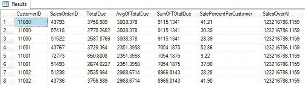
Figure 5-17. Using the OVER clause
You can also include a GROUP BY in the overall query. Be careful here because any columns that are part of the OVER clause aggregate must be grouped. If you need to do this, you are probably better off solving the problem with a CTE.
The OVER clause allows you to add an aggregate function to an otherwise nonaggregate query. Practice using the OVER clause by completing Exercise 5-65.
GROUPING SETS
GROUPING SETS, when added to an aggregate query, allows you to combine different grouping levels within one statement. This is equivalent to combining multiple aggregate queries with UNION. For example, suppose you want the data summarized by one column combined with the data summarized by a different column. Just like MERGE, this feature is very valuable for loading data warehouses and data marts. When using GROUPING SETS instead of UNION, you can see increased performance, especially when the query includes a WHERE clause and the number of columns specified in the GROUPING SETS clause increases. Here is the syntax:
SELECT <col1>,<col2>,<aggregate function>(<col3>)

FROM <table1>

WHERE <criteria>

GROUP BY GROUPING SETS (<col1>,<col2>)
Listing 5-16 compares the equivalent UNION query to a query using GROUPING SETS. Type in and execute the code to learn more.
Listing 5-16. Using GROUPING SETS
USE AdventureWorks2012;

GO


--1

SELECT NULL AS SalesOrderID,SUM(UnitPrice)AS SumOfPrice,ProductID

FROM Sales.SalesOrderDetail

WHERE SalesOrderID BETWEEN 44175 AND 44180

GROUP BY ProductID

UNION

SELECT SalesOrderID,SUM(UnitPrice), NULL

FROM Sales.SalesOrderDetail

WHERE SalesOrderID BETWEEN 44175 AND 44180

GROUP BY SalesOrderID;


--2

SELECT SalesOrderID,SUM(UnitPrice) AS SumOfPrice,ProductID

FROM Sales.SalesOrderDetail

WHERE SalesOrderID BETWEEN 44175 AND 44180

GROUP BY GROUPING SETS(SalesOrderID,ProductID);
Figure 5-18 shows the partial results. Query 1 is a UNION query that calculates the sum of the UnitPrice. The first part of the query supplies a NULL value for SalesOrderID. That is because SalesOrderID is just a placeholder. The query groups by ProductID, and SalesOrderID is not needed. The second part of the query supplies a NULL value for ProductID. In this case, the query groups by SalesOrderID, and ProductID is not needed. The UNION query combines the results. Query 2 demonstrates how to write the equivalent query using GROUPING SETS.
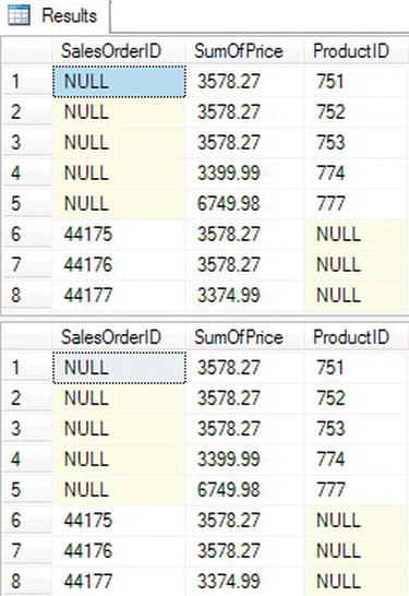
Figure 5-18. The partial results of comparing UNION to GROUPING SETS
CUBE and ROLLUP
You can add subtotals to your aggregate queries by using CUBE or ROLLUP in the GROUP BY clause. CUBE and ROLLUP are very similar, but there is a subtle difference. CUBE will give subtotals for every possible combination of the grouping levels. ROLLUP will give subtotals for the hierarchy. For example, if you are grouping by three columns, CUBE will provide subtotals for every grouping column. ROLLUP will provide subtotals for the first two columns but not the last column in the GROUP BY list. Here is the syntax:
SELECT <col1>, <col2>, <aggregate expression>

     FROM <table>

GROUP BY <CUBE or ROLLUP>(<col1>,<col2>)
The following example demonstrates how to use CUBE and ROLLUP. Run the code in Listing 5-17 to see how this works.
--1

USE AdventureWorks2012

GO

SELECT COUNT(*) AS CountOfRows, Color,

        ISNULL(Size,CASE WHEN GROUPING(Size) = 0 THEN 'UNK' ELSE 'ALL' END) AS Size

FROM Production.Product

GROUP BY CUBE(Color,Size)

ORDER BY Size;


--2

SELECT COUNT(*) AS CountOfRows, Color,

        ISNULL(Size,CASE WHEN GROUPING(Size) = 0 THEN 'UNK' ELSE 'ALL' END) AS Size

FROM Production.Product

GROUP BY ROLLUP(Color,Size)

ORDER BY Size;
Figure 5-19 shows the partial results. Query 1 returns 98 rows while Query 2 returns only 79 rows. Notice that Query 2 doesn’t have an ALL row for size 38. Query 2 returns a subtotal row for every color but not every size. Query 1 returns a subtotal row for every color and every size.
In this example, the subtotal row for Red contains a NULL in the size column. In order to distinguish the subtotal rows from legitimate NULLs in the data, use the GROUPING function. The GROUPING function returns a 1 in the subtotal rows. Combine GROUPING with the ISNULL function to handle this.
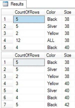
Figure 5-19. The partial results of CUBE and ROLLUP
Thinking About Performance
Inline correlated subqueries are very popular among developers. Unfortunately, the performance is poor compared to other techniques, such as derived tables and CTEs. Toggle on the Include Actual Execution Plan setting before typing and executing the code in Listing 5-18.
Listing 5-18. Comparing a Correlated Subquery to a Common Table Expression
USE AdventureWorks2012;

GO


--1

SELECT CustomerID,

    (SELECT COUNT(*) AS CountOfSales

     FROM Sales.SalesOrderHeader

     WHERE CustomerID = c.CustomerID) AS CountOfSales,

    (SELECT SUM(TotalDue)

     FROM Sales.SalesOrderHeader

     WHERE CustomerID = c.CustomerID) AS SumOfTotalDue,

    (SELECT AVG(TotalDue)

     FROM Sales.SalesOrderHeader

     WHERE CustomerID = c.CustomerID) AS AvgOfTotalDue

FROM Sales.Customer AS c

ORDER BY CountOfSales DESC;


--2

WITH Totals AS

   (SELECT COUNT(*) AS CountOfSales,

        SUM(TotalDue) AS SumOfTotalDue,

        AVG(TotalDue) AS AvgOfTotalDue,

        CustomerID

    FROM Sales.SalesOrderHeader

    GROUP BY CustomerID)

SELECT c.CustomerID, CountOfSales,SumOfTotalDue, AvgOfTotalDue

FROM Totals

LEFT OUTER JOIN Sales.Customer AS c ON Totals.CustomerID = c.CustomerID

ORDER BY CountOfSales DESC;
Figure 5-20 displays a portion of the execution plan windows. These plans are pretty complex, but the important thing to note is that query 1, with the correlated subqueries, takes up 62 percent of the resources. Query 2, with the CTE, produces the same results but requires only 38 percent of the resources.

Figure 5-20. The execution plans when comparing a derived table to a CTE
As you can see, the way you write a query can often have a big impact on the performance. Complete Exercise 5-7 to learn more about the performance of aggregate queries.
Summary
If you follow the steps outlined in the preceding sections, you will be able to write aggregate queries. With practice, you will become proficient. Keep the following rules in mind when writing an aggregate query:
- Any column not contained in an aggregate function in the
SELECTlist orORDER BYclause must be part of theGROUP BYclause.- Once an aggregate function, the
GROUP BYclause, or theHAVINGclause appears in a query, it is an aggregate query.- Use the
WHEREclause to filter out rows before the grouping and aggregates are applied. TheWHEREclause doesn’t allow aggregate functions.- Use the
HAVINGclause to filter out rows using aggregate functions.- Don’t include anything in the
SELECTlist orORDER BYclause that you don’t want as a grouping level.- Use common table expressions or derived tables instead of correlated subqueries to solve tricky aggregate query problems.
- To combine more than one grouping combination, use
GROUPING SETS.- Use
CUBEandROLLUPto produce subtotal rows.- Remember that aggregate functions ignore
NULLvalues except forCOUNT(*).