
Chapter 10
Exposing Exponential and Logarithmic Functions
IN THIS CHAPTER
![]() Getting comfortable with exponential expressions
Getting comfortable with exponential expressions
![]() Functioning with base b and base e
Functioning with base b and base e
![]() Taming exponential equations and compound interest
Taming exponential equations and compound interest
![]() Working with logarithmic functions
Working with logarithmic functions
![]() Rolling over on log equations
Rolling over on log equations
![]() Picturing exponentials and logs
Picturing exponentials and logs
Exponential growth and decay are natural phenomena. They happen all around us. And, being the thorough, worldly people they are, mathematicians have come up with ways of describing, formulating, and graphing these phenomena. You express the patterns observed when exponential growth and decay occur mathematically with exponential and logarithmic functions.
Why else are these functions important? Certain algebraic functions, such as polynomials and rational functions, share certain characteristics that exponential functions lack. For example, algebraic functions all show their variables as bases raised to some power, such as ![]() or
or ![]() . Exponential functions, on the other hand, show their variables up in the powers of the expressions and lower some numbers as the bases, such as
. Exponential functions, on the other hand, show their variables up in the powers of the expressions and lower some numbers as the bases, such as ![]() or
or ![]() . In this chapter, I discuss the properties, uses, and graphs of exponential and logarithmic functions in detail.
. In this chapter, I discuss the properties, uses, and graphs of exponential and logarithmic functions in detail.
Evaluating Exponential Expressions
An exponential function is unique because its variable appears in the exponential position and its constant appears in the base position. You write an exponent, or power, as a superscript just after the base. In the expression ![]() , for example, the variable x is the exponent, and the constant 3 is the base. The general form for an exponential function is
, for example, the variable x is the exponent, and the constant 3 is the base. The general form for an exponential function is ![]() , where
, where
- The base b is any positive number.
- The coefficients a and k are any real numbers.
- The exponent x is any real number.
The base of an exponential function can’t be zero or negative; the domain is all real numbers; and the range is all positive numbers when a is positive (see Chapter 6 for more on these topics).
When you enter a number into an exponential function, you evaluate it by using the order of operations (along with other rules for working with exponents; I discuss these topics in Chapters 1 and 4). The order of operations dictates that you evaluate the function in the following order:
- Powers and roots
- Multiplication and division
- Addition and subtraction
If you want to evaluate ![]() for
for ![]() , for example, you replace the x with the number 2. So,
, for example, you replace the x with the number 2. So, ![]() . To evaluate the exponential function
. To evaluate the exponential function ![]() for
for ![]() , you write the steps as follows:
, you write the steps as follows:

You raise to the power first, after flipping the fraction to get rid of the negative sign, and then multiply by 4, and finally subtract 3.
Exponential Functions: It’s All about the Base, Baby
The base of an exponential function can be any positive number. The bigger the number, the bigger the function value becomes as you raise it to higher and higher powers. (Sort of like the more money you have, the more money you make.) The bases can get downright small, too. In fact, when the base is some number between zero and one, you don’t have a function that grows; instead, you have a function that falls.
Observing the trends in bases
The base of an exponential function tells you so much about the nature and character of the function, making it one of the first things you should look at and classify. The main way to classify the bases of exponential functions is to determine whether they’re larger or smaller than one. After you make that designation, you look at how much larger or how much smaller. The exponents themselves affect the expressions that contain them in somewhat predictable ways, making them prime places to look when grouping.
 Because the domain (or input; see Chapter 6) of exponential functions is all real numbers, and the base is always positive, the result of
 ![]() is always a positive number. Even when you raise a positive base to a negative power, you get a positive answer. Exponential functions can end up with negative values if you subtract from the power or multiply by a negative number, but the power itself is always positive.
is always a positive number. Even when you raise a positive base to a negative power, you get a positive answer. Exponential functions can end up with negative values if you subtract from the power or multiply by a negative number, but the power itself is always positive.
Grouping exponential functions according to their bases
Algebra offers three classifications for the base of an exponential function, due to the fact that the numbers used as bases appear to react in distinctive ways when raised to positive powers:
- When
 , the values of
  grow larger as x gets bigger — for instance,
  ,
,  , and so on.
 When
 , the values of
  show no movement. Raising the number 1 to higher powers always results in the number
  ,
,  ,
,  , and so on. You see no exponential growth or decay.
 In fact, some mathematicians leave the number 1 out of the listing of possible bases for exponentials. Others leave it in as a bridge between functions that increase in value and those that decrease in value. It’s just a matter of personal taste.
- When
 , the value of
  grows smaller as x gets bigger. The base b has to be positive, and the numbers
  are all proper fractions (fractions with the numerators smaller than the denominators). Look at what happens to a fractional base when you raise it to the second, fifth, and eighth degrees:
 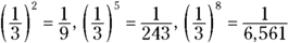 . The numbers get smaller and smaller as the powers get bigger.
Adding a coefficient of k to the exponent (making it kx) can change the behavior of the function, depending on what sign k is. After you take into account the effect of multiplying by k, though, the basic properties remain the same.
Grouping exponential functions according to their exponents
An exponent placed with a number can affect the expression that contains the number in somewhat predictable ways. The exponent makes the result take on different qualities, depending on whether the exponent is greater than zero, equal to zero, or smaller than zero:
- When the base
 and the exponent
  , the values of
  get bigger and bigger as x gets larger — for instance,
  and
and  . You say that the values grow exponentially.
 - When the base
 and the exponent
  , the only value of
  you get is 1. The rule is that
  for any number except
  . So, an exponent of zero really flattens things out.
 - When the base
 and the exponent
  — a negative number — the values of
  get smaller and smaller as the exponents get further and further from zero. Take these expressions, for example:
  and
and  . These numbers can get very small very quickly.
Meeting the most frequently used bases: 10 and e
Exponential functions feature bases represented by numbers greater than zero. The two most frequently used bases are 10 and e, where ![]() and
and ![]() .
.
It isn’t too hard to understand why mathematicians like to use base 10 — in fact, just hold all your fingers in front of your face! All the powers of 10 are made up of ones and zeros — for instance, ![]() , and
, and ![]() . How much more simple can it get? Our number system, the decimal system, is based on tens.
. How much more simple can it get? Our number system, the decimal system, is based on tens.
Like the value 10, base e occurs naturally. Members of the scientific world prefer base e because powers and multiples of e keep creeping up in models of natural occurrences. Including e’s in computations also simplifies things for financial professionals, mathematicians, and engineers.
If you use a scientific calculator to get the value of e, you see only some of e. The numbers you see estimate only what e is; most calculators give you seven or eight decimal places. Here are the first nine decimal places in the value of e, in rounded form:
The decimal value of e actually goes on forever without repeating in a pattern. The hint of a pattern you see in the nine digits doesn’t hold for long.
The expression ![]() represents the exact value of e. The larger and larger x gets, the more correct decimal places you get. Most algebra courses call for you to memorize only the first four digits of e: 2.718.
represents the exact value of e. The larger and larger x gets, the more correct decimal places you get. Most algebra courses call for you to memorize only the first four digits of e: 2.718.
Now for the bad news. As wonderful as e is for taming function equations and scientific formulas, its powers aren’t particularly easy to deal with. The base e is approximately 2.718, and when you take a number with a decimal value that never ends and raise it to a power, the decimal values get even more unwieldy. The common practice in mathematics is to leave your answers as multiples and powers of e instead of switching to decimals, unless you need an approximation in some application. Scientific calculators change your final answer, in terms of e, to an answer correct to as many decimal places as needed.
 You follow the same rules when simplifying an expression that has a factor of e that you use on a variable base (see Chapter 4). The following list presents some examples of how you simplify expressions with a base of e:
- When you multiply expressions with the same base, you add the exponents:

- When you divide expressions with the same base, you subtract the exponents:

- The two exponents don’t combine any further.
- Use the order of operations — powers first, followed by multiplication, addition, or subtraction:

- Change radicals to fractional exponents:

Solving Exponential Equations
To solve an algebraic equation, you work toward finding the numbers that replace any variables and make a true statement. The process of solving exponential equations incorporates many of the same techniques you use in algebraic equations — adding to or subtracting from each side, multiplying or dividing each side by the same number, factoring, squaring both sides, and so on.
Solving exponential equations requires some additional techniques, however. That’s what makes them so much fun! Some techniques you use when solving exponential equations involve changing the original exponential equations into new equations that have matching bases. Other techniques involve putting the exponential equations into more recognizable forms — such as quadratic equations — and then using the appropriate formulas. (If you can’t change the bases to matching bases or put the equations into quadratic or linear forms, you have to switch to logarithms or use a change-of-base formula — neither of which is within the scope of this book.)
Making bases match
If you have an equation written in the form ![]() , where the same number represents the bases b, the following rule holds:
, where the same number represents the bases b, the following rule holds:
You read the rule as follows: “If b raised to the xth power is equal to b raised to the yth power, that implies that ![]() .” The double-pointed arrow indicates that the rule is true in the opposite direction, too.
.” The double-pointed arrow indicates that the rule is true in the opposite direction, too.
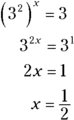
Using the base rule to solve the equation ![]() , you see that the bases (the 2’s) are the same, so the exponents must also be the same. You just pull the exponents down and solve the linear equation
, you see that the bases (the 2’s) are the same, so the exponents must also be the same. You just pull the exponents down and solve the linear equation ![]() for the value of
for the value of ![]() , or
, or ![]() . You then put the 4 back into the original equation to check your answer:
. You then put the 4 back into the original equation to check your answer: ![]() , which simplifies to
, which simplifies to ![]() , or
, or ![]() .
.
Seems simple enough. But what do you do if the bases aren’t the same? Unfortunately, if you can’t change the problem to make the bases the same, you can’t solve the problem with this rule. (In this case, you either use logarithms — change to a logarithmic equation — or resort to technology.)
When bases are related
Many times, bases are related to one another by being powers of the same number.
For example, to solve the equation ![]() , you need to write both the bases as powers of 2 and then apply the rules of exponents (see Chapter 4). Here are the steps of the solution:
, you need to write both the bases as powers of 2 and then apply the rules of exponents (see Chapter 4). Here are the steps of the solution:
- Change the 4 and 8 to powers of 2.

- Raise a power to a power.

- Equate the two exponents, because the bases are now the same, and then solve for x.

- Check your answer in the original equation.

When other operations are involved
Changing all the bases in an equation to a single base is especially helpful when you have operations such as roots, multiplication, or division involved.
If you want to solve the equation ![]() for x, for example, your best approach is to change each of the bases to a power of 3 and then apply the rules of exponents (see Chapter 4).
for x, for example, your best approach is to change each of the bases to a power of 3 and then apply the rules of exponents (see Chapter 4).
Here’s how you change the bases and powers in the example equation (Steps 1 and 2 from the list in the previous section): You change the bases 9 and 27 to powers of 3, replace the radical with a fractional exponent, and then raise the powers to other powers by multiplying the exponents.

When you divide two numbers with the same base, you subtract the exponents. After you have a single power of 3 on each side, you can equate the exponents and solve for x:

Recognizing and using quadratic patterns
When exponential terms appear in equations with two or three terms, you may be able to treat the equations as you do quadratic equations (see Chapter 3) to solve them with familiar methods. Using the methods for solving quadratic equations is a big advantage because you can factor the exponential equations, or you can resort to the quadratic formula.
You factor quadratics by dividing every term by a common factor or, with trinomials, by using unFOIL to determine the two binomials whose product is the trinomial. (Refer to Chapters 1 and 3 if you need a refresher on these types of factoring.)
You can make use of just about any equation pattern that you see when solving exponential functions. If you can simplify the exponential to the form of a quadratic or cubic and then factor, find perfect squares, find sums and differences of squares, and so on, you’ve made life easier by changing the equation into something recognizable and doable. In the sections that follow, I provide examples of the two most common types of problems you’re likely to run up against: those involving common factors and unFOIL.
Taking out a greatest common factor
When you solve a quadratic equation by factoring out a greatest common factor (GCF), you write that greatest common factor outside the parentheses and show all the results of dividing by it inside the parentheses.
In the equation ![]() , for example, you factor
, for example, you factor ![]() from each term and get
from each term and get ![]() . After factoring, you use the multiplication property of zero by setting each of the separate factors equal to zero. (If the product of two numbers is zero, at least one of the numbers must be zero; see Chapter 1.) You set the factors equal to zero to find out what x satisfies the equation:
. After factoring, you use the multiplication property of zero by setting each of the separate factors equal to zero. (If the product of two numbers is zero, at least one of the numbers must be zero; see Chapter 1.) You set the factors equal to zero to find out what x satisfies the equation:
has no solution; 3 raised to a power can’t be equal to 0.
Setting ![]() , you change the 9 to a power of 3 to get
, you change the 9 to a power of 3 to get ![]() . Move the
. Move the ![]() to the right, and the equation becomes
to the right, and the equation becomes ![]() . Setting the exponents equal to one another,
. Setting the exponents equal to one another, ![]() . You find only one solution to the entire equation.
. You find only one solution to the entire equation.
Factoring like a quadratic trinomial
A quadratic trinomial has a term with the variable squared, a term with the variable raised to the first power, and a constant term. This is the pattern you’re looking for if you want to solve an exponential equation by treating it like a quadratic. The trinomial ![]() , for example, resembles a quadratic trinomial that you can factor. One option is to consider the quadratic
, for example, resembles a quadratic trinomial that you can factor. One option is to consider the quadratic ![]() , which would look something like the exponential equation if you replace each
, which would look something like the exponential equation if you replace each ![]() with a y. The quadratic in y’s factors into
with a y. The quadratic in y’s factors into ![]() . Using the same pattern on the exponential version, you get the factorization
. Using the same pattern on the exponential version, you get the factorization ![]() . Setting each factor equal to zero, when
. Setting each factor equal to zero, when ![]() ,
, ![]() . This equation holds true when
. This equation holds true when ![]() , making that one of the solutions. Now, when
, making that one of the solutions. Now, when ![]() , you say that
, you say that ![]() , or
, or ![]() . In other words,
. In other words, ![]() . You find two solutions to this equation:
. You find two solutions to this equation: ![]() and
and ![]() .
.
Showing an “Interest” in Exponential Functions
Professionals (you included, although you may not know it) use exponential functions in many financial applications. If you have a mortgage on your home, an annuity for your retirement, or a credit-card balance, you should be interested in interest — and in the exponential functions that drive it.
Applying the compound interest formula
When you deposit your money in a savings account, an individual retirement account (IRA), or other investment vehicle, you get paid for the money you invest; this payment comes from the proceeds of compound interest — interest that earns interest. For instance, if you invest $100 and earn $2 in interest, the two amounts come together, and you now earn interest on $102. The interest compounds. This, of course, is a wonderful thing.
Here’s the formula you can use to determine the total amount of money you have (A) after you deposit the principal (P) that earns interest at the rate of r percent (written as a decimal), compounding n times each year for t years:
For example, say you receive a windfall of $20,000 for an unexpected inheritance, and you want to sock it away for 10 years. You invest the cash in a fund at 4.5 percent interest (if you’re lucky enough to find something that good), compounded monthly. How much money will you have at the end of 10 years if you can manage to keep your hands off it? Apply the formula as follows:

You’d have over $31,300. This growth in your money shows you the power of compounding and exponents.
Planning on the future: Target sums
You can figure out what amount of money you’ll have in the future if you make a certain deposit now by applying the compound interest formula. But how about going in the opposite direction? Can you figure out how much you need to deposit in an account in order to have a target sum in a certain number of years? You sure can.
If you want to have $100,000 available 18 years from now, when your baby will be starting college, how much do you have to deposit in an account that earns 5 percent interest, compounded monthly? To find out, you take the compound interest formula and work backward. This time you’ll be solving for the principal (P):

You solve for P in the equation by dividing each side by the value in the parentheses raised to the power 216. According to the order of operations (see Chapter 1), you raise to a power before you multiply or divide. So, after you set up the division to solve for P, you raise what’s in the parentheses to the 216th power and divide the result into 100,000:

A deposit of almost $41,000 will result in enough money to pay for college in 18 years (not taking into account the escalation of tuition fees). You may want to start talking to your baby about scholarships now !
If you have a target amount of money in mind and want to know how many years it will take to get to that level, you can use the formula for compound interest and work backward. Put in all the specifics — principal, rate, compounding time, the amount you want — and solve for t. You may need a scientific calculator and some logarithms to finish it out, but you’ll do whatever it takes to plan ahead, right?
Measuring the actual compound: Effective rates
When you go into a bank or credit union, you see all sorts of interest rates posted. You may have noticed the words “nominal rate” and “effective rate” in previous visits. The nominal rate is the named rate, or the value entered into the compounding formula. The named rate may be 4 percent or 7.5 percent, but that value isn’t indicative of what’s really happening because of the compounding. The effective rate represents what’s really happening to your money after it compounds. A nominal rate of 4 percent translates into an effective rate of 4.074 percent when compounded monthly. This may not seem like much of a difference — the effective rate is about 0.07 higher — but it makes a big difference if you’re talking about fairly large sums of money or long time periods.
You compute the effective rate by using the middle portion of the compound interest formula: ![]() . To determine the effective rate of 4 percent compounded monthly, for example, you use
. To determine the effective rate of 4 percent compounded monthly, for example, you use ![]() .
.
The 1 before the decimal point in the answer indicates the original amount. You subtract that 1, and the rest of the decimals are the percentage values used for the effective rate.
Table 10-1 shows what happens to a nominal rate of 4 percent when you compound it different numbers of times per year.
TABLE 10-1 Compounding a Nominal 4 Percent Interest Rate
Times Compounded |
Computation |
Effective Rate |
Annually |
|
4.00% |
Biannually |
|
4.04% |
Quarterly |
|
4.06% |
Monthly |
|
4.07% |
Daily |
|
4.08% |
Hourly |
|
4.08% |
Every second |
|
4.08% |
Looking at continuous compounding
Typical compounding of interest occurs annually, quarterly, monthly, or perhaps even daily. Continuous compounding occurs immeasurably quickly or often. To accomplish continuous compounding, you use a different formula than you use for other compounding problems.
Here’s the formula you use to determine a total amount (A) when the initial value or principal is P and when the amount grows continuously at the rate of r percent (written as a decimal) for t years:
The e represents a constant number (the e base; see the section “Meeting the most frequently used bases: 10 and e” earlier in this chapter) — approximately 2.71828. You can use this formula to determine how much money you’d have after 10 years of investment, for example, when the interest rate is 4.5 percent and you deposit $20,000:
You should use the continuous compounding formula as an approximation in appropriate situations — when you’re not actually paying out the money. The compound interest formula is much easier to deal with and gives a good estimate of total value.
Using the continuous compounding formula to approximate the effective rate of 4 percent compounded continuously, you get ![]() (an effective rate of 4.08 percent). Compare this with the value in Table 10-1 in the previous section.
(an effective rate of 4.08 percent). Compare this with the value in Table 10-1 in the previous section.
Logging On to Logarithmic Functions
A logarithm is the exponent of a number. Logarithmic (log) functions are the inverses of exponential functions. They answer the question, “What power gave me that answer?” The log function associated with the exponential function ![]() , for example, is
, for example, is ![]() . The superscript
. The superscript ![]() after the function name f indicates that you’re looking at the inverse of the function f. So,
after the function name f indicates that you’re looking at the inverse of the function f. So, ![]() , for example, asks, “What power of 2 gave me 8?”
, for example, asks, “What power of 2 gave me 8?”
A logarithmic function has a base and an argument. The logarithmic function ![]() has a base b and an argument x. The base must always be a positive number and not equal to one. The argument must always be positive.
has a base b and an argument x. The base must always be a positive number and not equal to one. The argument must always be positive.
You can see how a function and its inverse work as exponential and log functions by evaluating the exponential function for a particular value and then seeing how you get that value back after applying the inverse function to the answer. For example, first let ![]() in
in ![]() ; you get
; you get ![]() . You put the answer, 8, into the inverse function
. You put the answer, 8, into the inverse function ![]() , and you get
, and you get ![]() . The answer comes from the definition of how logarithms work; the 2 raised to the power of 3 equals 8. You have the answer to the fundamental logarithmic question, “What power of 2 gave me 8?”
. The answer comes from the definition of how logarithms work; the 2 raised to the power of 3 equals 8. You have the answer to the fundamental logarithmic question, “What power of 2 gave me 8?”
Meeting the properties of logarithms
Logarithmic functions share similar properties with their exponential counterparts. When necessary, the properties of logarithms allow you to manipulate log expressions so you can solve equations or simplify terms. As with exponential functions, the base b of a log function has to be positive. I show the properties of logarithms in Table 10-2.
TABLE 10-2 Properties of Logarithms
Property Name |
Property Rule |
Example |
Equivalence |
|
|
Log of a product |
|
|
Log of a quotient |
|
|
Log of a power |
|
|
Log of 1 |
|
|
Log of the base |
|
|
Exponential terms that have a base e (see the section “Meeting the most frequently used bases: 10 and e”) have special logarithms just for the e’s (the ease?). Instead of writing the log base e as ![]() , you insert a special symbol, ln, for the log. The symbol ln is called the natural logarithm, and it designates that the base is e. The equivalences for base e and the properties of natural logarithms are the same, but they look just a bit different. Table 10-3 shows them.
, you insert a special symbol, ln, for the log. The symbol ln is called the natural logarithm, and it designates that the base is e. The equivalences for base e and the properties of natural logarithms are the same, but they look just a bit different. Table 10-3 shows them.
TABLE 10-3 Properties of Natural Logarithms
Property Name |
Property Rule |
Example |
Equivalence |
|
|
Natural log of a product |
|
|
Natural log of a quotient |
|
|
Natural log of a power |
|
|
Natural log of 1 |
|
|
Natural log of e |
|
|
As you can see in Table 10-3, the natural logs are much easier to write — you have no subscripts. Professionals use natural logs extensively in mathematical, scientific, and engineering applications.
Putting your logs to work
You can use the basic exponential/logarithmic equivalence ![]() to simplify equations that involve logarithms. Applying the equivalence makes the equation much nicer. If you’re asked to evaluate
to simplify equations that involve logarithms. Applying the equivalence makes the equation much nicer. If you’re asked to evaluate ![]() , for example (or if you have to change it into another form), you can write it as an equation,
, for example (or if you have to change it into another form), you can write it as an equation, ![]() , and use the equivalence:
, and use the equivalence: ![]() . Now you have it in a form that you can solve for x (the x that you get is the answer or value of the original expression). You solve by changing the 9 to a power of 3 and then finding x in the new, more familiar form:
. Now you have it in a form that you can solve for x (the x that you get is the answer or value of the original expression). You solve by changing the 9 to a power of 3 and then finding x in the new, more familiar form:
The result tells you that ![]() — much simpler than the original log expression. (If you need to review solving exponential equations, refer to the section “Making bases match” earlier in this chapter.)
— much simpler than the original log expression. (If you need to review solving exponential equations, refer to the section “Making bases match” earlier in this chapter.)
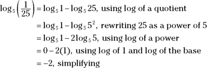
Now look at the process of determining that ![]() is equal to 30. You have to admit that the number 30 is much easier to understand and deal with than
is equal to 30. You have to admit that the number 30 is much easier to understand and deal with than ![]() , so here are the steps:
, so here are the steps:
- Replace
 with x to get
  .
. Simplify
 by first writing 27 as a power of 3.
 , so
, so 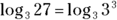 .
.- Use the laws of logarithms involving log of a power and log of a base.

- So if
 , then
  or
or  .
.
As you can see from the preceding equivalence example, the properties of log functions allow you to do simplifications that you just can’t do with other types of functions. For example, because ![]() , you can replace
, you can replace ![]() with the number 1.
with the number 1.
 Using the rules for the log of 1, the log of the base, the log of a power, and the log of a quotient (see Table 10-2), you can change a complicated log expression into something equal to
 ![]() , for example:
, for example:
Expanding expressions with log notation
You write logarithmic expressions and create logarithmic functions by combining all the usual algebraic operations of addition, subtraction, multiplication, division, powers, and roots. Expressions with two or more of these operations can get pretty complicated. A big advantage of logs, though, is their properties. Because of the special features of log properties, you can change multiplication to addition and powers to products. Put all the log properties together, and you can change a single complicated expression into several simpler terms.
If you want to simplify ![]() by using the properties of logarithms, for example, you first use the property for the log of a quotient and then use the property for the log of a product on the first term you get (see Table 10-2 to review these properties):
by using the properties of logarithms, for example, you first use the property for the log of a quotient and then use the property for the log of a product on the first term you get (see Table 10-2 to review these properties):

The last step is to use the log of a power on each term, changing the radical to a fractional exponent first:

The three new terms you create are each much simpler than the original expression.
Rewriting for compactness
Results of computations in science and mathematics can involve sums and differences of logarithms. When this happens, experts usually prefer to have the answers written all in one term, which is where the properties of logarithms come in. You apply the properties in just the opposite way that you break down expressions for greater simplicity (see the previous section). Instead of spreading the work out, you want to create one compact, complicated expression.
To simplify ![]() , for example, you first apply the property involving the natural log (ln) of a power to all three terms (see the section “Meeting the properties of logarithms”). You then factor out
, for example, you first apply the property involving the natural log (ln) of a power to all three terms (see the section “Meeting the properties of logarithms”). You then factor out ![]() from the last two terms and write them in a bracket:
from the last two terms and write them in a bracket:

You now use the property involving the ln of a product on the terms in the bracket, change the ![]() exponent to a radical, and use the property for the ln of a quotient to write everything as the ln of one big fraction:
exponent to a radical, and use the property for the ln of a quotient to write everything as the ln of one big fraction:

The expression is messy and complicated, but it sure is compact.
Solving Logarithmic Equations
Logarithmic equations can have one or more solutions, just like many other types of algebraic equations. What makes solving log equations a bit different is that you get rid of the log part as quickly as possible, leaving you to solve either a polynomial or an exponential equation in its place. Polynomial and exponential equations are easier and more familiar, and you may already know how to solve them (if not, see Chapter 8 and the section “Solving Exponential Equations” earlier in this chapter).
 The only caution I present before you begin solving logarithmic equations is that you need to check the answers you get from the new, revised forms. You may get answers to the polynomial or exponential equations, but they may not work in the original logarithmic equation. Switching to another type of equation introduces the possibility of extraneous roots — answers that fit the new, revised equation that you choose but sometimes don’t fit in with the original equation.
Setting log equal to log
One type of log equation features each term carrying a logarithm in it (all the logarithms have to have the same base). You need to have exactly one log term on each side, so if an equation has more, you apply any properties of logarithms that form the equation to fit the rule (see Table 10-2 for these properties). After you do, you can apply the following rule:
If
, then
When presented with the equation ![]() , for example, you apply this rule so that you can write and solve the equation
, for example, you apply this rule so that you can write and solve the equation ![]() by first setting it equal to 0 and then factoring:
by first setting it equal to 0 and then factoring:

The ![]() and
and ![]() you find are solutions of the quadratic equation, but you must check to see if they work in the original logarithmic equation:
you find are solutions of the quadratic equation, but you must check to see if they work in the original logarithmic equation:
If
 :
:
So, 3 is a solution.
If
 :
:
You have another winner.
When no log base is shown, you assume that the log’s base is 10. Base 10 logarithms are common logarithms.
The following equation shows you how you may get an extraneous solution.
When solving ![]() , you first apply the property involving the log of a product to get just one log term on the left:
, you first apply the property involving the log of a product to get just one log term on the left: ![]() . Next, you use the property that allows you to drop the logs and get the equation
. Next, you use the property that allows you to drop the logs and get the equation ![]() . This is a quadratic equation that you can solve by multiplying, setting it equal to 0, and then factoring (see Chapters 1 and 3):
. This is a quadratic equation that you can solve by multiplying, setting it equal to 0, and then factoring (see Chapters 1 and 3):

Checking the answers, you see that the solution 9 works just fine:

However, the solution ![]() doesn’t work:
doesn’t work:
You can stop right there. Both of the logs on the left have negative arguments. The argument in a logarithm has to be positive, so letting ![]() doesn’t work in the log equation (even though it was just fine in the quadratic equation). You determine that
doesn’t work in the log equation (even though it was just fine in the quadratic equation). You determine that ![]() is an extraneous solution.
is an extraneous solution.
Rewriting log equations as exponentials
When a log equation has log terms as well as a term that doesn’t have a logarithm in it, you need to use algebra techniques and log properties (see Table 10-2) to put the equation in the form ![]() . After you create the right form, you can apply the equivalence to change it to a purely exponential equation.
. After you create the right form, you can apply the equivalence to change it to a purely exponential equation.
For instance, to solve ![]() , you first subtract
, you first subtract ![]() from each side and add 2 to each side to get
from each side and add 2 to each side to get ![]() . Now you apply the property involving the log of a quotient:
. Now you apply the property involving the log of a quotient: ![]() . And then rewrite the equation by using the equivalence and solve for x.
. And then rewrite the equation by using the equivalence and solve for x.

The only solution is ![]() , which works in the original logarithmic equation:
, which works in the original logarithmic equation:

Graphing Exponential and Logarithmic Functions
Exponential and logarithmic functions have rather distinctive graphs because they’re so plain and simple. The graphs are lazy C’s that can slope upward or downward. The main trick when graphing them is to determine any intercepts, which way the graphs move as you go from left to right, and how steep the curves are.
Expounding on the exponential
Exponential functions have curves that usually look like the graphs you see in Figures 10-1a and 10-1b.

John Wiley & Sons, Inc.
FIGURE 10-1: Exponential graphs rise away from the x-axis or fall toward the x-axis.
The graph in Figure 10-1a depicts exponential growth — when the values of the function are increasing. Figure 10-1b depicts exponential decay — when the values of the function are decreasing. Both graphs intersect the y-axis but not the x-axis, and they both have a horizontal asymptote: the x-axis.
Identifying a rise or fall
You can tell whether a graph will feature exponential growth or decay by looking at the equation of the function.
In order to determine whether a function represents exponential growth or decay, you look at its base:
- If the exponential function
 has a base
  , the graph of the function rises as you read from left to right, meaning you observe exponential growth.
 - If the exponential function
 has a base
  , the graph falls as you read from left to right, meaning you observe exponential decay.
The values of the functions ![]() and
and ![]() , for example, both rise as you read from left to right because their bases are greater than 1. The graphs of
, for example, both rise as you read from left to right because their bases are greater than 1. The graphs of ![]() and
and ![]() both fall as you look at increasing values of x, because 0.2 and 0.9 are both between 0 and 1.
both fall as you look at increasing values of x, because 0.2 and 0.9 are both between 0 and 1.
Sketching exponential graphs
In general, exponential functions have no x-intercepts, but they do have single y-intercepts. The exception to this rule is when you change the function equation by subtracting a number from the exponential term; this action drops the curve down below the x-axis.
To find the y-intercept of an exponential function, you set ![]() and solve for y. If you want to find the y-intercept of
and solve for y. If you want to find the y-intercept of ![]() , for example, you replace x with 0 to get
, for example, you replace x with 0 to get ![]() . So, the y-intercept is (0, 3). This function rises from left to right because the base is greater than one. The multiplier 0.4 on the x in the exponent acts like the slope of a line — in this case, making the graph rise more slowly or gently (see Chapter 2).
. So, the y-intercept is (0, 3). This function rises from left to right because the base is greater than one. The multiplier 0.4 on the x in the exponent acts like the slope of a line — in this case, making the graph rise more slowly or gently (see Chapter 2).
Before you try to graph an equation, you should find another point or two for help with the shape. For instance, if ![]() in the previous example,
in the previous example, ![]() . So, the point (5, 12) falls on the curve. Also, if
. So, the point (5, 12) falls on the curve. Also, if ![]() ,
, ![]() (see Chapter 4 for info on dealing with negative exponents). The point
(see Chapter 4 for info on dealing with negative exponents). The point ![]() is also on the curve. Figure 10-2 shows the graph of this example curve with the intercept and points drawn in.
is also on the curve. Figure 10-2 shows the graph of this example curve with the intercept and points drawn in.

John Wiley & Sons, Inc.
FIGURE 10-2: The graph of the exponential function  .
.
To graph the function ![]() , you first find the y-intercept. When
, you first find the y-intercept. When ![]() ,
, ![]() . So, the y-intercept is (0, 10). Two other points you may decide to use are (1, 9) and
. So, the y-intercept is (0, 10). Two other points you may decide to use are (1, 9) and ![]() . The graph of this function falls as you read from left to right because the base is smaller than one. Figure 10-3 shows the graph of this example curve and the random points of reference.
. The graph of this function falls as you read from left to right because the base is smaller than one. Figure 10-3 shows the graph of this example curve and the random points of reference.

John Wiley & Sons, Inc.
FIGURE 10-3: The graph of the exponential function  .
.
Not seeing the logs for the trees
The graphs of logarithmic functions either rise or fall, and they usually look like one of the sketches in Figure 10-4. The graphs have a single vertical asymptote: the y-axis. Having the y-axis as an asymptote is the opposite of an exponential function, whose asymptote is the x-axis (see the previous section). Log functions are also different from exponential functions in that they have an x-intercept but not (usually) a y-intercept.

John Wiley & Sons, Inc.
FIGURE 10-4: Logarithmic functions rise or fall, breaking away from the asymptote: the y-axis.
Graphing log functions with the use of intercepts
When you graph a log function, you look at its x-intercept and the base of the function:
- If the base is a number greater than one, the graph rises from left to right.
- If the base is between zero and one, the graph falls as you go from left to right.
For instance, the graph of ![]() has an x-intercept of (1, 0) and rises from left to right. You get the intercept by letting
has an x-intercept of (1, 0) and rises from left to right. You get the intercept by letting ![]() and solving the equation
and solving the equation ![]() for x. You should choose a couple other points on the curve to help with shaping the graph. The graph of
for x. You should choose a couple other points on the curve to help with shaping the graph. The graph of ![]() contains the points (2, 1) and
contains the points (2, 1) and ![]() . You compute those points by substituting the chosen x value into the function equation and solving for y. (If you need a refresher on how to solve those equations, refer to the section “Solving Logarithmic Equations.”) Figure 10-5 shows you the graph of the example function (the points are indicated).
. You compute those points by substituting the chosen x value into the function equation and solving for y. (If you need a refresher on how to solve those equations, refer to the section “Solving Logarithmic Equations.”) Figure 10-5 shows you the graph of the example function (the points are indicated).

John Wiley & Sons, Inc.
FIGURE 10-5: With a log base of 2, the curve of the function rises.
Reflecting on inverses of exponential functions
Exponential and logarithmic functions are inverses of one another. You may have noticed in previous sections that the flattened, C-shaped curves of log functions look vaguely familiar. In fact, they’re mirror images of the graphs of exponential functions.
An exponential function, ![]() , and its logarithmic inverse,
, and its logarithmic inverse, ![]() , have graphs that mirror one another over the line
, have graphs that mirror one another over the line ![]() .
.
For example, the exponential function ![]() has a y-intercept of (0, 1), the x-axis as its horizontal asymptote, and the plotted points (1, 3) and
has a y-intercept of (0, 1), the x-axis as its horizontal asymptote, and the plotted points (1, 3) and ![]() . You can compare that function to its inverse function,
. You can compare that function to its inverse function, ![]() , which has an x-intercept at (1, 0), the y-axis as its vertical asymptote, and the plotted points (3, 1) and
, which has an x-intercept at (1, 0), the y-axis as its vertical asymptote, and the plotted points (3, 1) and ![]() . Figure 10-6 shows you both of the graphs and some of the points.
. Figure 10-6 shows you both of the graphs and some of the points.

John Wiley & Sons, Inc.
FIGURE 10-6: Graphing inverse curves over the line  .
.
The symmetry of exponential and log functions about the diagonal line ![]() is very helpful when graphing the functions. For instance, if you want to graph
is very helpful when graphing the functions. For instance, if you want to graph ![]() and don’t want to mess with its fractional base, you can graph
and don’t want to mess with its fractional base, you can graph ![]() instead and flip the graph over the diagonal line to get the graph of the log function. The graph of
instead and flip the graph over the diagonal line to get the graph of the log function. The graph of ![]() contains the points (0, 1),
contains the points (0, 1), ![]() , and
, and ![]() . These points are easier to compute than the log values. You just reverse the coordinates of those points to (1, 0),
. These points are easier to compute than the log values. You just reverse the coordinates of those points to (1, 0), ![]() , and
, and ![]() ; you now have points on the graph of the log function. Figure 10-7 illustrates this process.
; you now have points on the graph of the log function. Figure 10-7 illustrates this process.

John Wiley & Sons, Inc.
FIGURE 10-7: Using an exponential function as an inverse to graph a log function.
Notice that the exponential function and its inverse log function cross the line ![]() at the same point. This is true of all functions and their inverses — they cross the line
at the same point. This is true of all functions and their inverses — they cross the line ![]() in the same place or places. Keep this in mind when you’re graphing.
in the same place or places. Keep this in mind when you’re graphing.