Chapter 3
Conquering Quadratic Equations
IN THIS CHAPTER
![]() Rooting and factoring to solve quadratic equations
Rooting and factoring to solve quadratic equations
![]() Breaking down equations with the quadratic formula
Breaking down equations with the quadratic formula
![]() Squaring to prepare for conics
Squaring to prepare for conics
![]() Conquering advanced quadratics
Conquering advanced quadratics
![]() Taking on the inequalities challenge
Taking on the inequalities challenge
Quadratic equations are some of the more common equations you see in the mathematics classroom. A quadratic equation contains a term with an exponent of two, and no term with a higher power. The standard form is ![]() .
.
In other words, this equation is a quadratic expression with an equal sign (see Chapter 1 for a short-and-sweet discussion on quadratic expressions). Quadratic equations potentially have two solutions. You may not find two, but you start out assuming that you’ll find two and then proceed to prove or disprove your assumption.
Quadratic equations are not only very manageable — because you can always find ways to tackle them — but also serve as good role models, playing parts in many practical applications. If you want to track the height of an arrow you shoot into the air, for example, you can find your answer with a quadratic equation. The area of a circle is technically a quadratic equation. The profit (or loss) from the production and sales of items often follows a quadratic pattern.
In this chapter, you discover many ways to approach both simple and advanced quadratic equations. You find several different choices from which to choose. But, if you have a choice, I hope you choose the quickest and easiest way possible, so I cover these first in this chapter. At times, the quick-and-easy way doesn’t work or doesn’t come to you as an inspiration. Read on for other options. You also tackle quadratic inequalities in this chapter — less than jaw dropping, but greater than boring!
Implementing the Square Root Rule
Some quadratic equations are easier to solve than others; half the battle is recognizing which equations are easy and which are more challenging.
 The simplest quadratic equations that you can solve quickly are those that allow you to take the square root of both sides of the equation. These lovely equations are made up of a squared term and a number, and start out as
 ![]() or
or ![]() . You solve equations written this way by changing the form (if necessary) to set the squared term equal to a number; then use the square root rule. When you have
. You solve equations written this way by changing the form (if necessary) to set the squared term equal to a number; then use the square root rule. When you have ![]() , then you get
, then you get ![]() .
.
Notice that by using the square root rule, you come up with two solutions: both the positive and the negative. When you square a positive number, you get a positive result, and when you square a negative number, you also get a positive result. An example would be to start with the equation ![]() . First subtract 2 from each side to get
. First subtract 2 from each side to get ![]() , and then divide each side by 3 to get
, and then divide each side by 3 to get ![]() . Taking the square root of each side, you have
. Taking the square root of each side, you have ![]() .
.
The number represented by k has to be positive if you want to find real answers with this rule. If k is negative, you get an imaginary answer, such as 3i or ![]() . (For more on imaginary numbers, check out Chapter 14.)
. (For more on imaginary numbers, check out Chapter 14.)
The choice to use the square root rule is pretty obvious when you have an equation with a squared variable and a perfect square number. The decision may seem a bit murkier when the number involved isn’t a perfect square. But no need to fret; you can still use the square root rule in these situations.
If you want to solve ![]() , for example, you can take the square root of each side and then simplify the radical term:
, for example, you can take the square root of each side and then simplify the radical term:
If
, then
You use the law of radicals to separate a number under a radical into two factors — one of which is a perfect square:
At this point, you’re pretty much done. The number ![]() is an exact number or value, and you can’t simplify the radical part of the term anymore because the value 10 doesn’t have any factors that double as perfect squares.
is an exact number or value, and you can’t simplify the radical part of the term anymore because the value 10 doesn’t have any factors that double as perfect squares.
 If a number under a square root isn’t a perfect square, as with
 ![]() , you say that radical value is irrational, meaning that the decimal value never ends.
, you say that radical value is irrational, meaning that the decimal value never ends.
Depending on the instructions you receive for an exercise, you can leave your answer as a simplified radical value, or you can round your answer to a certain number of decimal points. The decimal value of ![]() rounded to the first eight decimal places is 3.16227766. You can round to fewer decimal places if you want to (or need to). For instance, rounding 3.16227766 to the first five decimal places gives you 3.16228. You can then estimate
rounded to the first eight decimal places is 3.16227766. You can round to fewer decimal places if you want to (or need to). For instance, rounding 3.16227766 to the first five decimal places gives you 3.16228. You can then estimate ![]() to be
to be ![]() .
.
Dismantling Quadratic Equations into Factors
You can factor many quadratic expressions — one side of a quadratic equation — by rewriting them as products of two or more numbers, variables, terms in parentheses, and so on. The advantage of the factored form is that you can solve quadratic equations by setting the factored expression equal to zero (making it an equation) and then using the multiplication property of zero (described in detail in Chapter 1). How you factor the expression depends on the number of terms in the quadratic and how those terms are related.
Factoring binomials
You can factor a quadratic binomial (which contains two terms; one of them with a variable raised to the power 2) in one of two ways — if you can factor it at all (you may find no common factor, or the two terms may not both be squares):
- Divide out a common factor from each of the terms.
- Write the quadratic as the product of two binomials, if the quadratic is the difference of perfect squares.
Taking out a greatest common factor
The greatest common factor (GCF) of two or more terms is the largest number (and variable combination) that divides each of the terms evenly. To solve the equation ![]() , for example, you factor out the greatest common factor, which is 4x. After dividing, you get
, for example, you factor out the greatest common factor, which is 4x. After dividing, you get ![]() . Using the multiplication property of zero (see Chapter 1), you can now state three facts about this equation:
. Using the multiplication property of zero (see Chapter 1), you can now state three facts about this equation:
 , which is false — this isn’t a solution
 , which means that
You find two solutions for the original equation ![]() or
or ![]() . If you replace the x’s with either of these solutions, you create a true statement.
. If you replace the x’s with either of these solutions, you create a true statement.
Here’s another example, with a twist: The quadratic equation ![]() . You can factor this equation by dividing out the 6 from each term:
. You can factor this equation by dividing out the 6 from each term:
Unfortunately, this factored form doesn’t yield any real solutions for the equation, because it doesn’t have any. Applying the multiplication property of zero, you first get ![]() . No help there. Setting
. No help there. Setting ![]() , you can subtract 3 from each side to get
, you can subtract 3 from each side to get ![]() . The number
. The number ![]() isn’t positive, so you can’t apply the square root rule, because you get
isn’t positive, so you can’t apply the square root rule, because you get ![]() . No real number’s square is
. No real number’s square is ![]() . So, you can’t find an answer to this problem among real numbers. (For information on complex or imaginary answers, head to Chapter 14.)
. So, you can’t find an answer to this problem among real numbers. (For information on complex or imaginary answers, head to Chapter 14.)
 Be careful when the GCF of an expression is just x, and always remember to set that front factor, x, equal to zero so you don’t lose one of your solutions. A really common error in algebra is to take a perfectly nice equation such as
 ![]() , factor it into
, factor it into ![]() , and give the only answer as
, and give the only answer as ![]() . For some reason, people often ignore that lonely x in front of the parenthesis. Don’t forget the solution
. For some reason, people often ignore that lonely x in front of the parenthesis. Don’t forget the solution ![]()
Factoring the difference of squares
If you run across a binomial that you don’t think calls for the application of the square root rule, you can factor the difference of the two squares and solve for the solution by using the multiplication property of zero (see Chapter 1). If any solutions exist, and you can find them with the square root rule, you can also find them by using the difference of two squares method.
This method states that if ![]() ,
, ![]() , giving you
, giving you ![]() or
or ![]() .
.
Generally, if ![]() ,
, ![]() , and
, and ![]() .
.
To solve ![]() , for example, you factor the equation into
, for example, you factor the equation into ![]() , and the rule (or the multiplication property of zero) tells you that
, and the rule (or the multiplication property of zero) tells you that ![]() or
or ![]() .
.
When you have a perfect square multiplier of the variable, you can still factor into the difference and sum of the square roots. To solve ![]() , for example, you factor the terms on the left into
, for example, you factor the terms on the left into ![]() , and the two solutions are
, and the two solutions are ![]() .
.
Factoring trinomials
Like quadratic binomials (see the previous pages), a quadratic trinomial can have as many as two solutions — or it may have one solution or no solution at all. If you can factor the trinomial and use the multiplication property of zero (see Chapter 1) to solve for the roots, you’re home free. If the trinomial doesn’t factor, or if you can’t figure out how to factor it, you can utilize the quadratic formula (see the section “Resorting to the Quadratic Formula” later in this chapter). The rest of this section deals with the trinomials that you can factor.
Finding two solutions in a trinomial
The trinomial ![]() , for example, has two solutions. You can factor the left side of the equation into
, for example, has two solutions. You can factor the left side of the equation into ![]() and then set each factor equal to zero. When
and then set each factor equal to zero. When ![]() ,
, ![]() , and when
, and when ![]() ,
, ![]() . (If you can’t remember how to factor these trinomials, refer to Chapter 1, or, for even more detail, see Algebra I For Dummies [Wiley].)
. (If you can’t remember how to factor these trinomials, refer to Chapter 1, or, for even more detail, see Algebra I For Dummies [Wiley].)
It may not be immediately apparent how you should factor a seemingly complicated trinomial like ![]() . Before you bail out and go to the quadratic formula, consider factoring 4 out of each term to simplify the picture a bit; you get
. Before you bail out and go to the quadratic formula, consider factoring 4 out of each term to simplify the picture a bit; you get ![]() . The quadratic in the parentheses factors into the product of two binomials (with some educated guessing or multiplying
. The quadratic in the parentheses factors into the product of two binomials (with some educated guessing or multiplying ![]() times
times ![]() and finding which factors of
and finding which factors of ![]() have a sum of 13x), giving you
have a sum of 13x), giving you ![]() . Setting
. Setting ![]() equal to 0, you get
equal to 0, you get ![]() , and setting
, and setting ![]() equal to 0, you get
equal to 0, you get ![]() . How about the factor of 4? If you set 4 equal to 0, you get a false statement, which is fine; you already have the two numbers that make the equation a true statement.
. How about the factor of 4? If you set 4 equal to 0, you get a false statement, which is fine; you already have the two numbers that make the equation a true statement.
Doubling up on a trinomial solution
The equation ![]() is a perfect square trinomial, which simply means that it’s the square of a single binomial. Assigning this equation that special name points out why the two solutions you find are actually just one. Look at the factoring:
is a perfect square trinomial, which simply means that it’s the square of a single binomial. Assigning this equation that special name points out why the two solutions you find are actually just one. Look at the factoring: ![]() . The two different factors give the same solution:
. The two different factors give the same solution: ![]() . A quadratic trinomial can have as many as two solutions or roots. This trinomial technically does have two roots, 6 and 6. You can say that the equation has a double root.
. A quadratic trinomial can have as many as two solutions or roots. This trinomial technically does have two roots, 6 and 6. You can say that the equation has a double root.
 Pay attention to double roots when you’re graphing, because they act differently on the axes. This distinction is important when you’re graphing any polynomial. Graphs at double roots don’t cross the axis — they just touch. You also see these entities when solving inequalities; see the “Solving Quadratic Inequalities” section later in the chapter for more on how they affect those problems. (Chapter 5 gives you some pointers on graphing.)
Factoring by grouping
Factoring by grouping is a great method to use to rewrite a quadratic equation so that you can use the multiplication property of zero (see Chapter 1) and find all the solutions. The main idea behind factoring by grouping is to arrange the terms into smaller groupings that have a common factor. You go to little groupings because you can’t find a greatest common factor for all the terms; however, by taking two terms at a time, you can find something to divide them by.
Grouping terms in a quadratic
A quadratic equation such as ![]() has four terms. Yes, you can combine the two middle terms on the left, but leave them as is for the sake of the grouping process. The four terms in the equation don’t share a greatest common factor. You can divide the first, second, and fourth terms evenly by 2, but the third term doesn’t comply. The first three terms all have a factor of x, but the last term doesn’t. So, you group the first two terms together and take out their common factor, 2x. The last two terms have a common factor of
has four terms. Yes, you can combine the two middle terms on the left, but leave them as is for the sake of the grouping process. The four terms in the equation don’t share a greatest common factor. You can divide the first, second, and fourth terms evenly by 2, but the third term doesn’t comply. The first three terms all have a factor of x, but the last term doesn’t. So, you group the first two terms together and take out their common factor, 2x. The last two terms have a common factor of ![]() . The factored form, therefore, is
. The factored form, therefore, is ![]() .
.
The new, factored form has two terms. Each of the terms has an ![]() factor, so you can divide that factor out of each term. When you divide the first term, you have 2x left. When you divide the second term, you have
factor, so you can divide that factor out of each term. When you divide the first term, you have 2x left. When you divide the second term, you have ![]() left. Your new factored form is
left. Your new factored form is ![]() . Now you can set each factor equal to zero to get
. Now you can set each factor equal to zero to get ![]() and
and ![]() .
.
Factoring by grouping works only when you can create a new form of the quadratic equation that has fewer terms and a common factor. If the factor ![]() hadn’t shown up in both of the factored terms in the previous example, you would’ve gone in a different direction.
hadn’t shown up in both of the factored terms in the previous example, you would’ve gone in a different direction.
Finding quadratic factors in a grouping
Solving quadratic equations by grouping and factoring is even more important when the exponents in equations get larger. The equation ![]() , for example, is a third-degree equation (the highest power on any of the variables is 3), so it has the potential for three different solutions. You can’t find a factor common to all four terms, so you group the first two terms, factor out
, for example, is a third-degree equation (the highest power on any of the variables is 3), so it has the potential for three different solutions. You can’t find a factor common to all four terms, so you group the first two terms, factor out ![]() , group the last two terms, and factor out
, group the last two terms, and factor out ![]() . The factored equation is as follows:
. The factored equation is as follows: ![]() .
.
The common factor of the two terms in the new equation is ![]() , so you divide it out of the two terms to get
, so you divide it out of the two terms to get ![]() . The second factor is the difference of squares, so you can rewrite the equation as
. The second factor is the difference of squares, so you can rewrite the equation as ![]() . The three solutions are
. The three solutions are ![]() ,
, ![]() , and
, and ![]() .
.
Resorting to the Quadratic Formula
The quadratic formula is a wonderful tool to use when other factoring methods fail (see the previous section) — an algebraic vending machine, of sorts. You take the numbers from a quadratic equation, plug them into the formula, and out come the solutions of the equation. You can even use the formula when the equation does factor, but haven’t been able to figure out how.
The quadratic formula states that when you have a quadratic equation in the form ![]() (with the a as the coefficient of the squared term, the b as the coefficient of the first-degree term, and c as the constant), the equation has the solutions
(with the a as the coefficient of the squared term, the b as the coefficient of the first-degree term, and c as the constant), the equation has the solutions
The process of solving a quadratic equation is almost always faster and more accurate if you can factor the equation. The quadratic formula is wonderful, but like a vending machine that eats your quarters, it has some built-in troublesome parts:
- You have to remember to insert the opposite of b.
- You have to simplify the numbers under the radical correctly.
- You have to divide the whole numerator by the denominator.
Don’t get me wrong, you shouldn’t hesitate to use the quadratic formula whenever necessary! It’s great. But factoring is usually better, faster, and more accurate (to find out when it isn’t, check out the section “Formulating huge quadratic results” later in the chapter).
Finding rational solutions
You can factor quadratic equations such as ![]() to find their solutions, but the factorization may not leap right out at you. Using the quadratic formula for this example, you let
to find their solutions, but the factorization may not leap right out at you. Using the quadratic formula for this example, you let ![]() ,
, ![]() , and
, and ![]() . Filling in the values and solving for x, you get
. Filling in the values and solving for x, you get

You finish up the answers by dealing with the ![]() symbol one sign at a time. Considering both signs:
symbol one sign at a time. Considering both signs:
You find two different solutions. The fact that the solutions are rational numbers (numbers that you can write as fractions) tells you that you could’ve factored the equation. If you end up with a radical in your answer, you know that factorization isn’t possible for that equation.
Hints to the actual factorization of the equation ![]() come from the solutions: The 5 divided by the 3 and the
come from the solutions: The 5 divided by the 3 and the ![]() by itself help you factor the original equation as
by itself help you factor the original equation as ![]() .
.
Straightening out irrational solutions
The quadratic formula is especially valuable for solving quadratic equations that don’t factor. Unfactorable equations, when they do have solutions, have irrational numbers in their answers. Irrational numbers have no fractional equivalent; they feature decimal values that go on forever and never have patterns that repeat.
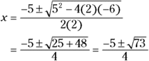
You have to solve the quadratic equation ![]() , for example, with the quadratic formula. Letting
, for example, with the quadratic formula. Letting ![]() ,
, ![]() , and
, and ![]() , you get
, you get
If you get a negative number under the radical when using the quadratic formula, you know that the problem has no real answer. Chapter 14 explains how to deal with these imaginary/complex answers.
Formulating huge quadratic results
Factoring a quadratic equation is almost always preferable to using the quadratic formula. But at certain times, you’re better off opting for the quadratic formula, even when you can factor the equation. In cases where the numbers are huge and have many multiplication possibilities, I suggest that you bite the bullet, haul out your calculator, and go for it.
For instance, a great problem in calculus (known as “Finding the largest box that can be formed from a rectangular piece of cardboard” for the curious among you) has an answer that you find when you solve the quadratic equation ![]() . The factors of 48 are 1, 2, 3, 4, 6, 8, 12, 16, 24, and 48. You can find that 125 has only four factors: 1, 5, 25, and 125. Using the method of multiplying
. The factors of 48 are 1, 2, 3, 4, 6, 8, 12, 16, 24, and 48. You can find that 125 has only four factors: 1, 5, 25, and 125. Using the method of multiplying ![]() times 125 and finding factors of
times 125 and finding factors of ![]() could take a lot of time and effort. Instead, using the quadratic formula and a handy-dandy calculator, you find the following:
could take a lot of time and effort. Instead, using the quadratic formula and a handy-dandy calculator, you find the following:
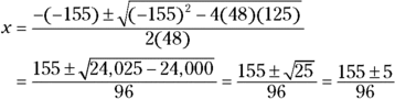
Starting with the plus sign, you get ![]() . For the minus sign, you get
. For the minus sign, you get ![]() . The fact that you get fractions tells you that you could’ve factored the quadratic:
. The fact that you get fractions tells you that you could’ve factored the quadratic: ![]() . Do you see where the 3 and 5 and the 16 and 25 come from in the answers?
. Do you see where the 3 and 5 and the 16 and 25 come from in the answers?
Completing the Square: Warming Up for Conics
Of all the choices you have for solving a quadratic equation (factoring and the quadratic formula, to name a couple; see the previous sections in this chapter), completing the square is usually your last resort. But the binomial-squared format is very nice to have when you’re working with conic sections (circles, ellipses, hyperbolas, and parabolas) and writing their standard forms (as you can see in Chapter 11).
For instance, using completing the square on the equation of a parabola gives you a visual answer to questions about where the vertex is and how it opens (to the side, up, or down; see Chapter 7). The big payoff is that you have a result for all your work. After all, you do get answers to the quadratic equations by using this process.
Squaring up a quadratic equation
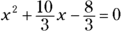
To solve a quadratic equation — such as ![]() — by completing the square, follow these steps:
— by completing the square, follow these steps:
Divide every term in the equation by the coefficient of the squared term.
For the example problem, you divide each term by the coefficient 3:
Move the constant term (the term without a variable) to the opposite side of the equation by adding or subtracting.
Add
 to each side:
 simplifies to
Find half the value of the coefficient on the first-degree term of the variable; square the result of the halving; and add that amount to each side of the equation.
Find half of
 , which is
  . Square the fraction, giving you
  and add the square to each side of the equation:
Factor the side of the equation that’s a perfect square trinomial (you just created it) into the square of a binomial.
Factor the left side of the equation:
 factors into
- Find the square root of each side of the equation.

Isolate the variable term by adding or subtracting to move the constant to the other side.
Subtract
 from each side and solve for the value of x:
The two answers are ![]() and
and ![]() .
.
You can verify the two example solutions by factoring the original equation: ![]() .
.
Completing the square twice over
Completing the square on an equation with both x’s and y’s leaves you just one step away from what you need to work with conics. Conic sections (circles, ellipses, hyperbolas, and parabolas) have standard equations that give you plenty of information about individual curves — where their centers are, which direction they go in, and so on. Chapter 11 covers this information in detail. In the meantime, you practice completing the square twice over in this section.
For example, you can write the equation ![]() as the sum of two binomials squared and a constant. Think of the equation as having two separate completing-the-square problems to, well, complete. Follow these steps to give the equation a twice-over:
as the sum of two binomials squared and a constant. Think of the equation as having two separate completing-the-square problems to, well, complete. Follow these steps to give the equation a twice-over:
- To handle the two completions more efficiently, rewrite the equation with a space between the x terms and the y terms and with the constant on the other side:
 You don’t divide through by the 2 on the
  term because that would leave you with a fractional coefficient on the
  term.
term. Find any numerical factors for each grouping — you want the coefficient of the squared term to be one. Write the factor outside parentheses with the variables inside.
In this case, you factor the 2 out of the two y terms and leave it outside the parentheses:

Complete the square on the x’s, and add whatever you used to complete the square to the other side of the equation, too, to keep the equation balanced.
Here, you take half of 6, square the 3 to get 9, and then add 9 to each side of the equation:

Complete the square on the y’s, and add whatever you used to complete the square to the other side of the equation, too.
If the trinomial is inside parentheses, be sure you multiply what you added by the factor outside the parentheses before adding to the other side.Completing the square on the y’s means you need to take half the value
 , square the
  to get
  , and then add 2(4) or 8 to each side:
Why do you add 8? Because when you put the 4 inside the parentheses with the y’s, you multiply by the 2. To keep the equation balanced, you put 4 inside the parentheses and 8 on the other side of the equation.
Simplify each side of the equation by writing the trinomials on the left as binomials squared and by combining the terms on the right.
For this example, you get
 .
.
You’re done — that is, until you get to Chapter 11, where you find out that you have an ellipse. How’s that for a cliffhanger?
Tackling Higher-Powered Polynomials
Solving polynomial equations requires that you know how to count and plan. Okay, so it isn’t really that simple. But if you can count up to the number that represents the degree (highest power) of the equation, you can account for the solutions you find and determine if you have them all. And if you can make a plan to use patterns in binomials or techniques from quadratics, you’re well on your way to a solution.
Handling the sum or difference of cubes
As I explain in Chapter 1, you factor an expression that’s the difference between two perfect squares into the difference and sum of the roots, ![]() . If you’re solving an equation that represents the difference of two squares, you can apply the multiplication property of zero and solve. However, you can’t factor the sum of two squares this way, so you’re usually out of luck when it comes to finding any real solution.
. If you’re solving an equation that represents the difference of two squares, you can apply the multiplication property of zero and solve. However, you can’t factor the sum of two squares this way, so you’re usually out of luck when it comes to finding any real solution.
In the earlier section “Factoring the difference of squares,” you see that something like ![]() has solutions
has solutions ![]() and
and ![]() . The equation
. The equation ![]() has no real solutions.
has no real solutions.
In the case of the difference or sum of two cubes, you can factor the binomial, and you do find a solution.
Here are the factorizations of the difference and sum of cubes:
Solving cubes by factoring
If you want to solve a cubic equation such as ![]() by using the factorization of the difference of cubes, you get
by using the factorization of the difference of cubes, you get ![]() . Using the multiplication property of zero (see Chapter 1), when
. Using the multiplication property of zero (see Chapter 1), when ![]() equals 0, x equals 4. But when
equals 0, x equals 4. But when ![]() , you need to use the quadratic formula, and you won’t be too happy with the results.
, you need to use the quadratic formula, and you won’t be too happy with the results.
Applying the quadratic formula, you get
You have a negative number under the radical, which means you find no real root. (Chapter 14 discusses what to do about negatives under radicals.) You deduce from this that the equation ![]() has just one real solution,
has just one real solution, ![]() .
.
Be careful when predicting the number of solutions of an equation from its power. In the previous example, the power three suggests that you may find as many as three solutions. But in actuality, the exponent just tells you that you can find no more than three solutions.
Solving cubes by taking the cube root
You may wonder if the factorization of the difference or sum of two perfect cubes always results in a quadratic factor that has no real roots (like the example I show in the preceding section, “Solving cubes by factoring”). Well, wonder no longer. The answer is a resounding “Yes!” When you factor a difference — ![]() — the quadratic
— the quadratic ![]() doesn’t have a real root; when you factor a sum —
doesn’t have a real root; when you factor a sum — ![]() — the equation
— the equation ![]() doesn’t have a real root, either.
doesn’t have a real root, either.
You can make the best of the fact that you find only one real root for equations in the cubic form by deciding how to deal with solving equations of that form. I suggest changing the equations ![]() and
and ![]() to
to ![]() and
and ![]() , respectively, and taking the cube root of each side.
, respectively, and taking the cube root of each side.
To solve ![]() , for example, rewrite it as
, for example, rewrite it as ![]() and then find the cube root,
and then find the cube root, ![]() . With the equation
. With the equation ![]() , you first subtract 125 from each side and then divide each side by 8 to get
, you first subtract 125 from each side and then divide each side by 8 to get ![]() .
.
When you take the cube root of a negative number, you get a negative root. A cube root is an odd root, so you can find cube roots of negatives. You can’t do roots of negative numbers if the roots are even (square root, fourth root, and so on). For the previous example, you find ![]() .
.
Tackling quadratic-like trinomials
A quadratic-like trinomial is a trinomial of the form ![]() . The power on one variable term is twice that of the other variable term, and a constant term completes the picture. The good thing about quadratic-like trinomials is that they’re candidates for factoring and then for the application of the multiplication property of zero (see Chapter 1). One such trinomial is
. The power on one variable term is twice that of the other variable term, and a constant term completes the picture. The good thing about quadratic-like trinomials is that they’re candidates for factoring and then for the application of the multiplication property of zero (see Chapter 1). One such trinomial is ![]() .
.
You can think of this equation as being like the quadratic ![]() , which factors into
, which factors into ![]() . If you replace the x’s in the factorization with
. If you replace the x’s in the factorization with ![]() , you have the factorization for the equation with the z’s.
, you have the factorization for the equation with the z’s.
Then you then set each factor equal to zero. When ![]() ,
, ![]() , and
, and ![]() . And when
. And when ![]() ,
, ![]() , and
, and ![]() .
.
You can just take the cube roots of each side of the equations you form (see the previous section), because when you take that odd root, you know you can find only one real solution.
Here’s another example. When solving the quadratic-like trinomial ![]()
![]() , you can factor the left side and then factor the factors again:
, you can factor the left side and then factor the factors again: ![]() .
.
Setting the individual factors equal to zero, you get ![]() ,
, ![]() ,
, ![]() ,
, ![]() .
.
Solving Quadratic Inequalities
A quadratic inequality is just what it says: an inequality (![]() ,
, ![]() ,
, ![]() , or
, or ![]() ) that involves a quadratic expression. You can employ the same method you use when solving a quadratic inequality to solve high-degree inequalities and rational inequalities (which contain variables in fractions).
) that involves a quadratic expression. You can employ the same method you use when solving a quadratic inequality to solve high-degree inequalities and rational inequalities (which contain variables in fractions).
You need to be able to solve quadratic equations in order to solve quadratic inequalities. With quadratic equations, you set the expressions equal to zero; inequalities deal with what’s on either side of the zero (positives and negatives).
To solve a quadratic inequality, follow these steps:
- Move all the terms to one side of the inequality sign.
- Factor, if possible.
Determine all zeros (roots, or solutions).
Zeros are the values of the variable that make each factored expression equal to zero. (Check out the “The name game: Solutions, roots, and zeros” sidebar in this chapter for information on these terms.)
- Put the zeros in order on a number line.
Create a sign-line to show where the expression in the inequality is positive or negative.
A sign-line shows the signs of the different factors in each interval. If the expression is factored, show the signs of the individual factors.
- Determine the solution, writing it in inequality notation or interval notation (I cover interval notation in Chapter 1).
Keeping inequality strictly quadratic
The techniques you use to solve the inequalities in this section are also applicable for solving higher degree polynomial inequalities and rational inequalities. If you can factor a third- or fourth-degree polynomial (see the previous section to get started), you can handily solve an inequality where the polynomial is set less than zero or greater than zero. You can also use the sign-line method to look at factors of rational (fractional) expressions. For now, however, consider sticking to the quadratic inequalities.
To solve the inequality ![]() , for example, you need to determine what values of x you can square so that when you subtract the original number, your answer will be bigger than 12. For instance, when
, for example, you need to determine what values of x you can square so that when you subtract the original number, your answer will be bigger than 12. For instance, when ![]() , you get
, you get ![]() . That’s certainly bigger than 12, so the number 5 works;
. That’s certainly bigger than 12, so the number 5 works; ![]() is a solution. How about the number 2? When
is a solution. How about the number 2? When ![]() , you get
, you get ![]() , which isn’t bigger than 12. You can’t use
, which isn’t bigger than 12. You can’t use ![]() in the solution. Do you then conclude that smaller numbers don’t work? Not so. When you try
in the solution. Do you then conclude that smaller numbers don’t work? Not so. When you try ![]() , you get
, you get ![]() , which is most definitely bigger than 12. You can actually find an infinite amount of numbers that make this inequality a true statement. Rather than keep guessing the answers, the following gives you a procedure.
, which is most definitely bigger than 12. You can actually find an infinite amount of numbers that make this inequality a true statement. Rather than keep guessing the answers, the following gives you a procedure.
Solve the quadratic inequality by using the steps I outline in the introduction to this section:
Subtract 12 from each side of the inequality
 to move all the terms to one side.
You end up with
 .
.- Factoring on the left side of the inequality, you get
 .
. - Determine that all the zeros for the inequality are
 and
and  .
. - Put the zeros in order on a number line, shown in the following figure.

Create a sign-line to show the signs of the different factors in each interval.
Between –3 and 4, try letting
 (you can use any number between
  and 4). When
  , the factor
  is negative, and the factor
  is positive. Put those signs on the sign-line to correspond to the factors. Do the same for the interval of numbers to the left of –3 and to the right of 4 (see the following illustration).
 The x-values in each interval are really random choices (as you can see from my choice of
  and
and  ). Any number in each of the intervals gives you the same positive or negative value to the factor.
To determine the solution, look at the signs of the factors; you want the expression to be positive, corresponding to the inequality greater than zero.
The interval to the left of
 has a negative times a negative, which is positive. So, any number to the left of
  works. You can write that part of the solution as
  or, in interval notation (see Chapter 1),
  . The interval to the right of 4 has a positive times a positive, which is positive. So,
  is a solution; you can write it as
  . The interval between
  and 4 is always negative; you have a negative times a positive. The complete solution lists both intervals that have working values in the inequality.
The solution of the inequality
 , therefore, is
  or
or  . Writing this result in interval notation, you replace the word “or” with the symbol
  and write it as
  .
.
Signing up for fractions
The sign-line process (see the introduction to this section and the previous example problem) is great for solving rational inequalities, such as ![]() .
.
The signs of the results of multiplication and division use the same rules, so to determine your answer, you can treat the numerator and denominator the same way you treat two different factors in multiplication.
Using the steps from the list I present in the introduction to this section, determine the solution for a rational inequality:
- Every term in
 is to the left of the inequality sign.
 - Neither the numerator nor the denominator factors any further.
- The two zeros are
 and
and  .
. - You can see the two numbers on a number line in the following illustration.

- Create a sign-line for the two zeros; you can see in the following figure that the numerator is positive when x is greater than 2, and the denominator is positive when x is greater than
 .
.

When determining the solution, keep in mind that the inequality calls for something less than or equal to zero.
The fraction is a negative number when you choose an x between
 and 2. You get a negative numerator and a positive denominator, which gives a negative result. Another solution to the original inequality is the number 2. Letting
  , you get a numerator equal to 0, which you want because the inequality is less than or equal to zero. You can’t let the denominator be zero, though. Having a zero in the denominator isn’t allowed because no such number exists. So, the solution of
 . In interval notation, you write the solution as
  . (For more on interval notation, see Chapter 2.)
Increasing the number of factors
The method you use to solve a quadratic inequality (see the section “Keeping inequality strictly quadratic”) works nicely with fractions and higher-degree expressions. For example, you can solve ![]() by creating a sign-line and checking the products.
by creating a sign-line and checking the products.
The inequality is already factored, so you move to the step (Step 3) where you determine the zeros. The zeros are ![]() and 5 (the 5 is a double root and the factor is always positive or 0). The following illustration shows the values in order on the number line.
and 5 (the 5 is a double root and the factor is always positive or 0). The following illustration shows the values in order on the number line.

Now you choose a number in each interval, substitute the numbers into the expression on the left of the inequality, and determine the signs of the four factors in those intervals. You can see from the following figure that the last factor, ![]() , is always positive or zero, so that’s an easy factor to pinpoint.
, is always positive or zero, so that’s an easy factor to pinpoint.

You want the expression on the left to be positive or zero, given the original language of the inequality. You find an even number of negative factors between ![]() and
and ![]() and for numbers greater than 4 (zero is an even number). You include the zeros, so the solution you find is
and for numbers greater than 4 (zero is an even number). You include the zeros, so the solution you find is ![]() or
or ![]() . In interval notation, you write the solution as
. In interval notation, you write the solution as ![]() . (For more on interval notation, see Chapter 2.)
. (For more on interval notation, see Chapter 2.)
Considering absolute value inequalities
Another type of inequality that you can solve using this sign-line method is an absolute value inequality involving a quadratic or higher-degree variable. The process is pretty much the same as with quadratic or polynomial inequalities. The only difference comes in the evaluation of the intervals — you refer to the original statement.
For example, to solve ![]() , you first factor the cubic to get
, you first factor the cubic to get ![]() . The three zeros are
. The three zeros are ![]() ,
, ![]() , and
, and ![]() . Put them on a sign line and establish the signs of the intervals determined. This part is really quite simple to evaluate; the expression is always positive (except at the zeros). The absolute value operation creates all positive or 0 results. So the solution is
. Put them on a sign line and establish the signs of the intervals determined. This part is really quite simple to evaluate; the expression is always positive (except at the zeros). The absolute value operation creates all positive or 0 results. So the solution is ![]() or
or ![]() or
or ![]() or
or ![]() . An easier way to read the solution is to just say the solution is all real numbers except for
. An easier way to read the solution is to just say the solution is all real numbers except for ![]() ,
, ![]() , or
, or ![]() . Or there’s the interval notation:
. Or there’s the interval notation: ![]() .
.