Chapter 7
Sketching and Interpreting Quadratic Functions
IN THIS CHAPTER
![]() Mastering the standard form of quadratics
Mastering the standard form of quadratics
![]() Locating the x- and y-intercepts
Locating the x- and y-intercepts
![]() Reaching the extremes of quadratics
Reaching the extremes of quadratics
![]() Putting the axis of symmetry into play
Putting the axis of symmetry into play
![]() Piecing together all kinds of quadratic puzzles
Piecing together all kinds of quadratic puzzles
![]() Watching quadratics at work in the real world
Watching quadratics at work in the real world
Aquadratic function is one of the more recognizable and useful polynomial (multi-termed) functions found in all of algebra. The function describes a graceful U-shaped curve called a parabola that you can quickly sketch and easily interpret. People use quadratic functions to model economic situations, physical training progress, and the paths of comets. How much more useful can math get?
The most important features to recognize in order to sketch a parabola are the opening (up or down, steep or wide), the intercepts, the vertex, and the axis of symmetry. In this chapter, I show you how to identify all these features within the standard form of the quadratic function. I also show you some equations of parabolas that model events.
Interpreting the Standard Form of Quadratics
A parabola is the graph of a quadratic function. The graph is a nice, gentle, U-shaped curve that has points located an equal distance on either side of a line running up through its middle — called its axis of symmetry. Parabolas can be turned upward, downward, left, or right, but parabolas that represent functions only turn up or down. (In Chapter 11, you find out more about the other types of parabolas in the general discussion of conics.) The standard form for the quadratic function is
The coefficients (multipliers of the variables) a, b, and c are real numbers; the coefficient a can’t be equal to zero because you’d no longer have a quadratic function. You have plenty to discover from the simple standard form equation. The coefficients a and b are important, and some equations may not have all three of the terms in them. As you can see, there’s meaning in everything (or nothing)!
Starting with “a” in the standard form
As the lead coefficient of the standard form of the quadratic function ![]() , a gives you two bits of information: the direction in which the graphed parabola opens, and whether the parabola is steep or flat. Here’s the breakdown of how the sign and size of the lead coefficient, a, affect the parabola’s appearance:
, a gives you two bits of information: the direction in which the graphed parabola opens, and whether the parabola is steep or flat. Here’s the breakdown of how the sign and size of the lead coefficient, a, affect the parabola’s appearance:
- If a is positive, the graph of the parabola opens upward (see Figures 7-1a and 7-1b).
- If a is negative, the graph of the parabola opens downward (see Figures 7-1c and 7-1d).
- If a has an absolute value greater than one, the graph of the parabola is steep (see Figures 7-1a and 7-1c). (See Chapter 2 for a refresher on absolute values.)
- If a has an absolute value less than one, the graph of the parabola flattens out (see Figures 7-1b and 7-1d).

John Wiley & Sons, Inc.
FIGURE 7-1: Parabolas opening up and down, appearing steep and flat.
 If you remember the four rules that identify the lead coefficient of a parabola, you don’t even have to graph the equation to describe how the parabola looks. Here’s how you can describe some parabolas from their equations:
 : You say that this parabola is steep and opens upward because the lead coefficient is positive and greater than one.
 : You say that this parabola is flattened out and opens downward because the lead coefficient is negative, and the absolute value of the fraction is less than one.
 : You say that this parabola is flattened out and opens upward because the lead coefficient is positive, and the decimal value is less than one. In fact, the coefficient is so small that the flattened parabola almost looks like a horizontal line.
Following up with “b” and “c”
Much like the lead coefficient in the quadratic function (see the previous section), the values of b and c give you plenty of information. Mainly, the values tell you a lot if they’re not there. In the next section, you find out how to use these values to find intercepts (or zeros). For now, you concentrate on their presence or absence.
The lead coefficient, a, can never be equal to zero. If that happens, you no longer have a quadratic function, and this discussion is finished. As for the other two terms:
- If the second coefficient, b, is zero, the parabola straddles the y-axis. The parabola’s vertex — the highest or lowest point on the curve, depending on which way it faces — is on that axis, and the parabola is symmetric about the axis (see Figure 7-2a, a graph of a quadratic function where
 ). The second term in the standard form is the x term, so if the coefficient b is zero, the second term disappears. The standard equation becomes
  , which makes finding intercepts very easy (see the following section).
 - If the last term, c, is zero, the graph of the parabola goes through the origin — in other words, one of its intercepts is the origin (see Figure 7-2b, a graph of a quadratic function where
 ). The standard equation becomes
  , which you can easily factor into
  . (See Chapters 1 and 3 for more on factoring.)

John Wiley & Sons, Inc.
FIGURE 7-2: Graphs of  and
and  .
.
Investigating Intercepts in Quadratics
The intercepts of a quadratic function (or any function) are the points where the graph of the function crosses the x-axis or y-axis. The graph of a function can cross the x-axis any number of times, but it can cross the y-axis only once.
Why be concerned about the intercepts of a parabola? In real-life situations, the intercepts occur at points of interest — for instance, at the initial value of an investment or at the break-even point for a business.
Intercepts are also very helpful when you’re graphing a parabola. The points are easy to find because one of the coordinates is always zero. If you have the intercepts, the vertex (see “Going to the Extreme: Finding the Vertex” later in the chapter), and what you know about the symmetry of the parabola (as I discuss in the section “Lining Up along the Axis of Symmetry”), you have a good idea of what the graph looks like.
Finding the one and only y-intercept
The y-intercept of a quadratic function is ![]() . A parabola with the standard equation
. A parabola with the standard equation ![]() is a function, so by definition (as I cover in Chapter 6), only one y value can exist for every x value. When
is a function, so by definition (as I cover in Chapter 6), only one y value can exist for every x value. When ![]() , as it does at the y-intercept, the equation becomes
, as it does at the y-intercept, the equation becomes ![]() , or
, or ![]() . The statements
. The statements ![]() and
and ![]() combine to become the y-intercept,
combine to become the y-intercept, ![]() .
.
To find the y-intercepts of the following functions, you let ![]() :
:
 : When
  ,
,  (or
(or  ). The y-intercept is (0, 2).
 : When
  ,
,  (or
(or  ); don’t let the missing x term throw you. The y-intercept is
  .
. : When
  ,
,  . The equation provides no constant term; you could also say the missing constant term is zero. The y-intercept is (0, 0).
People can model many situations with quadratic functions, and the places where the input variables or output variables equal zero are important. For example, a candle-making company has figured out that its profit is based on the number of candles it produces and sells. The company uses the function ![]() — where x represents the number of candles — to determine P, the profit. As you can see from the equation, the graph of this parabola opens downward (because a is negative; see the section “Starting with ‘a’ in the standard form”). Figure 7-3 is a sketch of the graph of the profit, with the y-axis representing profit and the x-axis representing the number of candles.
— where x represents the number of candles — to determine P, the profit. As you can see from the equation, the graph of this parabola opens downward (because a is negative; see the section “Starting with ‘a’ in the standard form”). Figure 7-3 is a sketch of the graph of the profit, with the y-axis representing profit and the x-axis representing the number of candles.

John Wiley & Sons, Inc.
FIGURE 7-3: A company can determine its profit with a quadratic equation.
Does it make sense to use a quadratic function to model profit? Why would the profit decrease after a certain point? Does that make business sense? It does if you consider that perhaps, when you make too many candles, the cost of overtime and the need for additional machinery play a part.
What about the y-intercept? What part does it play, and what does it mean in this candle-making case? You can say that ![]() represents not producing or selling any candles. According to the equation and graph, the y-intercept has a y-coordinate of
represents not producing or selling any candles. According to the equation and graph, the y-intercept has a y-coordinate of ![]() . It makes sense to find a negative profit if the company has costs that it has to pay no matter what (even if it sells no candles): insurance, salaries, mortgage payments, and so on. With some interpretation, you can find a logical explanation for the y-intercept being negative in this case.
. It makes sense to find a negative profit if the company has costs that it has to pay no matter what (even if it sells no candles): insurance, salaries, mortgage payments, and so on. With some interpretation, you can find a logical explanation for the y-intercept being negative in this case.
Finding the x-intercepts
You find the x-intercepts of quadratics when you solve for the zeros, or solutions, of the quadratic equation. The method you use to solve for the zeros is the same method you use to solve for the intercepts, because they’re really just the same thing. The names change (intercept, zero, solution), depending on the application, but you find the intercepts the same way.
Parabolas with an equation of the standard form ![]() open upward or downward and may or may not have x-intercepts. Look at Figure 7-4, for example. You see a parabola with two x-intercepts (Figure 7-4a), one with a single x-intercept (Figure 7-4b), and one with no x-intercept (Figure 7-4c). Notice, however, that they all have a y-intercept.
open upward or downward and may or may not have x-intercepts. Look at Figure 7-4, for example. You see a parabola with two x-intercepts (Figure 7-4a), one with a single x-intercept (Figure 7-4b), and one with no x-intercept (Figure 7-4c). Notice, however, that they all have a y-intercept.

John Wiley & Sons, Inc.
FIGURE 7-4: Parabolas can intercept the x-axis multiple times, a single time, or not at all.
The coordinates of all x-intercepts have zeros in them. An x-intercept’s y value is zero, and you write it in the form (h, 0). How do you find the value of h? You let ![]() in the general equation and then solve for x. You have two options when solving the equation
in the general equation and then solve for x. You have two options when solving the equation ![]() :
:
- Use the quadratic formula (refer to Chapter 3 for a refresher on the formula).
- Try to factor the expression and use the multiplication property of zero (you can find more on this in Chapter 1).
Regardless of the path you take, you have some guidelines at your disposal to help you determine the number of x-intercepts you should find.
When finding x-intercepts by solving ![]() ,
,
- You find two x-intercepts if
- The expression factors into two different binomials.
- The quadratic formula gives you a value greater than zero under the radical.
- You find one x-intercept (a double root) if
- The expression factors into the square of a binomial.
- The quadratic formula gives you a value of zero under the radical.
- You find no x-intercept if both
- The expression doesn’t factor.
- The quadratic formula gives you a value less than zero under the radical (indicating an imaginary root; Chapter 14 deals with imaginary and complex numbers).
To find the x-intercepts of ![]() , for example, you can set y equal to zero and solve the quadratic equation by factoring:
, for example, you can set y equal to zero and solve the quadratic equation by factoring:

- When
 ,
,  ; and when
  ,
,  .
.
The two intercepts are ![]() and
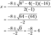
and ![]() ; you can see that the equation factors into two different factors. In cases where you can’t figure out how to factor the quadratic, you can get the same answer by using the quadratic formula. I show you how to do this, using the quadratic that I just factored. Notice in the following calculation that the value under the radical is a number greater than zero, meaning that you have two answers:
; you can see that the equation factors into two different factors. In cases where you can’t figure out how to factor the quadratic, you can get the same answer by using the quadratic formula. I show you how to do this, using the quadratic that I just factored. Notice in the following calculation that the value under the radical is a number greater than zero, meaning that you have two answers:

When performing the addition in the numerator, you have ![]() . And when performing the subtraction,
. And when performing the subtraction, ![]() . The answers are, of course, the same.
. The answers are, of course, the same.
Here’s another example, with a different result. To find the x-intercepts of ![]() , you can set y equal to zero and solve the quadratic equation by factoring:
, you can set y equal to zero and solve the quadratic equation by factoring:

- So when
 ,
,  .
.
The only intercept is (4, 0). The equation factors into the square of a binomial — a double root. You can get the same answer by using the quadratic formula — notice that the value under the radical is equal to zero:
This last example shows how you determine that an equation has no x-intercept. To find the x-intercepts of ![]() , you can set y equal to zero and try to factor the quadratic equation, but you can’t do it. The equation has no factors that give you this quadratic.
, you can set y equal to zero and try to factor the quadratic equation, but you can’t do it. The equation has no factors that give you this quadratic.
When you try the quadratic formula, you see that the value under the radical is less than zero; a negative number under the radical is an imaginary number:
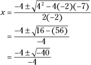
Alas, you find no x-intercept for this parabola.
Going to the Extreme: Finding the Vertex
Quadratic functions, or parabolas, that have the standard form ![]() are gentle, U-shaped curves that open either upward or downward. When the lead coefficient, a, is a positive number, the parabola opens upward, creating a minimum value for the function — the function values never go lower than that minimum. When a is negative, the parabola opens downward, creating a maximum value for the function — the function values never go higher than that maximum.
are gentle, U-shaped curves that open either upward or downward. When the lead coefficient, a, is a positive number, the parabola opens upward, creating a minimum value for the function — the function values never go lower than that minimum. When a is negative, the parabola opens downward, creating a maximum value for the function — the function values never go higher than that maximum.
 The two extreme values, the minimum and maximum, occur at the parabola’s vertex. The y-coordinate of the vertex gives you the numerical value of the extreme — its highest or lowest point.
The vertex of a parabola is very useful for finding the extreme value, so certainly algebra provides an efficient way of finding it. Right? Well, sure it does! The vertex serves as a sort of anchor for the two parts of the curve to flare out from. The axis of symmetry (see the following section) runs through the vertex. The y-coordinate of the vertex is the function’s maximum or minimum value — again, depending on which way the parabola opens.
 The parabola
 ![]() has its vertex where
has its vertex where ![]() . You plug in the a and b values from the equation to come up with x, and then you find the y-coordinate of the vertex by plugging this x value into the equation and solving for y.
. You plug in the a and b values from the equation to come up with x, and then you find the y-coordinate of the vertex by plugging this x value into the equation and solving for y.
To find the coordinates of the vertex of the equation ![]() , for example, you substitute the coefficients a and b into the equation for x:
, for example, you substitute the coefficients a and b into the equation for x:
You solve for y by putting the x value back into the equation:
The coordinates of the vertex are (2, 5). You find a maximum value, because a is a negative number, which means the parabola opens downward from this point. The graph of the parabola never goes higher than five units above the x-axis.
 When an equation leaves out the b value, make sure you don’t substitute the c value for the b value in the vertex equation. For example, to find the coordinates of the vertex of
 ![]() , you substitute the coefficients a (4) and b (0) into the equation for x:
, you substitute the coefficients a (4) and b (0) into the equation for x:
You solve for y by putting the x value into the equation:
The coordinates of the vertex are ![]() . You have a minimum value, because a is a positive number, meaning the parabola opens upward from the minimum point.
. You have a minimum value, because a is a positive number, meaning the parabola opens upward from the minimum point.
Lining Up along the Axis of Symmetry
The axis of symmetry of a quadratic function is a vertical line that runs through the vertex of the parabola (see the previous section) and acts as a mirror — half the parabola rests on one side of the axis, and half rests on the other. The x-value in the coordinates of the vertex appears in the equation for the axis of symmetry. For instance, if a vertex has the coordinates (2, 3), the axis of symmetry is ![]() . All vertical lines have an equation of the form
. All vertical lines have an equation of the form ![]() . In the case of the axis of symmetry, the h is always the x-coordinate of the vertex.
. In the case of the axis of symmetry, the h is always the x-coordinate of the vertex.
The axis of symmetry is useful because when you’re sketching a parabola and finding the coordinates of a point that lies on it, you know you can find another point that exists as a partner to your point, in that
- It lies on the same horizontal line.
- It lies on the other side of the axis of symmetry.
- It covers the same distance from the axis of symmetry as your point.
Maybe I should just show you what I mean with a sketch! Figure 7-5 shows points on a parabola that lie on the same horizontal line and on either side of the axis of symmetry.

John Wiley & Sons, Inc.
FIGURE 7-5: Points resting on the same horizontal line and equidistant from the axis of symmetry.
The points ![]() and
and ![]() are each two units from the axis — the line
are each two units from the axis — the line ![]() . The points
. The points ![]() and (6, 7) are each four units from the axis. And the points
and (6, 7) are each four units from the axis. And the points ![]() and (5, 0), the x-intercepts, are each three units from the axis.
and (5, 0), the x-intercepts, are each three units from the axis.
Sketching a Graph from the Available Information
You have all sorts of information available when it comes to a parabola and its graph. You can use the intercepts, the opening, the steepness, the vertex, the axis of symmetry, or just some random points to plot the parabola; you don’t really need all the pieces. As you practice sketching these curves, it becomes easier to figure out which pieces you need for different situations. Sometimes the x-intercepts are hard to find, so you concentrate on the vertex, direction, and axis of symmetry. Other times you find it more convenient to use the y-intercept, a point or two on the parabola, and the axis of symmetry. This section provides you with a couple examples. Of course, you can go ahead and check off all the information that’s possible. Some people are very thorough that way.
To sketch the graph of ![]() , first notice that the equation represents a parabola that opens upward (see the section “Starting with ‘a’ in the standard form”), because the lead coefficient, a, is positive
, first notice that the equation represents a parabola that opens upward (see the section “Starting with ‘a’ in the standard form”), because the lead coefficient, a, is positive ![]() . The y-intercept is (0, 1), which you get by plugging in zero for x. If you set y equal to zero to solve for the x-intercepts, you get
. The y-intercept is (0, 1), which you get by plugging in zero for x. If you set y equal to zero to solve for the x-intercepts, you get ![]() , which doesn’t factor. You could whip out the quadratic formula — but wait. You have other possibilities to consider.
, which doesn’t factor. You could whip out the quadratic formula — but wait. You have other possibilities to consider.
The vertex is more helpful than finding the intercepts in this case because of its convenience — you don’t have to work so hard to get the coordinates. Use the formula for the x-coordinate of the vertex to get ![]() (see the section “Going to the Extreme: Finding the Vertex”). Plug the 4 into the formula for the parabola, and you find that the vertex is at (4, –15). This coordinate is below the x-axis, and the parabola opens upward, so the parabola does have x-intercepts; you just can’t find them easily because they’re irrational numbers (square roots of numbers that aren’t perfect squares).
(see the section “Going to the Extreme: Finding the Vertex”). Plug the 4 into the formula for the parabola, and you find that the vertex is at (4, –15). This coordinate is below the x-axis, and the parabola opens upward, so the parabola does have x-intercepts; you just can’t find them easily because they’re irrational numbers (square roots of numbers that aren’t perfect squares).
You can try whipping out your graphing calculator to get some decimal approximations of the intercepts (see Chapter 5 for info on using a graphing calculator). Or, instead, you can find a point and its partner point on the other side of the axis of symmetry, which is ![]() (see the section “Lining Up along the Axis of Symmetry”). If you let
(see the section “Lining Up along the Axis of Symmetry”). If you let ![]() , for example, you find that
, for example, you find that ![]() . This point is three units from
. This point is three units from ![]() , to the left; you find the distance by subtracting
, to the left; you find the distance by subtracting ![]() . Use this distance to find three units to the right,
. Use this distance to find three units to the right, ![]() . The corresponding point is
. The corresponding point is ![]() .
.
If you sketch all that information in a graph first — the y-intercept, vertex, axis of symmetry, and the points ![]() and
and ![]() — you can identify the shape of the parabola and sketch in the whole thing. Figure 7-6 shows the two steps: putting in the information (Figure 7-6a), and sketching in the parabola (Figure 7-6b).
— you can identify the shape of the parabola and sketch in the whole thing. Figure 7-6 shows the two steps: putting in the information (Figure 7-6a), and sketching in the parabola (Figure 7-6b).

John Wiley & Sons, Inc.
FIGURE 7-6: Using the various pieces of a quadratic as steps for sketching a parabola.
Here’s another example for practice. To sketch the graph of ![]() , look for the hints. The parabola opens downward (because a is negative) and is pretty flattened out (because the absolute value of a is less than zero). The graph goes through the origin because the constant term (c) is missing. Therefore, the y-intercept and one of the x-intercepts is (0, 0). The vertex lies at
, look for the hints. The parabola opens downward (because a is negative) and is pretty flattened out (because the absolute value of a is less than zero). The graph goes through the origin because the constant term (c) is missing. Therefore, the y-intercept and one of the x-intercepts is (0, 0). The vertex lies at ![]() . To solve for the other x-intercept, let
. To solve for the other x-intercept, let ![]() and factor:
and factor:
The second factor tells you that the other x-intercept occurs when ![]() . The intercepts and vertex are sketched in Figure 7-7a.
. The intercepts and vertex are sketched in Figure 7-7a.

John Wiley & Sons, Inc.
FIGURE 7-7: Using intercepts and the vertex to sketch a parabola.
You can add the point ![]() for a little more help with the shape of the parabola by using the axis of symmetry (see the section “Lining Up along the Axis of Symmetry”). See how you can draw the curve in? Figure 7-7b shows you the way. It really doesn’t take much to do a decent sketch of a parabola.
for a little more help with the shape of the parabola by using the axis of symmetry (see the section “Lining Up along the Axis of Symmetry”). See how you can draw the curve in? Figure 7-7b shows you the way. It really doesn’t take much to do a decent sketch of a parabola.
Applying Quadratics to the Real World
Quadratic functions are wonderful models for many situations that occur in the real world. You can see them at work in financial and physical applications, just to name a couple. This section provides a few applications for you to consider.
Selling candles
A candle-making company has figured out that its profit is based on the number of candles it produces and sells. The function ![]() applies to the company’s situation, where x represents the number of candles, and P represents the profit. You may recognize this function from the section “Investigating Intercepts in Quadratics” earlier in the chapter. You can use the function to find out how many candles the company has to produce to garner the greatest possible profit.
applies to the company’s situation, where x represents the number of candles, and P represents the profit. You may recognize this function from the section “Investigating Intercepts in Quadratics” earlier in the chapter. You can use the function to find out how many candles the company has to produce to garner the greatest possible profit.
You find the two x-intercepts by letting y = 0 and solving for x by factoring:

- When
 , you have
  ; and when
  ,
,  . These two numbers give you the two x-intercepts: (20, 0) and (140, 0).
The intercept (20, 0) represents where the function (the profit) changes from negative values to positive values. You know this because the graph of the profit function is a parabola that opens downward (because a is negative), so the beginning and ending of the curve appear below the x-axis. The intercept (140, 0) represents where the profit changes from positive values to negative values. So, the maximum value, the vertex, lies somewhere between and above the two intercepts (see the section “Going to the Extreme: Finding the Vertex”). The x-coordinate of the vertex lies between 20 and 140. Refer to Figure 7-3 if you want to see the graph again.
You now use the formula for the x-coordinate of the vertex to find ![]() . The number 80 lies between 20 and 140; in fact, it rests halfway between them. The nice, even number is due to the symmetry of the graph of the parabola and the symmetric nature of these functions. Now you can find the P value (the y-coordinate of the vertex):
. The number 80 lies between 20 and 140; in fact, it rests halfway between them. The nice, even number is due to the symmetry of the graph of the parabola and the symmetric nature of these functions. Now you can find the P value (the y-coordinate of the vertex): ![]()
![]() .
.
Your findings say that if the company produces and sells 80 candles, the maximum profit will be $180. That seems like an awful lot of work for $180, but maybe the company runs a small business. Work such as this shows you how important it is to have models for profit, revenue, and cost in business so you can make projections and adjust your plans.
Shooting basketballs
A local youth group recently raised money for charity by having a Throw-A-Thon. Participants prompted sponsors to donate money based on a promise to shoot baskets over a 12-hour period. This was a very successful project, both for charity and for algebra, because you can find some interesting bits of information about shooting the basketballs and the number of misses that occurred.
Participants shot baskets for 12 hours, attempting about 200 baskets each hour. The quadratic equation ![]() models the number of baskets they missed each hour, where t is the time in hours (numbered from 0 through 12) and M is the number of misses.
models the number of baskets they missed each hour, where t is the time in hours (numbered from 0 through 12) and M is the number of misses.
This quadratic function opens upward (because a is positive), so the function has a minimum value. Figure 7-8 shows a graph of the function.

John Wiley & Sons, Inc.
FIGURE 7-8: The downs and ups of shooting baskets.
From the graph, you see that the initial value, the y-intercept, is 100. At the beginning, participants were missing about 100 baskets per hour. The good news is that they got better with practice. ![]() , which means that at hour two into the project, the participants were missing only 60 baskets per hour. The number of misses goes down and then goes back up again. How do you interpret this? Even though the participants got better with practice, they let the fatigue factor take over.
, which means that at hour two into the project, the participants were missing only 60 baskets per hour. The number of misses goes down and then goes back up again. How do you interpret this? Even though the participants got better with practice, they let the fatigue factor take over.
What’s the fewest number of misses per hour? When did the participants shoot their best? To answer these questions, find the vertex of the parabola by using the formula for the x-coordinate (you can find this in the “Going to the Extreme: Finding the Vertex” section earlier in the chapter):
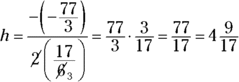
The best shooting happened about 4.5 hours into the project. How many misses occurred then? The number you get represents what’s happening the entire hour — although that’s fudging a bit:
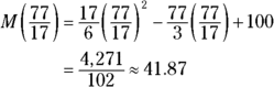
The fraction is rounded to two decimal places. The best shooting is about 42 misses that hour.
Launching a water balloon
One of the favorite springtime activities of the engineering students at a certain university is to launch water balloons from the top of the engineering building so they hit the statue of the school’s founder, which stands 25 feet from the building. The launcher sends the balloons up in an arc to clear a tree that sits next to the building. To hit the statue, the initial velocity and angle of the balloon have to be just right. Figure 7-9 shows a successful launch.

John Wiley & Sons, Inc.
FIGURE 7-9: Launching a water balloon over a tree requires more math than you think.
This year’s launch was successful. The students found that by launching the water balloons at 48 feet per second with a precise angle, they could hit the statue. Here’s the equation they worked out to represent the path of the balloons: ![]() . The t represents the number of seconds, and H is the height of the balloon in feet. From this quadratic function, you can answer the following questions:
. The t represents the number of seconds, and H is the height of the balloon in feet. From this quadratic function, you can answer the following questions:
How high is the building?
Solving the first question is probably easy for you. The launch occurs at time
 , the initial value of the function. When
  ,
, 
 . The building is 60 feet high.
How high did the balloon travel?
You answer the second question by finding the vertex of the parabola:
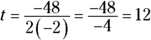 . This gives you t, the number of seconds it takes the balloon to get to its highest point — 12 seconds after launch. Substitute the answer into the equation to get the height:
  . The balloon went 348 feet into the air.
If the statue is 10 feet tall, how many seconds did it take for the balloon to reach the statue after the launch?
To solve the third question, use the fact that the statue is 10 feet high; you want to know when
 . Replace H with 10 in the equation and solve for t by factoring (see Chapters 1 and 3):
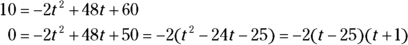
When
 ,
,  . And when
  ,
,  .
.According to the equation, the amount of time is either 25 seconds or
 second. The
  doesn’t really make any sense because you can’t go back in time; if the balloon had started at the ground level, it would have taken that one second to reach that initial 60 feet in the air. The 25 seconds, however, tells you how long it took the balloon to reach the statue. Imagine the anticipation!