Chapter 6
Formulating Function Facts
IN THIS CHAPTER
![]() Freeze-framing function characteristics
Freeze-framing function characteristics
![]() Concentrating on domain and range
Concentrating on domain and range
![]() Tackling one-to-one functions
Tackling one-to-one functions
![]() Joining the “piece” corps
Joining the “piece” corps
![]() Handling composition duties
Handling composition duties
![]() Working with inverses
Working with inverses
Is your computer functioning well? Are you going to that company function? Are his kidneys functioning properly? What is all this business about functions? In algebra, the word function is very specific. You reserve it for certain math expressions that meet the tough standards of input and output values, as well as other mathematical rules of relationships. Therefore, when you hear that a certain relationship is a function, you know that the relationship meets some stringent requirements.
In this chapter, you find out more about these requirements. I also cover topics ranging from the domain and range of functions to the inverses of functions, and I show you how to deal with piecewise functions and do composition of functions. After grazing through these topics, you can confront a function equation with great confidence and a plan of attack.
Defining Functions
 A function is a relationship between two variables that designates exactly one output value for every input value — in other words, exactly one answer for every number inserted.
For example, the equation ![]() is a function equation or function rule that uses the variables x and y. The x is the input variable, and the y is the output variable. (For more on how these designations are determined, flip to the section “Homing In on Domain and Range” later in this chapter.) If you input the number 3 for each of the x’s, you get
is a function equation or function rule that uses the variables x and y. The x is the input variable, and the y is the output variable. (For more on how these designations are determined, flip to the section “Homing In on Domain and Range” later in this chapter.) If you input the number 3 for each of the x’s, you get ![]() . The output is 20, the only possible answer. You won’t get another number if you input the 3 again.
. The output is 20, the only possible answer. You won’t get another number if you input the 3 again.
The single-output requirement for a function may seem like an easy requirement to meet, but you encounter plenty of strange math equations out there. You have to watch out.
Introducing function notation
Functions feature some special notation that makes working with them much easier and more understandable. The notation doesn’t change any of the properties, it just allows you to identify different functions quickly and indicate various operations and processes more efficiently.
The variables x and y are pretty standard in functions and come in handy when you’re creating their graphs. But mathematicians also use another format called function notation. For instance, say I have these three functions: ![]() ,
, ![]() , and
, and ![]() . Assume you want to call them by name. No, I don’t mean you should say, “Hey, you over there, Clarence!” Instead, you can write them:
. Assume you want to call them by name. No, I don’t mean you should say, “Hey, you over there, Clarence!” Instead, you can write them: ![]() ,
, ![]() , and
, and ![]() .
.
The names of these functions are f, g, and h. (How boring!) You read them as follows: “f of x is x squared plus 5x minus 4,” and so on. When you see a bunch of functions written together, you can be efficient by referring to individual functions as f or g or h rather than “the middle one” or “the first one,” and so on.
Evaluating functions
When you see a written function that uses function notation, you can easily identify the input variable, the output variable, and what operations you need to evaluate the function for some input (or replace the variables with numbers and simplify). You can do so because the input value is placed in the parentheses right after the function name or output value.
If you see ![]() , for example, and you want to evaluate it for
, for example, and you want to evaluate it for ![]() , you write down g(3). This means you substitute a 3 for every x in the function expression and perform the operations to get the output answer:
, you write down g(3). This means you substitute a 3 for every x in the function expression and perform the operations to get the output answer: ![]() . Now you can say that
. Now you can say that ![]() , or “g of 3 equals 1.” The output of the function g is 1 if the input is 3.
, or “g of 3 equals 1.” The output of the function g is 1 if the input is 3.
Homing In on Domain and Range
The input and output values of a function are of major interest to people working in algebra. These terms don’t yet strum your guitar? Well, allow me to pique your interest. The words input and output describe what’s happening in the function (namely what number you put in and what result comes out), but the official designations for the input and output are domain and range, respectively.
Determining a function’s domain
The domain of a function consists of all the input values of the function (think of a king’s domain of all his servants entering his kingdom). In other words, the domain is the set of all numbers that you can input without creating an unwanted or impossible situation. Such situations can occur when operations appear in the definition of the function, such as fractions, radicals, logarithms, and so on.
Many functions have no exclusions of values, but fractions are notorious for causing trouble if zeros appear in the denominators. Radicals have restrictions when the roots are even numbers, and logarithms can deal only with positive numbers.
You need to be prepared to determine the domain of a function so that you can tell where you can use the function — in other words, for what input values it does any good. You can determine the domain of a function from its equation or function definition. You look at the domain in terms of which real numbers you can use for input and which ones you have to eliminate. You can express the domain by using the following:
- Words: The domain of
 is all real numbers (anything works).
 - Inequalities: The domain of
 is
is  .
. - Interval notation: The domain of
 is
is  . (Check out Chapter 2 for information on interval notation.)
The way you express domain depends on what’s required in the task you’re working on — evaluating functions, graphing, or determining a good fit as a model, to name a few. Here are some examples of functions and their respective domains:
 . The domain consists of the number 11 and every greater number thereafter. You write this domain as
  or, in interval notation,
  . You can’t use numbers smaller than 11 because you’d be taking the square root of a negative number, which isn’t a real number.
 . The domain consists of all real numbers except 6 and
  . You write this domain as
  or
or  or
or  . An alternative is interval notation, writing
  . It may be easier to simply write “All real numbers except
  and
and  .” The reason you can’t use
  or 6 is because these numbers result in a 0 in the denominator of the fraction, and a fraction with 0 in the denominator creates a number that doesn’t exist.
 . The domain of this function is all real numbers. You don’t have to eliminate anything, because you can’t find a fraction with the potential of a zero in the denominator, and you have no radical to put a negative value into. You write this domain with a fancy R,
  , or with interval notation as
  .
.
Describing a function’s range
The range of a function is all its output values — every value you get by inputting the domain values into the rule (the function equation) for the function. You may be able to determine the range of a function from its equation, but sometimes you have to graph it to get a good idea of what’s going on.
A range may consist of all real numbers, or it may be restricted because of the way a function equation is constructed. You have no easy way to describe ranges — at least, not as easy as describing domains — but you can discover clues with some functions by looking at their graphs and with others by knowing the characteristics of those kinds of curves.
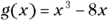
The following are some examples of functions and their ranges. Like domains, you can express ranges in words, inequalities, or interval notation (see Chapter 2):
 . The range of this function consists of the number 3 and any number greater than 3. You write the range as
  or, in interval notation,
  . The outputs can never be less than 3 because the numbers you input are squared. The result of squaring a real number is always positive (or if you input zero, you square zero). If you add a positive number or 0 to 3, you never get anything smaller than 3.
 . The range of this function consists of all positive numbers and zero. You write the range as
  or, in interval notation,
  . The number under the radical can never be negative, and all the square roots come out positive or zero.
 . Some functions’ equations, such as this one, don’t give an immediate clue to the range values. It often helps to sketch the graphs of these functions. Figure 6-1 shows the graph of the function p. See if you can figure out the range values before peeking at the following explanation.

John Wiley & Sons, Inc.
FIGURE 6-1: Try graphing equations that don’t have an obvious range.
The graph of this function never touches the x-axis, but it gets very close. For the numbers in the domain bigger than five, the graph has some really high y-values and some y-values that get really close to zero. But the graph never touches the x-axis, so the function value never really reaches zero. For numbers in the domain smaller than five, the curve is below the x-axis. These function values are negative — some really small. But, again, the y-values never reach zero. So, if you guessed that the range of the function is every real number except zero, you’re right! You write the range as ![]() , or
, or ![]() . Did you also notice that the function doesn’t have a value when
. Did you also notice that the function doesn’t have a value when ![]() ? This happens because 5 isn’t in the domain.
? This happens because 5 isn’t in the domain.
 When a function’s range has a lowest or highest value, it presents a case of an absolute minimum or an absolute maximum. For instance, if the range is
 ![]() , the range includes the number 2 and every value bigger than 2. The absolute minimum value that the function can output is 2. Not all functions have these absolute minimum and maximum values, but being able to identify them is important — especially if you use functions to determine your weekly pay. Do you want a cap on your pay at the absolute maximum of $500?
, the range includes the number 2 and every value bigger than 2. The absolute minimum value that the function can output is 2. Not all functions have these absolute minimum and maximum values, but being able to identify them is important — especially if you use functions to determine your weekly pay. Do you want a cap on your pay at the absolute maximum of $500?
 For some tips on how to graph functions, head to Chapters 7 through 10, where I discuss the graphs of the different kinds of functions.
Betting on Even or Odd Functions
You can classify numbers as even or odd (and you can use this information to your advantage; for example, you know you can divide even numbers by two and come out with a whole number). You can also classify some functions as even or odd. The even and odd integers (like 2, 4, 6, and 1, 3, 5) play a role in this classification, but they aren’t the be-all and end-all. You have to put a bit more calculation work into classifying the functions. If you didn’t have to put in the extra effort, you would’ve mastered this stuff in third grade, and I’d have nothing to write about.
Recognizing even and odd functions
An even function is one in which both a domain value (an input) and its opposite result in the same range value (output) — so, ![]() . An odd function is one in which a domain value and its opposite produce opposite results in the range — meaning,
. An odd function is one in which a domain value and its opposite produce opposite results in the range — meaning, ![]() .
.
To determine if a function is even or odd (or neither), you replace every x in the function equation with ![]() and simplify. If the function is even, the result in the simplified version looks exactly like the original. If the function is odd, the result in the simplified version looks like what you get after multiplying the original function equation by
and simplify. If the function is even, the result in the simplified version looks exactly like the original. If the function is odd, the result in the simplified version looks like what you get after multiplying the original function equation by ![]() .
.
The descriptions for even and odd functions may remind you of how even and odd numbers for exponents act (see Chapter 10). If you raise ![]() to an even power, you get a positive number:
to an even power, you get a positive number: ![]() . If you raise
. If you raise ![]() to an odd power, you get a negative (opposite) result:
to an odd power, you get a negative (opposite) result: ![]() .
.
The following are examples of some even and odd functions, and I explain how you label them so you can master the practice on your own:
 is even, because whether you input 2 or
  , you get the same output:
This is just a demonstration of how one pair of numbers works. To show that the function is even for any input value, you replace x with –x in the function rule:
 . This result is the original function — it must be even.
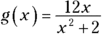 is odd, because the inputs 2 and
  give you opposite answers:
To show that this result happens for all pairs of input values, replace x with –x in the function rule.
 . This is the same as multiplying the original function rule by
  . The function must be odd.

You can’t say that a function is even just because it has even exponents and coefficients, and you can’t say that a function is odd just because the exponents and coefficients are odd numbers. If you do make these assumptions, you classify the functions incorrectly, which messes up your graphing. You have to apply the rules to determine which label a function has.
Applying even and odd functions to graphs
The biggest distinction between even and odd functions is how their graphs look:
- Even functions: The graphs of even functions are symmetric with respect to the y-axis (the vertical axis). You see what appears to be a mirror image to the left and right of the vertical axis. For an example of this type of symmetry, see Figure 6-2a, which is the graph of the even function

- Odd functions: The graphs of odd functions are symmetric with respect to the origin. The symmetry is radial, or circular, so it looks the same if you rotate the graph by 180 degrees. The graph in Figure 6-2b, which is the odd function
 , displays origin symmetry.

John Wiley & Sons, Inc.
FIGURE 6-2: Graphs of an even and an odd function.
You may be wondering whether you can have symmetry with respect to the x-axis. After all, is the y-axis all that better than the x-axis? I’ll leave that up to you, but yes, x-axis symmetry does exist — just not in the world of functions. By its definition, a function can have only one y value for every x value. If you have points on either side of the x-axis, above and below an x value, you don’t have a function. Head to Chapter 11 if you want to see some pictures of curves that are symmetric all over the place.
Facing One-to-One Confrontations
Functions can have many classifications or names, depending on the situation (maybe you want to model a business transaction or use them to figure out payments and interest) and what you want to do with them (put the formulas or equations in spreadsheets or maybe just graph them, for example). One very important classification is deciding whether a function is one-to-one.
Defining one-to-one functions
 A function is one-to-one if it has exactly one output value for every input value and exactly one input value for every output value. Formally, you write this definition as follows:
If
, then
In simple terms, if the two output values of a function are the same, then the two input values must also be the same.
One-to-one functions are important because they’re the only functions that can have inverses, and functions with inverses aren’t all that easy to come by. If a function has an inverse, you can work backward and forward — find an answer if you have a question and find the original question if you know the answer (sort of like Jeopardy!). For more on inverse functions, see the section “Singing Along with Inverse Functions” later in this chapter.
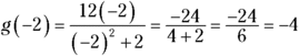
An example of a one-to-one function is ![]() . The rule for the function involves cubing the variable. The cube of a positive number is positive, and the cube of a negative number is negative. Therefore, every input has a unique output — no other input value gives you that output.
. The rule for the function involves cubing the variable. The cube of a positive number is positive, and the cube of a negative number is negative. Therefore, every input has a unique output — no other input value gives you that output.
Some functions without the one-to-one designation may look like the previous example, which is one-to-one. Take ![]() , for example. This counts as a function because only one output comes with every input. However, the function isn’t one-to-one, because you can create many outputs or function values from more than one input. For instance,
, for example. This counts as a function because only one output comes with every input. However, the function isn’t one-to-one, because you can create many outputs or function values from more than one input. For instance, ![]() , and
, and ![]() . You have two inputs, 1 and
. You have two inputs, 1 and ![]() , that result in the same output of 0.
, that result in the same output of 0.
Functions that don’t qualify for the one-to-one label can be hard to spot, but you can rule out any functions with all even-numbered exponents right away. Functions with absolute value usually don’t cooperate either.
Eliminating one-to-one violators
You can determine which functions are one-to-one and which are violators by sleuthing (guessing and trying), using algebraic techniques, and graphing. Most mathematicians prefer the graphing technique because it gives you a nice, visual answer. The basic graphing technique is the horizontal line test. But, to better understand this test, you need to meet its partner, the vertical line test. (I show you how to graph various functions in Chapters 7 through 10.)
Vertical line test
The graph of a function always passes the vertical line test. The test stipulates that any vertical line drawn through the graph of the function passes through that function no more than once. This is a visual illustration that only one y value (output) exists for every x value (input), a rule of functions. Figure 6-3a shows a function that passes the vertical line test, and Figure 6-3b contains a curve that isn’t a function and therefore flunks the vertical line test.

John Wiley & Sons, Inc.
FIGURE 6-3: A function passes the vertical line test, but a non-function inevitably fails.
Horizontal line test
All functions pass the vertical line test, but only one-to-one functions pass the horizontal line test. With this test, you can see if any horizontal line drawn through the graph cuts through the function more than one time. If the line passes through the function more than once, the function fails the test and therefore isn’t a one-to-one function. Figure 6-4a shows a function that passes the horizontal line test, and Figure 6-4b shows a function that flunks it.

John Wiley & Sons, Inc.
FIGURE 6-4: The horizontal line test weeds out one-to-one functions from violators.
Both graphs in Figure 6-4 are functions, however, so they both pass the vertical line test.
Going to Pieces with Piecewise Functions
A piecewise function consists of two or more function rules (function equations) pieced together (listed separately for different x-values) to form one bigger function. A change in the function equation occurs for different values in the domain. For example, you may have one rule for all the negative numbers, another rule for numbers bigger than three, and a third rule for all the numbers between those two rules.
Piecewise functions have their place in situations where you don’t want to use the same rule for everyone or everything. Should a restaurant charge a 3-year-old the same amount for a meal as it does an adult? Do you put on the same amount of clothing when the temperature is 20 degrees as you do in hotter weather? No, you place different rules on different situations. In mathematics, the piecewise function allows for different rules to apply to different numbers in the domain of a function.
Doing piecework
Piecewise functions are often rather contrived. Oh, they seem real enough when you pay your income tax or figure out your sales commission. But in an algebra discussion, it seems easier to come up with some nice equations to illustrate how piecewise functions work and then introduce the applications later. The following is an example of a piecewise function:

With this function, you use one rule for all numbers smaller than or equal to ![]() , another rule for numbers between
, another rule for numbers between ![]() and 3 (including the 3), and a final rule for numbers larger than 3. You still have only one output value for every input value. For instance, say you want to find the values of this function for x equaling
and 3 (including the 3), and a final rule for numbers larger than 3. You still have only one output value for every input value. For instance, say you want to find the values of this function for x equaling ![]() , and 5. Notice how you use the different rules depending on the input value:
, and 5. Notice how you use the different rules depending on the input value:
Figure 6-5 shows you the graph of the piecewise function with these function values.

John Wiley & Sons, Inc.
FIGURE 6-5: Graphing piecewise functions shows you both connections and gaps.
Notice the three different sections to the graph. The left curve and the middle line don’t connect because a discontinuity exists when ![]() . A discontinuity occurs when a gap or hole appears in the graph. Also, notice that the left line falling toward the x-axis ends with a solid dot, and the middle section has an open circle just above it. These features preserve the definition of a function — only one output for each input. The dot tells you to use the rule on the left when
. A discontinuity occurs when a gap or hole appears in the graph. Also, notice that the left line falling toward the x-axis ends with a solid dot, and the middle section has an open circle just above it. These features preserve the definition of a function — only one output for each input. The dot tells you to use the rule on the left when ![]() .
.
The middle section connects at point (3, 2) because the rule on the right gets really, really close to the same output value as the rule in the middle when ![]() . Technically, you should draw both a hollow circle and a dot, but you really can’t spot this feature just by looking at it.
. Technically, you should draw both a hollow circle and a dot, but you really can’t spot this feature just by looking at it.
Applying piecewise functions
Why in the world would you need to use a piecewise function? Do you have any good reason to change the rules right in the middle of things? I have two examples that aim to ease your mind — examples that you may relate to very well.
Utilizing a utility
Utility companies can use piecewise functions to charge different rates for users based on consumption levels. A big factory uses a ton of electricity and rightfully gets a different rate than a homeowner. Here’s what the company Lightning Strike Utility uses to figure the charges for its customers:
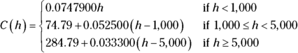
where h is the number of kilowatt hours and C is the cost in dollars.
So, how much does a homeowner who uses 750 kilowatt hours pay? How much does a business that uses 10,000 kilowatt hours pay?
You use the top rule for the homeowner and the bottom rule for the business, determined by what interval the input value lies in. The homeowner has the following equation:
The person using 750 kilowatt hours pays a little more than $56 per month. And the business?
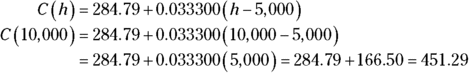
The company pays a little more than $451.
Taxing the situation
As April 15 rolls around, many people are faced with their annual struggle with income tax forms. The rate at which you pay tax is based on how much your adjusted income is — a graduated scale where (supposedly) people who make more money pay more income tax. The income values are the inputs (values in the domain), and the government determines the tax paid by putting numbers into the correct formula.
In 2014, a single taxpayer paid her income tax based on her taxable income, according to the following rules (laid out in a piecewise function):

where n is the taxable income and T is the tax paid.
If her taxable income was $45,000, how much did she pay in taxes? Insert the value and follow the third rule, because 45,000 is between 36,900 and 89,350:
This person paid a little more than $7,100 in income tax.
Composing Yourself and Functions
You can perform the basic mathematical operations of addition, subtraction, multiplication, and division on the equations used to describe functions. ( You can also perform whatever simplification is possible on the different parts of the expression and write the result as a new function.) For example, you can take the two functions ![]() and
and ![]() and perform the four operations on them:
and perform the four operations on them:
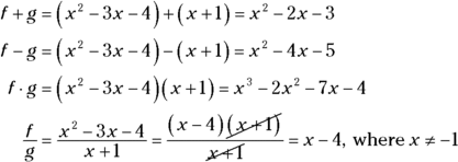
Well done, but you have another operation at your disposal — an operation special to functions — called composition.
Performing compositions
No, I’m not switching the format to a writing class. The composition of functions is an operation in which you use one function as the input into another and perform the operations on that input function.
You indicate the composition of functions f and g with a small circle between the function names, ![]() , and you define the composition as
, and you define the composition as ![]() .
.
Here’s how you perform an example composition, using the functions f and g from the preceding section, ![]() and
and ![]() :
:

The composition of functions isn’t commutative (addition and multiplication are commutative, because you can switch the order and not change the result). The order in which you perform the composition — which function comes first — matters. The composition ![]() isn’t the same as
isn’t the same as ![]() , save one exception: when the two functions are inverses of one another (see the section “Singing Along with Inverse Functions” later in this chapter).
, save one exception: when the two functions are inverses of one another (see the section “Singing Along with Inverse Functions” later in this chapter).
Simplifying the difference quotient
The difference quotient shows up in most high school Algebra II classes as an exercise you do after your instructor shows you the composition of functions. You perform this exercise because the difference quotient is the basis of the definition of the derivative. The difference quotient allows you to find the derivative, which allows you to be successful in calculus (because everyone wants to be successful in calculus, of course). So, where does the composition of functions come in? With the difference quotient, you do the composition of some designated function f (x) and the function ![]() or
or ![]() , depending on what calculus book you use.
, depending on what calculus book you use.
The difference quotient for the function f is ![]() . Yes, you have to memorize it.
. Yes, you have to memorize it.
Now, for an example, perform the difference quotient on the same function f from the previous section, ![]() :
:
Notice that you find the expression for ![]() by putting
by putting ![]() in for every x in the function —
in for every x in the function — ![]() is the input variable. Now, continuing on with the simplification:
is the input variable. Now, continuing on with the simplification:
Did you notice that ![]() , 3x, and 4 all appear in the numerator with their opposites? That’s why they disappear with the simplification. Now, to finish:
, 3x, and 4 all appear in the numerator with their opposites? That’s why they disappear with the simplification. Now, to finish:
Now, this may not look like much to you, but you’ve created a wonderful result. You’re one step away from finding the derivative. Tune in next week at the same time … no, I lied. You need to look at Calculus For Dummies, by Mark Ryan (Wiley), if you can’t stand the wait and really want to find the derivative. For now, you’ve just done some really decent algebra.
Singing Along with Inverse Functions
Some functions are inverses of one another, but a function can have an inverse only if it’s one-to-one (see the section “Facing One-to-One Confrontations” earlier in this chapter if you need a refresher). If two functions are inverses of one another, each function undoes what the other creates. In other words, you use them to get back where you started.
The notation for inverse functions is the exponent ![]() written after the function name. The inverse of function f (x), for example, is
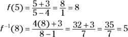
written after the function name. The inverse of function f (x), for example, is ![]() . Here are two functions that are inverses of one another and how they undo what the other did:
. Here are two functions that are inverses of one another and how they undo what the other did:
and
If you put 5 into function f, you get 8 as a result. If you put 8 into ![]() , you get 5 as a result — you’re back where you started:
, you get 5 as a result — you’re back where you started:
Now, what was the question? How can you tell with the blink of an eye when functions are inverses? Read on!
Determining if functions are inverses
In an example from the intro to this section, I tell you that two functions are inverses and then demonstrate how they work. You can’t really prove that two functions are inverses by plugging in numbers, however. You may face a situation where a couple of numbers work, but, in general, the two functions aren’t really inverses.
The only way to be sure that two functions are inverses of one another is to use the following general definition: Functions f and ![]() are inverses of one another only if
are inverses of one another only if ![]() and
and ![]() .
.
In other words, you have to do the composition in both directions (do ![]() and then do
and then do ![]() , which is the opposite order) and show that both result in the single value x.
, which is the opposite order) and show that both result in the single value x.
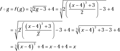
For some practice, show that ![]() and
and ![]() are inverses of one another. First, you perform the composition
are inverses of one another. First, you perform the composition ![]() :
:
Now you perform the composition in the opposite order:
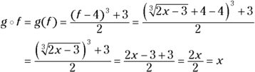
Both come out with a result of x, so the functions are inverses of one another.
Solving for the inverse of a function
Up until now in this section, I’ve given you two functions and told you that they’re inverses of one another. How did I know? Was it magic? Did I pull the functions out of a hat? No, you have a nice process to use. I can show you my secret so you can create all sorts of inverses for all sorts of functions. Lucky you! The following list gives you the step-by-step process that I use (more memorization to come).
To find the inverse of the one-to-one function f (x), follow these steps:
- Rewrite the function, replacing f (x) with y to simplify the notation.
- Change each y to an x and each x to a y.
- Solve for y.
- Rewrite the function, replacing the y with
 .
.
Here’s an example of how you work it. Find the inverse of the function ![]() :
:
- Rewrite the function, replacing f (x) with y to simplify the notation.

- Change each y to an x and each x to a y.

Solve for y.
Start by multiplying each side of the equation by the denominator and distributing.

Now subtract y from each side and add 5x to each side to get the terms with y in them on one side. Factor out that y.

Divide each side by
 .
.
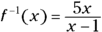
- Rewrite the function, replacing the y with
 .
.
This process helps you find the inverse of a function, if it has one. If you can’t solve for the inverse, the function may not be one-to-one to begin with. For instance, if you try to solve for the inverse of the function ![]() , you get stuck when you have to take a square root and don’t know if you want a positive or negative root. These are the kinds of roadblocks that alert you to the fact that the function has no inverse — and that the function isn’t one-to-one.
, you get stuck when you have to take a square root and don’t know if you want a positive or negative root. These are the kinds of roadblocks that alert you to the fact that the function has no inverse — and that the function isn’t one-to-one.