Interpreting relative value and absolute value

As I introduce in Chapter 5, many functions can have an absolute maximum or an absolute minimum value — the point at which the graph of the function has no higher or lower value, respectively. For example, a parabola opening downward has an absolute maximum — you see no point on the curve that’s higher than the maximum. In other words, no value of the function is greater than that number. (Check out Chapter 6 for more on quadratic functions and their parabola graphs.) Some functions, however, also have relative maximum or minimum values:

• Relative maximum: A point on the graph — a value of the function — that’s relatively large; the point is higher than anything around it, but you may be able to find a higher point somewhere else on the graph.
• Relative minimum: A point on the graph — a value of the function — that’s lower than anything close to it; it’s lower relative to all the points on the curve near it.

In Figure 8-1, you can see five turning points. Two are relative maximum values, which means they’re higher than any points close to them. Three are minimum values, which means they’re lower than any points around them. Two of the minimums are relative minimum values, and one is absolutely the lowest point on the curve. This function has no absolute maximum value because it keeps going up and up without end.

Counting intercepts and turning points

The number of potential turning points and x-intercepts of a polynomial function is good to know when you’re sketching the graph of the function. You can count the number of x-intercepts and turning points of a polynomial if you have the graph of it in front of you, but you can also make an estimate of the number if you have the equation of the polynomial. Your estimate is actually a number that represents the most points that can occur. You can say, “There are at most n intercepts and at most m turning points.” The estimate is the best you can do, but that’s usually not a bad thing.

To determine the rules for the greatest number of possible intercepts and greatest number of possible turning points from the equation of a polynomial, you look at the general form of a polynomial function.

Given the polynomial , the maximum number of x-intercepts is n, the degree or highest power of the polynomial. The maximum number of turning points is , or one less than the number of possible intercepts. You may find fewer intercepts than n, or you may find exactly that many.

If n is an odd number, you know right away that you have to find at least one x-intercept. If n is even, you may not find any x-intercepts.

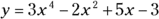
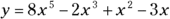
Examine the following two function equations as examples of polynomials. To determine the possible number of intercepts and turning points for the functions, look for the values of n, the exponents that have the highest values:

This graph has at most seven x-intercepts (7 is the highest power in the function) and six turning points .

This graph has at most six x-intercepts and five turning points.

You can see the graphs of these two functions in Figure 8-2. According to its function, the graph of the first example (Figure 8-2a) could have at least seven x-intercepts, but it has only five; it does have all six turning points, though. You can also see that two of the intercepts are touch-and-go types, meaning that they approach the x-axis before heading away again. The graph of the second example (Figure 8-2b) can have at most six x-intercepts, but it has only two; it does have all five turning points.

Figure 8-3 provides you with two extreme polynomial examples. The graphs of (Figure 8-3a) and (Figure 8-3b) seem to have great possibilities … that don’t pan out. The graph of , according to the rules of polynomials, could have as many as eight intercepts and seven turning points. But, as you can see from the graph, it has no intercepts and just one turning point. The graph of has only one intercept and no turning points.

The moral to the story of Figure 8-3 is that you have to use the rules of polynomials wisely, carefully, and skeptically. Also, think about the basic graphs of polynomials. The graphs are gently rolling curves that go from the left to the right across your graph. They cross the y-axis exactly once and may or may not cross the x-axis. You get hints from the standard equation of the polynomial and from the factored form. Refer to Chapter 5 if you need to review them.

Solving for polynomial intercepts

You can easily solve for the y-intercept of a polynomial function, of which you can find only one. The y-intercept is where the curve of the graph crosses the y-axis, and that’s when . So, to determine the y-intercept for any polynomial, simply replace all the x’s with zeros and solve for y (that’s the y part of the coordinate of that intercept):

• 
• When ,
• The y-intercept is .
• 
• When ,
• The y-intercept is (0, 0), at the origin.

After you complete the easy task of solving for the y-intercept, you find out that the x-intercepts are another matter altogether. The value of y is zero for all x-intercepts, so you let and solve for x.

Here, however, you don’t have the advantage of making everything disappear except the constant number like you do when solving for the y-intercept. When solving for the x-intercepts, you may have to factor the polynomial or perform a more elaborate process — techniques you can find later in this chapter in the section “Factoring for polynomial roots” or “Saving your sanity: The Rational Root Theorem,” respectively. For now, just apply the process of factoring and setting the factored form equal to zero to some carefully selected examples. This is essentially using the multiplication property of zero — setting the factored form equal to zero to find the intercepts (see Chapter 1).

To determine the x-intercepts of the following three polynomials, replace the y’s with zeros and solve for the x’s:

• 
• When , , , (using the square root rule from Chapter 3)
• 
• When , , (using the multiplication property of zero from Chapter 1)
• 
• When , , or (using the multiplication property of zero)

Both of these intercepts come from multiple roots (when a solution appears more than once). Another way of writing the factored form is

You could list the answer as . The number of times a root repeats is significant when you’re graphing. A multiple root has a different kind of look or graph where it intersects the axis. (For more, head to the section “Changing from roots to factors” later in this chapter.)

Using a sign-line

If you’re a visual person like me, you’ll appreciate the interval method I present in this section. Using a sign-line and marking the intervals between x-values allows you to determine where a polynomial is positive or negative, and it appeals to your artistic bent!

The function , for example, changes sign at every intercept. Setting and solving, you find that the x-intercepts are at . Now you can put this information about the problem to work.

To determine the positive and negative intervals for a polynomial function, follow this method:

1. Draw a number line, and place the values of the x-intercepts in their correct positions on the line.

   

2. Choose random values to the right and left of the intercepts to test whether the function is positive or negative in those positions.

   If the function equation is factored, you determine whether each factor is positive or negative, and you find the sign of the product of all the factors.

   Some possible random number choices are , and 8. These values represent numbers in each interval determined by the intercepts. (Note: These aren’t the only possibilities; you can pick your favorites.)

   . You don’t need the actual number value, just the sign of the result, so .

   , so .

   , so .

   , so .

   , so .

   You need to check only one point in each interval; the function values all have the same sign within that interval.

3. Place a or symbol in each interval to show the function sign.

   

   The graph of this function is positive, or above the x-axis, whenever x is smaller than , between 0 and 2, and bigger than 7. You write that when: or or . In interval notation, that’s .

The function doesn’t change at each intercept. The intercepts are where .

1. Draw the number line and insert the intercepts.

   

2. Test values to the left and right of each intercept. Some possible random choices are to let .

   When you can, you should always use 0, because it combines so nicely.

   is .

   is .

   is .

   is .

3. Mark the signs in the appropriate places on the number line.

   

   You probably noticed that the factors raised to an even power were always positive. The factor raised to an odd power is only positive when the result in the parentheses is positive.

Interpreting the rule

Look back at the two polynomial examples in the previous section. Did you notice that in the first example, the sign changed every time, and in the second, the signs were sort of stuck on the same sign for a while? When the signs of functions don’t change, the graphs of the polynomials don’t cross the x-axis at any intercepts, and you see touch-and-go graphs. Why do you suppose this is? First, look at graphs of two functions from the previous section in Figures 8-4a and 8-4b, and .

The rule for whether a function displays sign changes or not at the intercepts is based on the exponent on the factor that provides you with a particular intercept.

If a polynomial function is factored in the form , you see a sign change whenever is an odd number (meaning it crosses the x-axis), and you see no sign change whenever is even (meaning the graph of the function is touch and go; see the section “Exploring Polynomial Intercepts and Turning Points”).

So, for example, with the function , shown in Figure 8-5a, you see a sign change at and no sign change at . With the function , shown in Figure 8-5b, you never see a sign change.

Factoring for polynomial roots

Finding x-intercepts of polynomials isn’t difficult — as long as you have the polynomial in nicely factored form. You just set the y equal to zero and use the multiplication property of zero (see Chapter 1) to pick the intercepts off like flies. But what if the polynomial isn’t in factored form (and it should be)? What do you do? Well, you factor it, of course. This section deals with easily recognizable factors of polynomials — types that probably account for 70 percent of any polynomials you’ll have to deal with. (I cover other, more challenging types in the following sections.)

Applying factoring patterns and groupings

Half the battle is recognizing the patterns in factorable polynomial functions. You want to take advantage of the patterns. If you don’t see any patterns (or if none exist), you need to investigate further. The most easily recognizable factoring patterns used on polynomials are the following (which I brush up on in Chapter 1):

	Difference of squares
	Greatest common factor
	Difference of cubes
	Sum of cubes
	Perfect square trinomial
UnFOIL	Trinomial factorization
Grouping	Common factors in groups

The following examples incorporate the different methods of factoring. They contain perfect cubes and squares and all sorts of good combinations of factorization patterns.

To factor the following polynomial, for example, you should use the greatest common factor and then the difference of squares:

This polynomial requires factoring, using the sum of two perfect cubes:

You initially factor the next polynomial by grouping. The first two terms have a common factor of , and the second two terms have a common factor of . The terms in the new equation have a common factor of . After performing the factorization, you see that the first factor is the difference of squares and the second is the difference of cubes:

This last polynomial shows how you first use the greatest common factor and then factor with a perfect square trinomial:

Saving your sanity: The Rational Root Theorem

What do you do if the factorization of a polynomial doesn’t leap out at you? You have a feeling that the polynomial factors, but the necessary numbers escape you. Never fear! Your faithful author has just saved your day. My help is in the form of the Rational Root Theorem. This theorem is really neat because it’s so orderly and predictable, and it has an obvious end to it; you know when you’re done so you can stop looking for solutions. But before you can put the theorem into play, you have to be able to recognize a rational root — or a rational number, for that matter.

A rational number is any real number that you can write as a fraction with one integer divided by another. (An integer is a positive or negative whole number or zero.) You often write a rational number in the form , with the understanding that the denominator, q, can’t equal zero. All whole numbers are rational numbers because you can write them as fractions, such as .

What distinguishes rational numbers from their opposites, irrational numbers, has to do with the decimal equivalences. The decimal associated with a fraction (rational number) will either terminate or repeat (have a pattern of numbers that occurs over and over again). The decimal equivalent of an irrational number never repeats and never ends; it just wanders on aimlessly.

Without further ado, here’s the Rational Root Theorem: If the polynomial has any rational roots, they all meet the requirement that you can write them as a fraction equal to .

In other words, according to the theorem, any rational root of a polynomial is formed by dividing a factor of the constant term by a factor of the lead coefficient.

Putting the theorem to good use

The Rational Root Theorem gets most of its workout by letting you make a list of numbers that may be roots of a particular polynomial. After using the theorem to make your list of potential roots (and check it twice), you plug the numbers into the polynomial to determine which, if any, work. You may run across an instance where none of the candidates work, which tells you that there are no rational roots. (And if a given rational number isn’t on the list of possibilities that you come up with, it can’t be a root of that polynomial.)

Before you start to plug and chug, however, check out the section “Letting Descartes make a ruling on signs,” later in this chapter. It helps you with your guesses. Also, you can refer to “Synthesizing Root Findings” for a quicker method than plugging in.

POLYNOMIALS WITH CONSTANT TERMS

To find the roots of the polynomial , for example, you test the following possibilities: and . These values are all the factors of the number 12. Technically, you divide each of these factors of 12 by the factors of the lead coefficient, but because the lead coefficient is 1 (as in ), dividing by that number won’t change a thing. Note: You ignore the signs, because the factors for both 12 and 1 can be positive or negative, and you find several combinations that can give you a positive or negative root. You find out the sign when you test the root in the function equation.

To find the roots of another polynomial, , you first list all the factors of 20: and . Now divide each of those factors by the factors of 6. You don’t need to bother dividing by 1, but you need to divide each by 2, 3, and 6:

You may have noticed some repeats in the previous list that occur when you reduce fractions. For instance, is the same as , and is the same as . Even though this looks like a mighty long list, between the integers and fractions, it still gives you a reasonable number of candidates to try out. You can check them off in a systematic manner.

POLYNOMIALS WITHOUT CONSTANT TERMS

When a polynomial doesn’t have a constant term, you first have to factor out the greatest power of the variable that you can. If you’re looking for the possible rational roots of , for example, and you want to use the Rational Root Theorem, you get nothing but zeros. You have no constant term — or you can say the constant is zero, so all the numerators of the fractions would be zero.

You can overcome the problem by factoring out the factor of . The factored out x gives you the root zero. Now you apply the Rational Root Theorem to the new polynomial in the parentheses to get the possible roots:

Letting Descartes make a ruling on signs

Rene Descartes was a French philosopher and mathematician. One of his contributions to algebra is Descartes’ Rule of Signs. This handy, dandy rule is a weapon in your arsenal for the fight to find roots of polynomial functions. If you pair this rule with the Rational Root Theorem from the previous section, you’ll be well equipped to succeed.

The Rule of Signs tells you how many positive and negative real roots you may find in a polynomial. A real number is just about any number you can think of. It can be positive or negative, rational or irrational. The only thing it can’t be is imaginary. (I cover imaginary numbers in Chapter 14 if you want to know more about them.)

Changing the function to count negative roots

Along with the positive roots (see the previous section), Descartes’ Rule of Signs deals with the possible number of negative roots of a polynomial. After you count the possible number of positive real roots, you combine that value to the number of possible negative real roots to make your guesses and solve the equation.

Descartes’ Rule of Signs (Part 2): The polynomial has at most n real roots. Find , and then count the number of times the sign changes in and call that value q. The value of q is the maximum number of negative roots of f. If the number of negative roots isn’t q, the number is , , and so on, for as many multiples of two as necessary.

To determine the possible number of negative roots of the polynomial , for example, you first find by replacing each x with and simplifying:

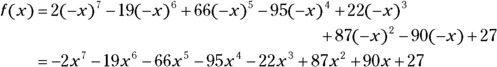
As you can see, the function has only one sign change, from negative to positive. Therefore, the function has exactly one negative root — no more, no less.

Knowing the potential number of positive and negative roots for a polynomial is very helpful when you want to pinpoint an exact number of roots. The example polynomial I present in this section has only one negative real root. That fact tells you to concentrate your guesses on positive roots; the odds are better that you’ll find a positive root first. When you’re using synthetic division (see the “Synthesizing Root Findings” section) to find the roots, the steps get easier and easier as you find and eliminate roots. By picking off the roots that you have a better chance of finding first, you can save the harder to find for the end.

Using synthetic division to test for roots

When you want to use synthetic division to test for roots in a polynomial, the last number on the bottom row of your synthetic division problem is the telling result. If that number is zero, the division had no remainder, and the number being tested is a root. The fact that there’s no remainder means that the binomial represented by the number is dividing the polynomial evenly. The number is a root because the binomial is a factor.

The polynomial , for example, has zeros or roots when . You could find as many as five real roots, which you can tell from the exponent 5 on the first x. Using Descartes’ Rule of Signs (see the previous section), you find two or zero positive real roots (indicated by the two sign changes). Replacing each x with , the polynomial now reads . Again, using the Rule of Signs, you find three or one negative real roots. (Counting up the number of positive and negative roots helps when you’re making a guess as to what a root may be.)

Now, using the Rational Root Theorem (see the section “Saving your sanity: The Rational Root Theorem”), your list of the potential rational roots is . You choose one of these and apply synthetic division.

You should generally go with the smaller numbers first, when using synthetic division, so use 1 and , 2 and , and so on.

Keeping in mind that smaller is better in this case, the following process shows a guess that is a root.

The steps for performing synthetic division on a polynomial to find its roots are as follows:

1. Write the polynomial in order of decreasing powers of the exponents. Replace any missing powers with zero to represent the coefficient.

   In this case, you’ve lucked out. The polynomial is already in the correct order: .

2. Write the coefficients in a row, including any zeros.
   

3. Put the number you want to divide by in front of the row of coefficients, separated by a half-box.

   In this case, the guess is .

   
4. Draw a horizontal line below the row of coefficients, leaving room for numbers under the coefficients.
   
5. Bring the first coefficient straight down below the line.
   
6. Multiply the number you bring below the line by the number that you’re dividing into everything. Put the result under the second coefficient.
   
7. Add the second coefficient and the product, putting the result below the line.
   
8. Repeat the multiplication/addition from Steps 6 and 7 with the rest of the coefficients.
   

The last entry on the bottom is a zero, so you know is a root. Now, you can do a modified synthetic division when testing for the next root; you just use the numbers across the bottom except the bottom right zero entry. (These values are actually coefficients of the quotient, if you do long division; see the following section.)

If your next guess is to see if is a root, the modified synthetic division appears as follows:

The last entry on the bottom row isn’t zero, so isn’t a root.

The really good guessers amongst you decide to try , , , and (a second time). These values represent the rest of the roots, and the synthetic division for all the guesses looks like this:

First, trying the ,

The last number in the bottom row is 0. That’s the remainder in the division. So now just look at all the numbers that come before the 0; they’re the new coefficients to divide into. Notice that the last coefficient is now 16, so you can modify your list of possible roots to be just the factors of 16. Also, they’re all positive with no sign changes. You don’t have any positive roots left. Now, dividing by :

In the next division, you consider only the negative factors of 4:

This time, dividing by ,

The last number in the row is 0, so is a root. Repeat the division, and you find that is a double root:

Your job is finished when you see the number one remaining in the last row, before the zero.

Now you can collect all the numbers that divided evenly — the roots of the equation — and use them to write the answer to the equation that’s set equal to zero or to write the factorization of the polynomial or to sketch the graph with these numbers as x-intercepts. In this case, the roots are and . The factorization (see the section “Changing from roots to factors” earlier in this chapter) is .

Synthetically dividing by a binomial

Finding the roots of a polynomial isn’t the only excuse you need to use synthetic division. You can also use synthetic division to replace the long, drawn-out process of dividing a polynomial by a binomial. Divisions like this are found in lots of calculus problems — where you need to make the expression more simplified so you can perform some wonderful operation.

The polynomial being divided can be any degree; the binomial has to be either or , and the coefficient on the x is 1. This may seem rather restrictive, but a huge number of long divisions you’d have to perform fit in this category, so it helps to have a quick, efficient method to perform these basic division problems.

To use synthetic division to divide a polynomial by a binomial, you first write the polynomial in decreasing order of exponents, inserting a zero for any missing exponent. The number you put in front or divide by is the opposite of the number in the binomial. So, if you divide by the binomial , you use in the synthetic division, as shown here:

As you can see, the last entry on the bottom row isn’t zero. If you’re looking for roots of a polynomial equation, this fact tells you that isn’t a root. In this case, because you’re working on a long division application (which you know because you need to divide to simplify the expression), the is the remainder of the division — in other words, the division doesn’t come out even.

You obtain the answer (quotient) of the division problem from the coefficients across the bottom of the synthetic division. You start with a power one value lower than the original polynomial’s power, and you use all the coefficients, dropping the power by one with each successive coefficient. The last coefficient is the remainder, which you write over the divisor.

Here’s the division problem and its solution. The original division problem is written first. After the problem, you see the coefficients from the synthetic division written in front of variables — starting with one degree lower than the original problem. The remainder of is written in a fraction on top of the divisor, .

Wringing out the Remainder (Theorem)

In the two previous sections, you use synthetic division to test for roots of a polynomial equation and then to do a long division problem. You use the same synthetic division process, but you read and use the results differently. In this section, I present yet another use of synthetic division involving the Remainder Theorem. When you’re looking for roots or solutions of a polynomial equation, you always want the remainder from the synthetic division to be zero. In this section, you get to see how to make use of all those pesky remainders that weren’t zeros.

The Remainder Theorem: When the polynomial is divided by the binomial , the remainder of the division is equal to f (c).

For instance, in the division problem from the previous section, has a remainder of . Therefore, according to the Remainder Theorem, for the function , .

The Remainder Theorem comes in very handy when finding function values because you’ll find it much easier to do synthetic division, where you multiply and add repeatedly, than to have to substitute numbers in for variables, raise the numbers to high powers, multiply by the coefficients, and then combine the terms.

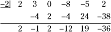
Using the Remainder Theorem to find f (3) when , for example, you apply synthetic division to the coefficients using 3 as the divider in the half-box.

The remainder of the division by is 83, and, by the Remainder Theorem, . Compare the process you use here with substituting the 3 into the function: . These numbers get really large. For instance, . The numbers are much more manageable when you use synthetic division and the Remainder Theorem.