Search in book...
Toggle Font Controls
Create new playlist

Name your new playlist

Playlist description (optional)
Sign In

Email address

Password

Forgot Password?

or

Continue with Facebook

Continue with Google
Sign Up

Full Name

Email address

Confirm Email Address

Password

or

Continue with Facebook

Continue with Google

Chapter 1

Going Beyond Beginning Algebra

IN THIS CHAPTER

Abiding by (and using) the rules of algebra

Adding the multiplication property of zero to your repertoire

Raising your exponential power

Looking at special products and factoring

Algebra is a branch of mathematics that people study before they move on to other areas or branches in mathematics and science. For example, you use the processes and mechanics of algebra in calculus to complete the study of change; you use algebra in probability and statistics to study averages and expectations; and you use algebra in chemistry to work out the balance between chemicals. Algebra all by itself is esthetically pleasing, but it springs to life when used in other applications.

Any study of science or mathematics involves rules and patterns. You approach the subject with the rules and patterns you already know, and you build on those rules with further study. The reward is all the new horizons that open up to you.

Any discussion of algebra presumes that you’re using the correct notation and terminology. Algebra I (check out Algebra I For Dummies [Wiley]) begins with combining terms correctly, performing operations on signed numbers, and dealing with exponents in an orderly fashion. You also solve the basic types of linear and quadratic equations. Algebra II gets into more types of functions, such as exponential and logarithmic functions, and topics that serve as launching spots for other math courses.

Going into a bit more detail, the basics of algebra include rules for dealing with equations, rules for using and combining terms with exponents, patterns to use when factoring expressions, and a general order for combining all the above. In this chapter, I present these basics so you can further your study of algebra and feel confident in your algebraic ability. Refer to these rules whenever needed as you investigate the many advanced topics in algebra.

Outlining Algebraic Properties

Mathematicians developed the rules and properties you use in algebra so that every student, researcher, curious scholar, and bored geek working on the same problem would get the same answer — no matter the time or place. You don’t want the rules changing on you every day (and I don’t want to have to write a new book every year!); you want consistency and security, which you get from the strong algebra rules and properties that I present in this section.

Keeping order with the commutative property

The commutative property applies to the operations of addition and multiplication. It states that you can change the order of the values in a particular operation without changing the final result:

If you add 2 and 3, you get 5. If you add 3 and 2, you still get 5. If you multiply 2 times 3, you get 6. If you multiply 3 times 2, you still get 6.

Algebraic expressions usually appear in a particular order, which comes in handy when you have to deal with variables and coefficients (multipliers of variables). The number part comes first, followed by the letters, in alphabetical order. But the beauty of the commutative property is that 2xyz is the same as x2zy. You have no good reason to write the expression in that second, jumbled order, but it’s helpful to know that you can change the order around when you need to.

Maintaining group harmony with the associative property

Like the commutative property (see the previous section), the associative property applies only to the operations of addition and multiplication. The associative property states that you can change the grouping of operations without changing the result:

You can use the associative property of addition or multiplication to your advantage when simplifying expressions. And if you throw in the commutative property when necessary, you have a powerful combination. For instance, when simplifying , you can start by dropping the parentheses (thanks to the associative property). You then switch the middle two terms around, using the commutative property of addition. You finish by reassociating the terms with parentheses and combining the like terms:

The steps in the previous process involve a lot more detail than you really need. You probably did the problem, as I first stated it, in your head. I provide the steps to illustrate how the commutative and associative properties work together; now you can apply them to more complex situations.

Distributing a wealth of values

The distributive property states that you can multiply each term in an expression within parentheses by the multiplier outside the parentheses and not change the value of the expression. It takes one operation, multiplication, and spreads it out over terms that you add to and subtract from one another:

For instance, you can use the distributive property on the problem to make your life easier. You distribute the 12 over the fractions by multiplying each fraction by 12 and then combining the results:

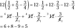
Finding the answer with the distributive property is much easier than changing all the fractions to equivalent fractions with common denominators of 12, combining them, and then multiplying by 12.

You can use the distributive property to simplify equations — in other words, you can prepare them to be solved. You also do the opposite of the distributive property when you factor expressions; see the section “Implementing Factoring Techniques” later in this chapter.

Checking out an algebraic ID

The numbers zero and one have special roles in algebra — as identities. You use identities in algebra when solving equations and simplifying expressions. You need to keep an expression equal to the same value, but you want to change its format, so you use an identity in one way or another:

Applying the additive identity

One situation that calls for the use of the additive identity is when you want to change the format of an expression so you can factor it. For instance, take the expression and add 0 to it. You get , which doesn’t do much for you (or me, for that matter). But how about replacing that 0 with both 9 and ? You now have , which you can write as and factor into . Why in the world do you want to do this? Go to Chapter 11 and read up on conic sections to see why. By both adding and subtracting 9, you add 0 — the additive identity.

Making multiple identity decisions

You use the multiplicative identity extensively when you work with fractions. Whenever you rewrite fractions with a common denominator, you actually multiply by one. If you want the fraction to have a denominator of 6x, for example, you multiply both the numerator and denominator by 3:

Now you’re ready to rock and roll with a fraction to your liking.

Singing along in-verses

You face two types of inverses in algebra: additive inverses and multiplicative inverses. The additive inverse matches up with the additive identity and the multiplicative inverse matches up with the multiplicative identity. The additive inverse is connected to zero, and the multiplicative inverse is connected to one.

A number and its additive inverse add up to zero. A number and its multiplicative inverse have a product of one. For example, and 3 are additive inverses; the multiplicative inverse of is . Inverses come into play big-time when you’re solving equations and want to isolate the variable. You use inverses by adding them to get zero next to the variable or by multiplying them to get one as a multiplier (or coefficient) of the variable.

Ordering Your Operations

When mathematicians switched from words to symbols to describe mathematical processes, their goal was to make dealing with problems as simple as possible; however, at the same time, they wanted everyone to know what was meant by an expression and for everyone to get the same answer to the same problem. Along with the special notation came a special set of rules on how to handle more than one operation in an expression. For instance, if you do the problem , you have to decide when to add, subtract, multiply, divide, take the root, and deal with the exponent.

The order of operations dictates that you follow this sequence:

Raise to powers or find roots.
Multiply or divide.
Add or subtract.

If you have to perform more than one operation from the same level, work those operations moving from left to right. If any grouping symbols appear, perform the operation inside the grouping symbols first.

So, to simplify , follow the order of operations:

The radical acts like a grouping symbol, so you subtract what’s in the radical first: .
Raise the power and find the root: .
Multiply and divide, working from left to right: .
Add and subtract, moving from left to right: .

Zeroing in on the Multiplication Property of Zero

You may be thinking that multiplying by zero is no big deal. After all, zero times anything is zero, right? Yes, and that’s the big deal. You can use the multiplication property of zero when solving equations. If you can factor an equation — in other words, write it as the product of two or more multipliers — you can apply the multiplication property of zero to solve the equation. The multiplication property of zero states that

If the product of , at least one of the factors has to represent the number 0.

The only way the product of two or more values can be zero is for at least one of the values to actually be zero. If you multiply (16)(467)(11)(9)(0), the result is 0. It doesn’t really matter what the other numbers are — the zero always wins.

The reason this property is so useful when solving equations is that if you want to solve the equation , for instance, you need the numbers that replace the x’s to make the equation a true statement. This particular equation factors into . The product of the four factors shown here is zero. The only way the product can be zero is if one or more of the factors is zero. For instance, if , the third factor is zero, and the whole product is zero. Also, if x is zero, the whole product is zero. (Head to Chapters 3 and 8 for more info on factoring and using the multiplication property of zero to solve equations.)

Expounding on Exponential Rules

Several hundred years ago, mathematicians introduced powers of variables and numbers called exponents. The use of exponents wasn’t immediately popular, however. Scholars around the world had to be convinced; eventually, the quick, slick notation of exponents won over, and we benefit from the use today. Instead of writing xxxxxxxx, you use the exponent 8 by writing . This form is easier to read and much quicker.

The expression is an exponential expression with a base of a and an exponent of n. The n tells you how many times you multiply the a times itself.

You use radicals to show roots. When you see , you know that you’re looking for the number that multiplies itself to give you 16. The answer? Four, of course. If you put a small superscript in front of the radical, you denote a cube root, a fourth root, and so on. For instance, , because the number 3 multiplied by itself four times is 81. You can also replace radicals with fractional exponents — terms that make them easier to combine. This use of exponents is very systematic and workable — thanks to the mathematicians who came before us.

Multiplying and dividing exponents

When two numbers or variables have the same base, you can multiply or divide those numbers or variables by adding or subtracting their exponents:

: When multiplying numbers with the same base, you add the exponents.
: When dividing numbers with the same base, you subtract the exponents (numerator – denominator). And, in this case, .

Also, recall that . Again, . To multiply , for example, you add the exponents: . When dividing by , you subtract the exponents: . You must be sure that the bases of the expressions are the same. You can multiply and , but you can’t use the rule of exponents when multiplying and .

Getting to the roots of exponents

Radical expressions — such as square roots, cube roots, fourth roots, and so on — appear with a radical to show the root. Another way you can write these values is by using fractional exponents. You’ll have an easier time combining variables with the same base if they have fractional exponents in place of radical forms:

: The root goes in the denominator of the fractional exponent.
: The root goes in the denominator of the fractional exponent, and the power goes in the numerator.

So, you can say and so on, along with .

To simplify a radical expression such as , you change the radicals to exponents and apply the rules for multiplication and division of values with the same base (see the previous section):

Raising or lowering the roof with exponents

You can raise numbers or variables with exponents to higher powers or reduce them to lower powers by taking roots. When raising a power to a power, you multiply the exponents. When taking the root of a power, you divide the exponents:

: Raise a power to a power by multiplying the exponents.
: Reduce the power when taking a root by dividing the exponents.

The second rule may look familiar — it’s one of the rules that govern changing from radicals to fractional exponents (see Chapter 4 for more on dealing with radicals and fractional exponents).

Here’s an example of how you apply the two rules when simplifying an expression:

Making nice with negative exponents

You use negative exponents to indicate that a number or variable belongs in the denominator of the term:

Writing variables with negative exponents allows you to combine those variables with other factors that share the same base. For instance, if you have the expression , you can rewrite the fractions by using negative exponents and then simplify by using the rules for multiplying factors with the same base (see “Multiplying and dividing exponents”):

Implementing Factoring Techniques

When you factor an algebraic expression, you rewrite the sums and differences of the terms as a product. For instance, you write the three terms in factored form as . The expression changes from three terms to one big, multiplied-together term. You can factor two terms, three terms, four terms, and so on for many different purposes. The factorization comes in handy when you set the factored forms equal to zero to solve an equation. Factored numerators and denominators in fractions also make it possible to reduce the fractions.

You can think of factoring as the opposite of distributing. You have good reasons to distribute or multiply through by a value — the process allows you to combine like terms and simplify expressions. Factoring out a common factor also has its purposes for solving equations and combining fractions. The different formats are equivalent — they just have different uses.

Factoring two terms

When an algebraic expression has two terms, you have four different choices for its factorization — if you can factor the expression at all. If you try the following four methods and none of them work, you can stop your attempt; you just can’t factor the expression:

In general, you check for a greatest common factor before attempting any of the other methods. By taking out the common factor, you often make the numbers smaller and more manageable, which helps you see clearly whether any other factoring is necessary.

To factor the expression , for example, you first factor out the common factor, 6x, and then you use the pattern for the difference of two perfect cubes:

A quadratic trinomial is a three-term polynomial with a term raised to the second power. When you see something like (as in this case), you immediately run through the possibilities of factoring it into the product of two binomials. In this case, you can just stop. These trinomials that crop up when factoring cubes just don’t cooperate.

Keeping in mind my tip to start a problem off by looking for the greatest common factor, look at the example expression . When you factor the expression, you first divide out the common factor, , to get . You then factor the difference of perfect squares in the parentheses: .

Here’s one more: The expression is the difference of two perfect squares. When you factor it, you get . Notice that the first factor is also the difference of two squares — you can factor again. The second term, however, is the sum of squares — you can’t factor it. With perfect cubes, you can factor both differences and sums, but not with the squares. So, the factorization of is .

Taking on three terms

When a quadratic expression has three terms, making it a trinomial, you have two different ways to factor it. One method is factoring out a greatest common factor, and the other is finding two binomials whose product is identical to those three terms:

You can often spot the greatest common factor with ease; you see a multiple of some number or variable in each term. With the product of two binomials, you either find the product or become satisfied that it doesn’t exist.

For example, you can perform the factorization of by dividing each term by the common factor, .

You want to look for the common factor first; it’s usually easier to factor expressions when the numbers are smaller. In the previous example, all you can do is pull out that common factor — the trinomial is prime (you can’t factor it any more).

Trinomials that factor into the product of two binomials have related powers on the variables in two of the terms. The relationship between the powers is that one is twice the other. When factoring a trinomial into the product of two binomials, you first look to see if you have a special product: a perfect square trinomial. If you don’t, you can proceed to unFOIL. The acronym FOIL helps you multiply two binomials (First, Outer, Inner, Last); unFOIL helps you factor the product of those binomials.

Finding perfect square trinomials

A perfect square trinomial is an expression of three terms that results from the squaring of a binomial — multiplying it times itself. Perfect square trinomials are fairly easy to spot — their first and last terms are perfect squares, and the middle term is twice the product of the roots of the first and last terms:

To factor , for example, you should first recognize that 20x is twice the product of the root of and the root of 100; therefore, the factorization is . An expression that isn’t quite as obvious is . You can see that the first and last terms are perfect squares. The root of is 5y, and the root of 9 is 3. The middle term, 30y, is twice the product of 5y and 3, so you have a perfect square trinomial that factors into .

Resorting to unFOIL

When you factor a trinomial that results from multiplying two binomials, you have to play detective and piece together the parts of the puzzle. Look at the following generalized product of binomials and the pattern that appears:

So, where does FOIL come in? You need to FOIL before you can unFOIL, don’t ya think?

The F in FOIL stands for “First.” In the previous problem, the First terms are the ax and cx. You multiply these terms together to get . The Outer terms are ax and d. Yes, you already used the ax, but each of the terms will have two different names. The Inner terms are b and cx; the Outer and Inner products are, respectively, adx and bcx. You add these two values. (Don’t worry; when you’re working with numbers, they combine nicely.) The Last terms, b and d, have a product of bd. Here’s an actual example that uses FOIL to multiply — working with numbers for the coefficients rather than letters:

Now, think of every quadratic trinomial as being of the form . The coefficient of the term, ac, is the product of the coefficients of the two x terms in the parentheses; the last term, bd, is the product of the two second terms in the parentheses; and the coefficient of the middle term is the sum of the outer and inner products. To factor these trinomials into the product of two binomials, you can use the opposite of the FOIL, which I call unFOIL.

Here are the basic steps you take to unFOIL the trinomial :

Determine all the ways you can multiply two numbers to get ac, the coefficient of the squared term.
Determine all the ways you can multiply two numbers to get bd, the constant term.
If the last term is positive, find the combination of factors from Steps 1 and 2 whose sum is that middle term; if the last term is negative, you want the combination of factors to be a difference.
Arrange your choices as binomials so that the factors line up correctly.
Insert the and signs to finish off the factoring and make the sign of the middle term come out right.

To factor , for example, you need to find two terms whose product is 20 and whose sum is 9. The coefficient of the squared term is 1, so you don’t have to take any other factors into consideration. You can produce the number 20 with , , or . The last pair is your choice, because . Arranging the factors and x’s into two binomials, you get .

Factoring four or more terms by grouping

When four or more terms come together to form an expression, you have bigger challenges in the factoring. You see factoring by grouping in the previous section as a method for factoring trinomials; the grouping is pretty obvious in this case. But what about when you’re starting from scratch? What happens with exponents greater than two? As with an expression with fewer terms, you always look for a greatest common factor first. If you can’t find a factor common to all the terms at the same time, your other option is grouping. To group, you take the terms two at a time and look for common factors for each of the pairs on an individual basis. After factoring, you see if the new groupings have a common factor. The best way to explain this is to demonstrate the factoring by grouping on and then on .

The four terms don’t have any common factor. However, the first two terms have a common factor of , and the last two terms have a common factor of 3:

Notice that you now have two terms, not four, and they both have the factor . Now, factoring out of each term, you have .

Factoring by grouping only works if a new common factor appears — the exact same one in each term.

The six terms don’t have a common factor, but, taking them two at a time, you can pull out the factors , , and . Factoring by grouping, you get the following: