The 3D Placement utilities generated by 3D and environment textures possess unique application traits. Projection utilities, on the other hand, are designed to work with 2D textures. Three-dimensional textures procedurally create a wide range of solid patterns; that is, they have height, width, and depth. In addition, you can convert 3D textures into 2D bitmaps with the Convert To File Texture tool.
Chapter Contents
Review and application of 3D textures
Attributes of 2D and 3D noise textures
Review of environment textures
Application of 2D texture Projection utilities
Strategies for placing placement boxes and projection icons
Maya 3D textures are procedural. That is, they are generated mathematically through predefined algorithms. Procedural textures are resolution independent and do not have defined edges or borders. Many of the algorithms employed by Maya make use of fractal math, which defines nonregular geometric shapes that have the same degree of nonregularity at all scales. Thus, Maya 3D textures are suitable for many shading scenarios found in the natural world. For example, the addition of 3D textures to a shading network can distress and dirty a clean floor and wall (see Figure 5.1).
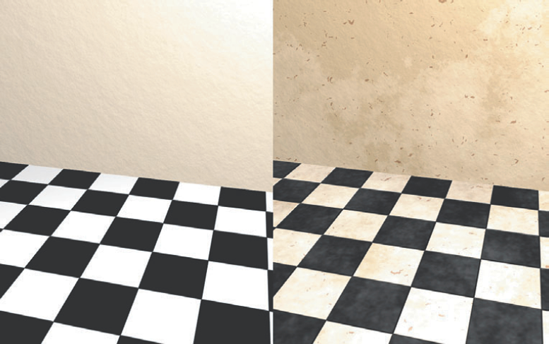
Figure 5.1. (Left) Set with standard textures. (Right) Same set with the addition of 3D textures to the shading networks. This scene is included on the CD as dirty_set.ma.
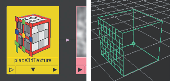
When you MMB-drag a 3D texture into the Hypershade work area or choose it through the Create Render Node window, a 3D Placement utility is automatically connected to the texture and named place3dTexture (see Figure 5.2). The scale, translation, and rotation of the 3D Placement utility's placement box affects the way in which the texture is applied to the assigned object. If the assigned object is scaled, translated, or rotated, it will pick up different portions of the texture. By default, new placement boxes are positioned at 0, 0, 0 in world space and are 2 × 2 × 2 units large. If the 3D Placement utility is deleted or its connection is broken, Maya assumes that the 3D texture sample is at its default size and position.
The 3D Placement utility determines the color of each surface point by locating the point's position within the placement box. Each position derives a potentially unique color. This process is analogous to a surface dipped into a square bucket of swirled paint or a surface chiseled from a solid cube of veined stone. Should the surface sit outside the placement box, the surface continues to receive a unique piece of the 3D texture. Since 3D textures are generated procedurally, there isn't a definitive texture border at the edge of the placement box. A significant advantage of 3D textures, and the use of the 3D Placement utility, is the disregard of a surface's UV texture space. In other words, the condition of a surface's UVs does not impact the ability of a 3D texture to map smoothly across the surface.
You can group Maya 3D textures, found in the 3D Textures section of the Create Maya Nodes menu in the Hypershade window, into four categories: random, natural, granular, and abstract.
Random 3D textures follow their 2D counterparts by attempting to produce a random, infinitely repeating pattern.
The Brownian texture is based on Brownian Motion, which is a mathematical model that describes the random motion of particles in a fluid dynamic system. A key element of the model is the "random walk," in which each successive step of a particle is in a completely random direction. Brownian Motion was discovered by the biologist Robert Brown (1773–1858).
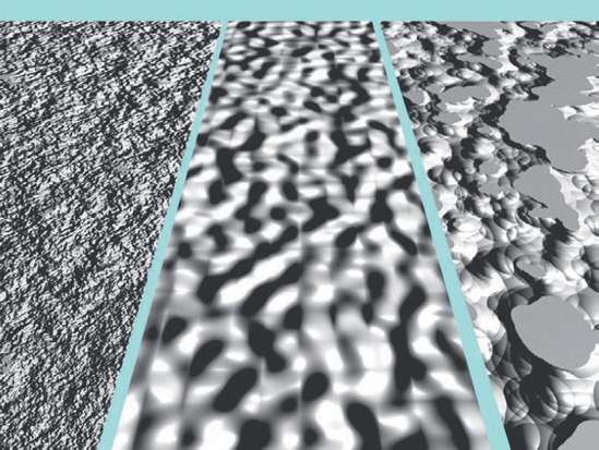
In general, the Brownian texture is smoother than other fractal-based textures. As such, the texture can replicate a sandy beach or similar surface. One disadvantage of the Brownian texture, however, is its tendency to produce rendering artifacts when viewed up close. For example, in Figure 5.3, a faint grid is visible on the middle plane.
The distinctive attributes of the Brownian texture follow:
- Lacunarity
Represents the gap between various noise frequencies. A higher value creates more detail. A lower value makes the texture smoother. Lacunarity, as a term, refers to the size and distribution of holes appearing in a fractal.
- Increment
Signifies the ratio of fractal noise used by the texture. A higher value reduces the contrast between light and dark areas.
- Octaves
Sets the number of calculation iterations. A higher value creates more detail in the map.
- Weight3d
Determines the internal fundamental frequency of the fractal pattern. A low value in the X, Y, or Z field causes the texture to smear in that particular direction.
The Volume Noise texture is a 3D variation of the Noise texture. The following attributes are shared by both Volume Noise and Noise:
- Threshold and Amplitude
The Threshold value is added to the colors produced by the fractal pattern, which raises all the color values present in the pattern. If any color value exceeds 1, it's clamped to 1. The colors produced by the fractal are also multiplied by the Amplitude value. If the Amplitude value is 1, the texture does not change. If the Amplitude value is 0.5, all the color values are halved.
Note
Noise and Fractal textures, at their default settings, often contain too much contrast to be useful in many situations. A quick way to reduce this contrast is to pull the Amplitude and Threshold sliders toward each other to the slider center.
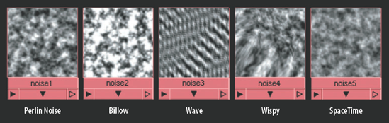
- Noise Type
There are five types of noise (see Figure 5.4). Billow is the default and contains sharper, disc-like blobs. Billow provides additional attributes, including Density, Spottyness, Size Rand, Randomness, and Falloff. Each of these attributes controls what its name implies. Perlin Noise uses Ken Perlin's classic 2D model, which produces a fairly soft pattern. Wave produces patterns similar to the Wave texture and will undulate if Time is animated. (The Wave noise type is listed as Volume Wave with the Volume Noise texture.) Num Waves sets the number of waves used by the Wave noise type. Wispy uses classic Perlin Noise but adds smeared distortions with a second noise layer. SpaceTime is a 3D version of classic Perlin Noise. Changing the Time attribute will select different 2D "slices" of SpaceTime noise.
- Ratio, Depth Max, and Frequency Ratio
Ratio controls the ratio of low- to high-frequency noise. If the value is 0, only low-frequency noise is visible. The low-frequency noise creates the large black and white noise "blobs." If the Ratio value is high, multiple layers of noise with higher and higher frequencies are added to the low frequency. The number of layers added depends on the Depth Max attribute. Depth Max controls the number of iterations the texture undertakes in its calculations and therefore determines the number of potential frequency layers. The higher the Depth Max value, the more complex the resulting noise. Frequency Ratio, on the other hand, establishes the scale of the frequencies involved in the Ratio calculation. Higher values create noise with finer detail.
- Inflection
If Inflection is checked, it inserts a mathematical "kink" into the noise function. In effect, this creates dark borders around various blobs of noise and injects white into the dark gaps. Inflection has no affect on the Billow noise type.
- Time
For the Noise texture, Time establishes which "slice" of the noise pattern is viewed. The Noise texture can be visualized as a 3D noise pattern from which 2D slices are retrieved. Each layer that is added with the Depth Max attribute is a slice from a noise pattern at a different frequency. The Time attribute creates a slightly different result for each Noise Type. For example, with Perlin Noise, higher Time values force Maya to choose a slice that is lower in the V direction and to the left in the U direction. With SpaceTime, higher values force Maya to choose a slice that is "deeper"; that is, raising the Time value moves the slice view "through" the three-dimensional noise.
You can see movement through the three-dimensional noise by keyframing the Time attribute. For example, in Figure 5.5 a cube is assigned to a Surface Shader material. A Volume Noise texture is mapped to the Out Color of the Surface Shader. The Noise Type attribute is set to SpaceTime. The Time attribute is animated, changing from 0 to 3 over 90 frames. Frequency Ratio is set to 1, Frequency is set to 4, and Scale is set to 5, 5, 5, making the pattern larger and easier to see.

Figure 5.5. Three frames from a Volume Noise texture with a keyframed Time attribute. This scene is included on the CD as
noise_slice.ma. A QuickTime movie is included asnoise_slice.mov.For the Volume Noise texture, Time establishes which section of the noise pattern, defined as a cube, is used. As with the Noise texture, the style of noise established by the Noise Type attribute affects the way in which Time moves across or through the 3D noise pattern.
- Frequency
Frequency defines the fundamental frequency of the noise. A high value "zooms out" from the texture. A low value "zooms in" to the texture. A value of 0 creates a dark gray. High values add detail to the noise.
- Implode and Implode Center
Implode warps the noise around a point defined by Implode Center. With the Noise texture, a high Implode value streaks the noise away from the viewer. A low value bulges the noise outward in a spherical fashion. With the Volume Noise texture, a high Implode value stretches the pattern or creates a wave-like warp depending on the Implode Center values. (If Implode Center is set to 0, 0, 0, Implode has no effect on Volume Noise.)
In addition, the Volume Noise texture has two unique attributes:
- Scale
Determines the scale of the noise in the X, Y, and Z directions. You can choose different values for each axis. For instance, a Scale of 1, 10, 1 stretches the noise detail in the Y direction.
- Origin
Offsets the noise in the X, Y, and Z directions. In other words, the cube that cuts out a section of the 3D noise pattern is moved through the noise to a new location.
Whether a Volume Noise or Noise texture should be selected depends on the nature of the object assigned to the texture's shading network. Since Volume Noise depends on a 3D Placement utility, it is not suited for an object that deforms or is in motion. On the other hand, the Noise texture, which is mapped directly to the surface, is restricted by the quality of the surface UVs. For example, in Figure 5.6 a polygon frog has a Noise and Volume Noise mapped to the Color attribute of an assigned Blinn material. In both cases, the Color Gain and Color Offset attributes of the noise texture are tinted green. Since the frog is split into multiple UV shells (groups of UV points), shell borders are noticeable on the Noise texture version. The Volume Noise version, by comparison, ignores the inherent UV information in favor of the 3D Placement process. Hence, the Volume Noise version renders cleanly with no shell borders. To improve the quality of the Noise version, more time must be spent refining the UVs. To make the Volume Noise version acceptable for animation and deformation, you must use the Convert To File Texture tool or the Transfer Maps window. (Convert To File Texture is described at the end of this chapter; the Transfer Maps window is discussed in Chapter 13.) The same dilemmas occur when choosing between Fractal and Solid Fractal textures.
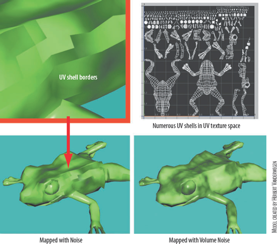
Figure 5.6. A polygon frog with Noise and Volume Noise textures mapped to the color of the assigned Blinn
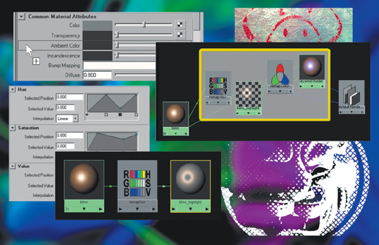
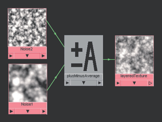
On a more technical level, Perlin Noise, and thus Noise and Volume Noise texture variations, are graphic representations of multiple noise functions, each at a different scale (frequency), added together. You can emulate the addition of noise functions in the Hypershade window by connecting two Noise textures to a Plus Minus Average utility. For example, in Figure 5.7 the Out Color attributes of two Noise textures are connected to input3D[0] and input3D[1] of a Plus Minus Average utility. The Operation of the utility is set to Average. To see the result, the utility's output3D is connected to a Layered Texture. The Layered Texture icon reveals a new, more complex noise pattern, which is a combination of Noise1 and Noise2. Noise1's Frequency is set to 3 and Noise2's Frequency is set to 10, guaranteeing that the scale of each noise pattern is different.
The Solid Fractal texture is a 3D variation of the Fractal texture. Both Solid Fractal and Fractal share attributes with Volume Noise and Noise. These attributes include Amplitude, Threshold, Ratio, Frequency Ratio, and Inflection. For descriptions of each attribute, see the previous section in this chapter. At the same time, Solid Fractal and Fractal share the following unique attributes:
- Bias
Controls the amount of contrast in the texture. A high value creates more contrast. A value of −1 creates a solid 50 percent gray.
- Animated
If checked, makes the Time and Time Ratio attributes available. Time retrieves different "slices" of the noise. With the default settings, slight variations in the Time value make changes to the noise pattern drastic and seemingly random (equivalent to television static). However, you can control the degree of change with the Time Ratio attribute. The lower the Time Ratio value, the more gradual the change to the noise pattern. To see a truly incremental change in the noise pattern, Time must be raised or lowered by less than 0.01 per frame and Time Ratio must be kept near 1. As with the SpaceTime noise type available for the Noise texture, the movement is through the noise pattern (as opposed to left to right or down to up).
In addition, the Fractal texture carries the Level Min and Level Max attributes. These two attributes control the number of iterations the texture undertakes in its calculations. A high Level Max value will produce finer detail in the resulting noise. Solid Fractal, on the other hand, carries the Ripples and Depth attributes. The Ripples fields, which represent Ripples X, Ripples Y, and Ripples Z attributes, control the fundamental noise frequency of the Solid Fractal. In basic terms, Ripples creates waviness in the texture in the X, Y, and Z directions. A high value in any one of the three fields causes the noise to stretch. High values in all three fields inserts a greater number of dark "holes" into the noise. The Depth fields, which represent Depth Min and Depth Max attributes, set the minimum and maximum number of iterations used in the Solid Fractal calculation. The higher the values, the finer the detail. The lower the values, the blurrier the texture.
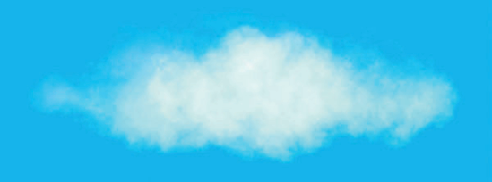
The Cloud texture uses Perlin and fractal noise techniques to create soft, wispy noise suitable for smoke or clouds. To create a cloud in a sky, follow these steps:
Create a NURBS sphere. Scale the sphere in one direction so that it becomes elongated.
Open the Hypershade window. MMB-drag a Lambert material into the work area. Assign the Lambert to the sphere.
Open the Lambert's Attribute Editor tab. Change the Color attribute to a suitable cloud color. Click the Transparency checkered Map button and choose the Cloud texture from the Create Render Node window.
With the Cloud texture open in the Attribute Editor, change Color1 and Color2 to 100 percent white. In the Effects section, select Invert. This ensures that the edges, and not the sphere's center, are transparent. Render a test frame. The sphere looks like a puff of smoke.
In the perspective workspace view, choose View > Camera Attribute Editor. The camera's Attribute Editor tab opens. In the Environment section, change Background Color to a more suitable sky color. Render a test frame.
Open the Cloud texture's Attribute Editor tab. To prevent the edges of the sphere from appearing too opaque or too black, incrementally raise the Edge Thresh attribute value. This erodes the cloud's edges so that a spherical outline can no longer be seen. Render a series of tests to check this. If the cloud appears too granular or noisy, lower the Ratio attribute slightly. This makes the noise pattern blurrier.
Open the Lambert's Attribute Editor tab. Slowly raise the Ambient Color until the majority of dark spots on the cloud disappear. Render a series of tests to check this.
Open the Cloud texture's Attribute Editor tab. Incrementally raise the Color Offset attribute in the Color Balance section. This thins the cloud and makes it appear more wispy (see Figure 5.8). Render a series of tests to check this. For additional realism, move the vertices of the sphere to make the resulting cloud's shape more random.
In addition, you can use the Cloud texture to quickly create a moon or other planetary body. For example, in Figure 5.9 a Cloud texture is mapped to the Incandescence of a Lambert material, which is assigned to a sphere.
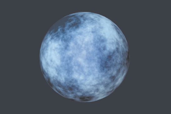
Figure 5.9. A Cloud texture is mapped to the Incandescence attribute of a Lambert material, creating a moonlike texture. This scene is included on the CD as cloud_moon.ma.
As for the Cloud texture attributes, Color1 and Color2 are mixed to create the noise. Edge Thresh and Center Thresh control the density of the noise. Low Edge Thresh values create a denser noise pattern along the edges of the 3D Placement box by biasing Color2. High Center Thresh values create a less dense noise pattern at the center of the placement box by biasing Color1. If both Edge Thresh and Center Thresh are low, Color2 is favored in the pattern. Contrast fine-tunes the color mixture. If the Contrast value is 0, the colors are averaged across the entire texture. If the value is 1, the colors maintain a harder separation. Amplitude scales the resulting noise; that is, the noise color values are multiplied by the Amplitude value. The Depth and Ripples fields, which represent the Depth Min, Depth Max, Ripples X, Ripples Y, and Ripples Z attributes, function in the same manner as those belonging to the Solid Fractal texture (see the previous section). Soft Edges, when checked, creates a more gradual transition between Color1 and Color2. This attribute also reduces the amount of contrast and allows more detail to survive. Transp Range controls the rapidity with which the colors transition between each other and become opaque. A low value creates a harsher transition. A high value creates a subtler, tapered transition. Ratio controls the ratio of low- to high-frequency noise. This attribute is identical to the Ratio attribute used by the Noise, Volume Noise, Fractal, and Solid Fractal textures.
Natural textures attempt to create specific patterns visible in the natural world. These include the Marble, Wood, Leather, and Snow textures.
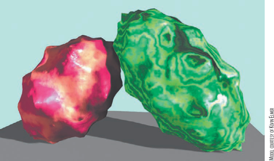
The Marble texture creates a stonelike pattern that includes virtual mineral veins. The Marble texture isn't designed to match a specific marble type, nor is the texture capable of replicating a realistic marble by itself. However, if the Marble texture is combined with other 2D and 3D textures, it becomes more convincing. For example, in Figure 5.10 a Marble texture is mapped to the Color of a Blinn material, which in turn is assigned to a cube. When the marble is used by itself, it betrays its procedural origin. When Leather, Noise, Fractal, and Cloud textures are mapped to the Color Gain, Color Offset, Vein Color, and Filler Color attributes of the Marble texture as well as the Bump Mapping attribute of the Blinn, the results become more complex. This technique of combining procedural textures makes any single procedural texture more believable.
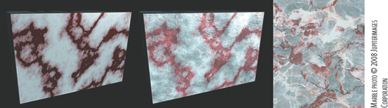
Figure 5.10. (Left) Marble texture. (Center) Marble texture with other procedural textures mapped to various attributes. (Right) Reference photo of real marble. This scene is included on the CD as marble.ma.
As for attributes, Filler Color sets the color of the stone's bulk. Vein Color sets the color of the thin veins. Vein Width sets the width of the veins. If the value is high, the veins become large spots. Diffusion controls the color mixture of the stone. Low values produce a high level of contrast between the Filler Color and Vein Color. High values allow the Vein Color to spread and mix into the Filler Color. Contrast increases or decreases the amount of contrast set by Diffusion. A Contrast value of 1 is equal to a Diffusion value of 0. Amplitude controls the complexity of the veins. Higher values create thinner veins with more kinks. You can raise the Amplitude value above the default maximum of 1.5. Ratio controls the ratio of low- to high-frequency noise. This attribute is similar to the Ratio attribute used by the Noise, Volume Noise, Fractal, and Solid Fractal textures. If the Marble texture's Ratio is raised above 0.9, however, detail is removed. The Depth and Ripples fields, which represent the Depth Min, Depth Max, Ripples X, Ripples Y, and Ripples Z attributes, function in the same manner as those belonging to the Cloud and Solid Fractal textures (see the previous section).
The Wood texture replicates the rings found in a cross-section of a tree trunk or a branch. The Wood texture is not well suited for realistic wood. However, the texture can create convincing painted or stained wood when applied as a low-intensity bump map. For example, in Figure 5.11 a Wood texture is mapped to the Bump Mapping attribute of a Blinn material, which in turn is assigned to a flattened polygon cube.
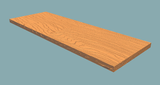
Figure 5.11. A Wood texture applied to a cube as a bump map. This scene is included on the CD as wood.ma.
On a more technical level, Vein Color establishes the color of the rings. Filler Color establishes the color of the wood between rings. Vein Spread determines how far the Vein Color will bleed into the Filler Color. A Vein Spread value of 0 will remove the Vein Color from the texture (with the exception of extremely thin ring lines). Layer Size "zooms" in and out of the pattern. Higher values create fewer rings. Randomness varies the width of each ring. When raised, Age adds more rings. Grain Color and Grain Contrast control the color and intensity of "grains" within the wood. These appear as tiny dots throughout the wood. Grain Spacing controls the distance between individual grain dots. Center sets where the circular heart of the wood is in the U and V directions.
The patterns created by the wood rings are controlled by a set of attributes in the Noise Attributes section of the Wood texture's Attribute Editor tab. Amplitude X sets the strength of noise function in the X direction. Amplitude Y does the same for the Y direction. When the 3D Placement box is at its default position, X direction corresponds with the world X axis and Y direction corresponds with the Y axis. The Ratio, Depth Min, Depth Max, Ripples X, Ripples Y, and Ripples Z attributes are identical to those of the Solid Fractal, Cloud, and Marble textures.
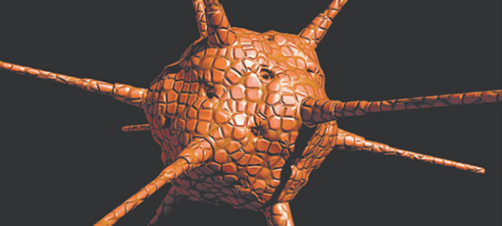
Although the Leather texture is not designed to create realistic animal hide, it can create interesting organic and cellular patterns (see Figure 5.12). Cell Color sets the color of the circular cells. Crease Color sets the color found between the cells. Cell Size determines the size of individual cells. Density determines how closely the cells are packed together. High values create less empty space between the cells and thus less color provided by Crease Color. Spottyness randomly kills off cells. High values create larger areas colored by the Crease Color. Randomness varies the pattern of cells. Low values make the distance between cells and the cell size more consistent. Threshold controls the intensity of the cell growth. High values increase the intensity of the Cell Color.
The Snow texture places a virtual snow on the areas of a surface that point toward the positive Y axis and do not possess too great a slope. The Snow texture works in conjunction with bump and displacement maps. For example, in Figure 5.13 a Fractal texture is used as a displacement map on a primitive plane. The Snow texture is mapped to the Color attribute of the Blinn connected to the displacement. As a result, all the parts of the surface that point upward are colored white. (For more information on bump and displacement mapping, see Chapter 9.)
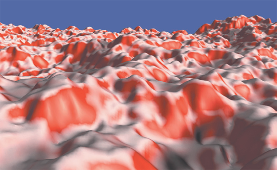
Figure 5.13. A Snow texture colors the peaks of a displaced plane. This scene is included on the CD as snow_displace.ma.
You can adjust the Snow texture to emulate fallen dust, dirt, or other debris. For example, in Figure 5.14 a Snow texture is mapped to the Color attribute of a Blinn, which is assigned to a plate and bowl. A Mountain texture is mapped to the Snow Color attribute of the Snow texture, producing white bits of debris instead of solid snow. The Threshold attribute of the Snow texture is set to 0.75, causing the debris to appear only on surface faces whose normals lie roughly between 0 and 22 degrees off the Y axis.
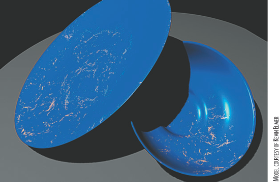
Figure 5.14. A Snow texture creates a debris-like effect over a pair of dishes. This scene is included on the CD as dish_debris.ma.
As for the Snow texture attributes, Snow Color sets the color of the virtual snow. Surface Color sets the color of the surface where the snow does not stick. (In the case of Figure 5.14, Surface Color is set to blue.) You can map this attribute with another texture for more realism. Whether or not snow sticks to a surface face is determined by the Threshold attribute. A value of 0.5 allows the snow to stick to any surface point whose surface normal lies roughly between 0 and 45 degrees off the positive Y axis. A value of 0 allows the snow to stick to any surface point whose surface normal lies roughly between 0 and 90 degrees off the positive Y axis. For example, a value of 0 would cause the snow to appear on the top half of a sphere. Depth Decay controls the transition from snow to lack of snow. High values make the transition fairly hard, and low values make the transition tapered and soft. A Depth Decay value of 0 removes the snow completely. Thickness determines the thickness of the virtual snow. High values make the snow more opaque.
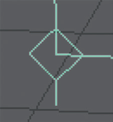
The positive Y axis used by the Snow texture is defined by the Snow texture's 3D Placement box, and not the world axis. If the box is left at its default position, the positive Y axis runs "up" in world space. However, if the box is rotated, the positive Y axis used by the Snow texture changes. When viewing the 3D Placement box, remember that the Y axis runs in the same direction as the small "tail" on the corner diamond icon (see Figure 5.2 earlier in this chapter and Figure 5.29 in the section "Placing Placement Boxes and Projection Icons").
Granular textures employ noise as grains or dots. These include Rock and Granite textures.
The Rock texture is similar to the Mountain texture in that it creates a hard-edged pattern (see Figure 5.15).
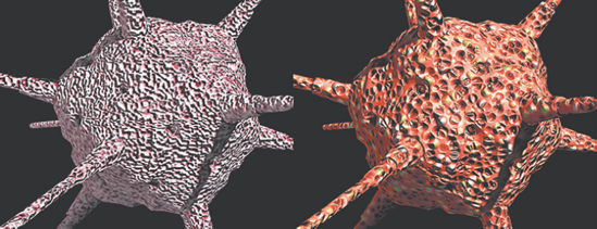
Figure 5.15. (Left) Default Rock texture applied as color and bump. (Right) Default Granite texture applied as color and bump.
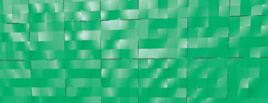
Mix Ratio sets the ratio of Color 1 to Color 2. If the Mix Ratio value is below 0.5, Color 2 becomes the grain color. If the Mix Ratio value is above 0.5, Color 1 becomes the grain color. Grain Size controls the size of the individual grains. Diffusion controls the hardness of the grain edges. Higher values blur the grains. If you increase the Grain Size and Diffusion values, you can create a stylized tile (see Figure 5.16).
The Granite texture is similar to the Leather texture in that it creates a series of colored, semicircular cells. At the same time, you can adjust the Granite texture to produce abstract patterns (see Figure 5.17).

Figure 5.17. The Granite texture is adjusted to produce an abstract pattern. This scene is included on the CD as granite_pattern.ma.
On a technical level, the texture combines three sets of cells, the color of which is determined by Color 1, Color 2, and Color 3. Cell Size determines the size of individual cells. Filler Color determines the color of the space between cells. Density controls the intensity of the cell color. High Density values reduce the amount of empty space between cells and therefore decrease the amount of Filler Color visible. Mix Ratio controls the visible ratio of the three cell colors. A value of 0 prevents the use of Color 2 and Color 3 cells. Values between 0.001 and 0.5 create a relatively equal mix of all three cell colors. Values closer to 1 favor Color 1 and Color 3. Spottyness reduces the cell density. Randomness controls the regularity of the cells. A value of 0 will align the cells in a grid. Higher values make the cells more chaotic. Threshold determines the amount of contrast between cells. Lower values reduce the contrast. Creases, when checked, inserts honeycomb-style division lines between the cells, making their shapes more irregular.
Abstract textures are not intended to replicate any real-world object. Nevertheless, they offer an interesting alternative to other textures. Stucco and Crater textures fall into this category.
The Stucco texture mixes two colors, Channel 1 and Channel 2. The Shaker attribute determines the ratio of the two colors. A high value biases Channel 1. A low value biases Channel 2.
Two Stucco attributes, Normal Depth and Normal Melt, will not function unless the Out Normal attribute of the texture is connected to the Normal Camera attribute of a material. Since this requires a custom connection, the following steps are recommended:
Create a new scene. Create a primitive object. Open the Hypershade window. MMB-drag a Blinn material into the work area. Assign the Blinn to the primitive.
MMB-drag a Stucco texture into the work area and drop it on top of the Blinn. The Connect Input Of menu opens. Choose Color from the menu. A connection line appears between the Stucco and Blinn icons. Note that the Stucco icon is named stucco1 and the Blinn icon is named blinn1.
MMB-drag the stucco1 icon on top of the blinn1 icon a second time. The Connect Input Of menu opens. Choose Other from the menu. The Connection Editor window opens.
In the left column, click Out Normal so that it becomes italicized and highlighted. Out Normal is at the very end of the list. In the right column, click Normal Camera so that it becomes italicized and highlighted. Close the Connection Editor. This connection has the effect of turning the Stucco texture into a bump map without the need for a Bump 2d or Bump 3d utility. In fact, the Bump Mapping attribute of blinn1 lists stucco1 as its connection. Close the Hypershade and render a test frame.
The Normal Depth attribute controls the depth of the bump. The Normal Melt attribute controls the smoothness of the bump. Low Normal Melt values create a rough bump with small detail, and high values create a smooth bump with large features. For information on standard bump mapping, see Chapter 9.
The Crater texture functions in a manner similar to the Stucco texture but adds extra attributes. The Crater texture mixes three colors defined by Channel 1, Channel 2, and Channel 3. The Shaker attribute controls the mixture. Shaker values below 0.1 favor Channel 1. Values from 0.1 to 0.5 favor Channel 1 and Channel 2. Values above 0.5 mix all three colors. When the value is raised above 2, the detail is reduced in scale and Channel 3 is favored. Melt controls the smoothness of the resulting pattern. Low values introduce a greater number of kinks into the threads of color. Balance controls the ratio of the three colors. As the Balance value gets higher, a greater portion of the Channel 2 color is added to the mixture. Frequency controls the scale of detail created by the color mix. High values create a finer, more convoluted pattern. Frequency is similar to the Frequency Ratio attribute of the Noise, Volume Noise, Fractal, and Solid Fractal textures.
The Out Normal attribute of the Crater texture must be connected to the Normal Camera attribute of a material for the Norm Depth, Norm Melt, Norm Balance, and Norm Frequency attributes to work. Norm Depth controls the strength of the resulting bump and is identical to the Normal Depth attribute of the Stucco texture. Norm Melt controls the smoothness of the bump and is identical to the Normal Melt attribute of the Stucco texture. Norm Balance controls the ratio between high and low points on the resulting bump. High values reduce the number of deep pits created by the bump mapping process. Norm Frequency controls the noise frequency used to generate the bump. High values create finer bump detail and introduce a greater variation between high and low points.
Although the default Crater and Stucco textures are quite vivid and match few surfaces in the real world, you can easily adjust their attributes to create a more complex result (see Figure 5.18).
Environment textures, found in the Env Textures section of the Create Maya Nodes menu in the Hypershade window, are designed to surround an object or enclose an entire scene. Environment textures require a unique rendering process. In the process, a reflection vector is derived from the camera eye vector and the surface normal of a rendered surface point (see Figure 5.19). (The angle of reflection is equal to the angle of incidence created by the camera eye vector.) Where the reflection vector strikes a placement sphere (or cube), the pixels of the texture mapped to the sphere are noted. The noted pixels are consequently used in the color calculation of the surface point. Environment textures were developed as an inexpensive way to simulate reflections.
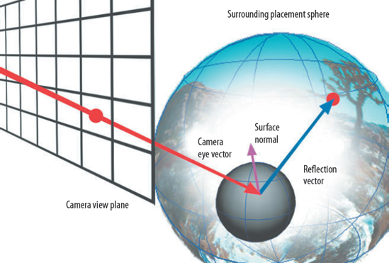
With Maya, you can successfully simulate reflections by mapping an environment texture to the Reflected Color attribute of a material. For example, in Figure 5.20 the materials assigned to a polygon car's glass, chrome, and paint have an Env Sphere texture mapped to their Reflected Color. A bitmap photo of a desert landscape is mapped to the Env Sphere's Image. As a result, a simulated reflection appears in appropriate places. Environment textures are not limited to the Reflected Color attribute, however. Any attribute is fair game. For example, an environment texture mapped to a material's Color applies the color of the Image bitmap through the camera eye vector and reflection vector process.
When you MMB-drag an environment texture into the Hypershade work area or choose it through the Create Render Node window, a 3D Placement utility is automatically connected to the texture node. This utility creates the placement sphere or cube that appears in the workspace view. Each of the five environment texture types creates a unique placement sphere or cube with specialized attributes. Although the 3D Placement utility node created for an environment texture looks similar to the 3D Placement utility node created for a 3D texture, the utilities are not identical. The 3D Placement used for a 3D texture defines the volume in which a surface point is plotted in the X, Y, and Z directions to determine a color. The 3D Placement used for an environment texture employs camera eye and reflection vectors.
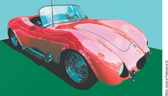
Figure 5.20. A car's reflections are provided by an Env Sphere texture. A simplified version of the scene is included on the CD as car_env_sphere.ma.
The Env Sphere texture simulates an environment by applying a map to the inner surface of an infinite sphere. You can map any texture to the Env Sphere's Image attribute. The placement icon created for the Env Sphere texture is drawn as a full circle and a half circle enclosed by two planes (see Figure 5.21). The translation and scale of the placement icon does not affect the application of the Env Sphere texture. However, the rotation of the icon will change the texture placement. The Env Sphere texture carries two unique attributes: Shear UV and Flip. Shear UV twists the mapped texture in the U and V directions (producing a barber pole effect). Flip swaps the U direction with the V direction, thus turning the mapped texture 90 degrees. Since the Env Sphere texture is based on a spherical placement, the mapped texture is pinched at the top and bottom pole.
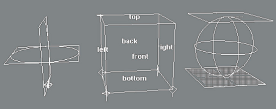
Figure 5.21. (Left) Env Sphere placement icon. (Middle) Env Cube placement icon. (Right) Env Chrome placement icon.
The Env Cube texture maps six textures to the six sides of a cube placement icon (see Figure 5.21). The scale and translation of the icon affects the application of the texture unless the Env Cube's Infinite Size attribute is checked. In either situation, the rotation of the icon changes the texture placement. The six attributes to which you can map six textures are intuitively named Right, Left, Top, Bottom, Front, and Back. The Env Cube texture is ideal for simulating an interior room.
The Env Chrome texture creates stylized chrome with a procedural ground plane and sky. The placement icon is differentiated by a top and bottom plane (see Figure 5.21). Env Chrome has an extremely long list of attributes. Nevertheless, to make the texture more realistic, I suggest the following guidelines:
Turn off the light boxes in the virtual sky by reducing Light Width and Light Depth to 0.
Turn off the dark grid on the virtual floor by reducing the Grid Width and Grid Depth to 0.
Map more realistic textures to Sky Color, Zenith Color, Horizon Color, and Floor Color. Use the same texture for Sky Color and Zenith Color as the two attributes determine the color of the virtual sky. Use the same texture for Horizon Color and Floor Color as the two attributes determine the color of the virtual ground plane.
Once you turn off the virtual light boxes and grid, you can use the Env Chrome texture to create a simulated reflection with a distinct ground plane and sky (see Figure 5.22).
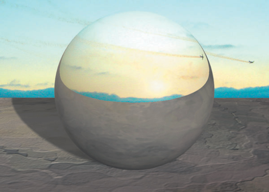
Figure 5.22. An Env Chrome texture is mapped to the color of a Blinn material, creating a simulated reflection on the surface of the sphere. This scene is included on the CD as chrome_custom.ma.
The Env Sky texture creates a procedural ground and sky, complete with a virtual sun. The placement icon is a half sphere attached to a plane. The attribute list for the Env Sky texture is as long as the Env Chrome texture. Fortunately, the attributes are intuitively named and fairly straightforward.
The Env Ball texture is designed for High Dynamic Range Image (HDRI) rendering techniques. In this case, special "light probe" images are prepared by photographing a highly reflective chrome ball in order to capture specific reflection information. For a demonstration using the Env Ball texture, see Chapter 13.
You can apply any 2D texture in three ways: Normal, As Projection, and As Stencil. The Normal method maps the texture directly to the surface with tiling controlled by the 2D Placement utility, which is connected automatically. The As Stencil method creates a shading network with a Stencil utility (see Chapter 8). The As Projection method creates a Projection utility in addition to a 3D Placement utility and a 2D Placement utility. You can check one of these three methods in the 2D Textures section of the Create Maya Nodes menu or in the Create Render Node window.
By default, when As Projection is checked and a texture selected, the Out Color attribute of the texture is connected to the Image attribute of the Projection utility. The Projection utility defines the style and coverage of the projection. The 3D Placement utility, in this scenario, stores the transform information of the Projection utility and provides the interactive projection icon. During a render, a projection ray is shot out from each pixel of the projected texture in a direction defined by the 3D Placement utility. If a projection ray strikes a surface, the pixel of the ray is noted and thereafter used in the color calculation of the struck surface point. To relate the 3D Placement utility to the Projection utility, the World Inverse Matrix attribute of the 3D Placement utility is connected to the Placement Matrix attribute of the Projection utility. (For more information on Maya matrices, see Chapter 7.)
By default, the Projection utility creates a Planar projection. The utility provides a total of nine projection styles. You can switch between these styles by changing the Proj Type attribute in the Projection utility's Attribute Editor tab. The projection styles follow:
- Off
Disables the projection. The texture connected to the Projection utility is ignored.
- Planar
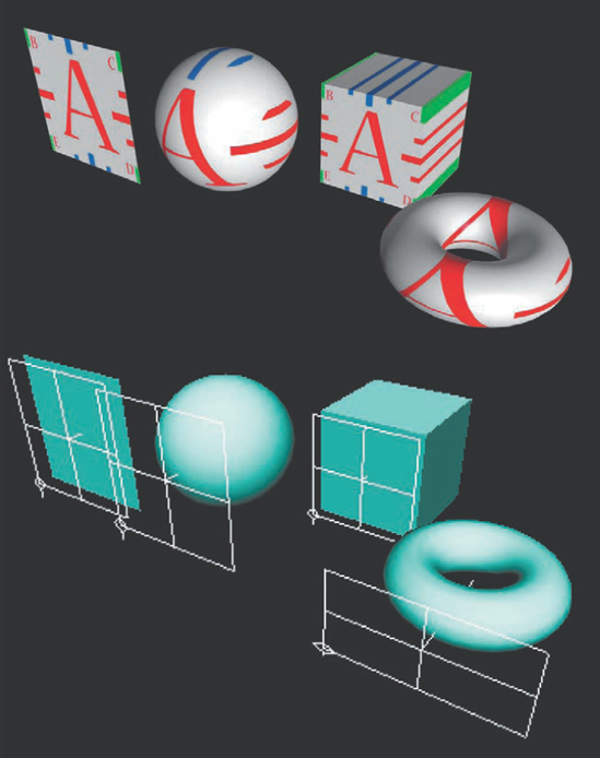
Places the texture on a projection plane. Its main disadvantage is its inability to match complex shapes. For example, in Figure 5.23 a Planar projection appears correct on a plane but streaks through a cube, sphere, and torus.
- Spherical
Places the texture inside a projection sphere. By default, the sphere is incomplete and covers only 180 degrees along the U direction and 90 degrees along the V direction. This creates a projection shape similar to a piece of paper pressed against one side of a ball. Whatever section of the assigned surface is not covered by the projection receives a repeated portion of the texture. You can create complete coverage of the projection sphere by raising the Projection's U Angle attribute to 360 and V Angle attribute to 180. Regardless of the U Angle and V Angle values, "pinched poles" will appear. That is, the upper edge of the texture is pinched into a single point, as is the lower. For example, in Figure 5.24 a Checker texture is mapped to a Surface Shader material as a Spherical projection. The top and bottom portion of the Checker is collapsed at the poles. A similar problem occurs with a NURBS sphere; even though all NURBS surfaces have four edges, two of the edges are collapsed into single points at the sphere's top and bottom pole.
Note
Although always visible, a Projection utility's V Angle attribute is functional only for a Spherical projection type. U Angle is functional only for Spherical and Cylindrical projections.
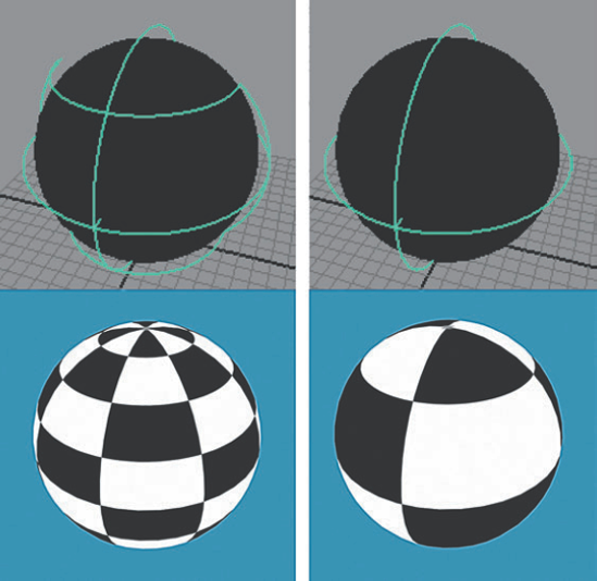
Figure 5.24. (Left) A Spherical projection with default settings is applied to a sphere. (Right) The Spherical projection's U Angle is set to 360 and its V Angle is set to 180. This scene is included on the CD as proj_spherical.ma.
- Ball
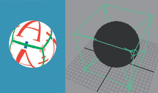
Places the texture inside a projection sphere. The projection pinches the texture at only one pole. A real-world equivalent is a blanket draped over a ball with the blanket's four corners twisted together at one spot. The pole is indicated by the diamond-shaped UV origin symbol on the projection icon (see Figure 5.25).
- Cylindrical
Places the texture inside a cylinder. The left and right edges of the texture will meet if the projection's U Angle is set to 360 degrees. The Cylindrical type creates two pinched poles at the top and bottom of the projection (see Figure 5.26).
- Cubic
Places a texture onto the six faces of a cube (see Figure 5.27).
- Concentric
Randomly selects vertical slices from the texture and projects them in a concentric pattern.
- TriPlanar
Projects the texture along three planes based on the surface normal of the object that is affected.
- Perspective
Projects the texture from the view of a camera (see Figure 5.28). For this to work, a camera must be selected from a drop-down list provided by the Link To Camera attribute (found in the Camera Projection Attributes section of the Projection utility's Attribute Editor tab). The projection icon will take the form of a camera frustum but will not be aligned to the chosen camera in 3D space. The frustum can be "snapped" to the camera, however, by connecting the Translate, Scale, and Rotate attributes of the camera's transform node to the same attributes of the 3D Placement node connected to the Projection utility node. (For more information on custom connections, see Chapter 6.)


The translation, scale, and rotation of a 3D Placement utility's placement box or projection icon affect the application of the texture mapped to it. For 3D textures, I suggest the following tips for placing the placement box:
If a surface is already assigned to the material to which the 3D Placement utility belongs, click the Fit To Group BBox button in the 3D Texture Placement Attributes section of the 3D Placement utility's Attribute Editor tab. This snaps the placement box to the bounding box of the surface.
If you need to translate, scale, or rotate the placement box, select the place3dTexture icon in the Hypershade window. You can also click the Interactive Placement button found in the 3D Placement utility's Attribute Editor tab. The Interactive Placement button selects the placement box and displays an interactive translate, rotate, and scale handle.
Unfortunately, the 3D texture icons, as they appear in the Hypershade window, are not accurate representations of the way in which the texture will render. This remains true if the placement box is scaled to fit the assigned surface. Trial and error renders provide the best fine-tuning method in this situation.
For 2D textures mapped with the As Projection option, the following tips are suggested for placing the 3D Placement utility's projection icon:
The Fit To Group BBox button found in the 3D Placement utility's Attribute Editor tab is identical to the Fit To BBox button found in the Projection utility's Attribute Editor tab. You can use either button to snap the projection icon to the assigned object or assigned group's bounding box.
If you need to translate, scale, or rotate the projection icon, select the place3dTexture icon in the Hypershade window. You can also click the Interactive Placement button found in the Projection or 3D Placement utility's Attribute Editor tab. The Interactive Placement button selects the projection icon and displays an interactive translate, rotate, and scale handle.
The projection icon created for projected 2D textures indicates the employed UV orientation. For example, a Planar projection icon features a diamond-shaped symbol at one corner (see Figure 5.29). This represents the 0, 0 origin in UV texture space. (For more information on UV texture space, see Chapter 9.) Using the origin symbol as a reference, you can orient the icon and predict the resulting render. For example, if a Planar projection icon is viewed from a front workspace view and the origin symbol is at the bottom-left corner, V runs down to up and U runs left to right, matching a texture's icon in the Hypershade window.
Spherical, Cylindrical, Ball, TriPlanar, and Cubic projection icons also carry an origin symbol. For Ball projections, the diamond shape represents the point where all four corners of the texture converge. TriPlanar projections carry three origin symbols, one at the corner of each plane. Each plane is identical to a Planar projection. Cubic projections carry six symbols, although three of them overlap at one corner. Concentric projections carry no symbols since standard UV interpretation does not apply.
For each and every example in this section, animation of the assigned surface can adversely affect the projection. If either the surface or the projection icon is moved, the surface picks up a different portion of the texture. If the surface is larger than the projection icon or is not aligned to the icon, it receives a repeated portion of the texture. To avoid this problem, you can parent the 3D Placement utility to the surface. However, this will not prevent errors when a surface deforms. Fortunately, the Convert To File Texture tool is available.
The Convert To File Texture tool allows you to convert projected 2D textures, as well as 2D and 3D procedural textures, into permanent bitmaps. To apply the tool, follow these steps:
Select a material that has a projected or procedural texture assigned to one or more of its attributes. Shift+select the surface to which the material is assigned.
Choose Edit > Convert To File Texture (Maya Software) >

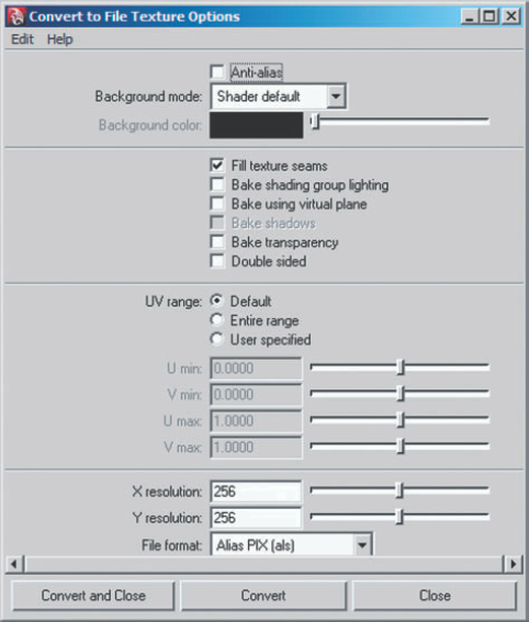
The X Resolution and Y Resolution attributes determine the size of each bitmap written out. Choose appropriate sizes and specify a File Format value. Then click the Convert And Close button.
For each projected 2D texture, procedural 2D texture, and procedural 3D texture mapped to the material, a bitmap is written to the following location with the following name:
project_directory/texture_name-surface_name.formatAt the same time, the original material is duplicated with the original shading network structure. In place of the projected and procedural textures, however, File textures are provided with the new bitmaps preloaded. The new material is automatically assigned to the surface. When compared side by side, the converted bitmap surface is virtually identical to the original (see Figure 5.31). Once the converted bitmaps are applied to the surface through the duplicated material, you can delete the original material. Thereafter, you can animate or deform the surface; the textures will not slide.
Note
Oddly enough, the Convert To File Texture tool also converts all nonprocedural bitmaps. This offers the advantage of locking in any custom UV settings. In addition, any bitmap mapped to a single channel attribute, such as Transparency or Diffuse, is converted to grayscale. The original bitmaps are not harmed.
Note
The Convert To File Texture tool will not work if the surface is assigned to the default Lambert material or if the surface is connected to more than one shading group. In general, the default Lambert material should not be used in the texturing process. You can delete connections to unneeded shading groups in the Hypershade window.
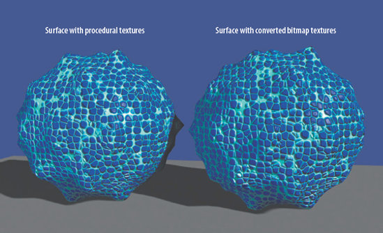
Figure 5.31. Procedurally mapped surface compared to surface with converted bitmaps. This scene is included on the CD as convert.ma.
The Convert To File Texture tool carries additional attributes for fine-tuning. Anti-Alias, if checked, anti-aliases the bitmap. Background Mode controls the background color used in the conversion. Fill Texture Seams, when checked, extends the color of any UV shell past the edge of the shell boundary; this prevents black lines from forming at the boundaries when the surface is rendered. Bake Shading Group Lighting, Bake Shadows, and Bake Transparency, when checked, add their namesake elements to the converted bitmap. Double Sided must be checked for Bake Shadows to function correctly. UV Range allows the custom selection of a non-0-to-1 range. (It is also possible to bake lighting information through the Transfer Maps window, which is discussed in Chapter 13.)
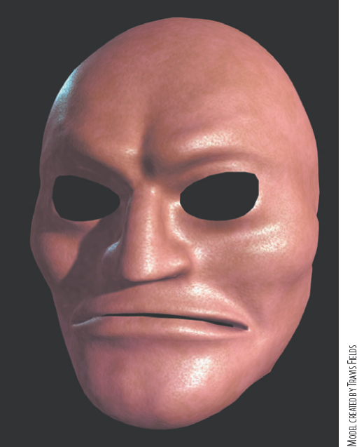
In this tutorial, you will texture a character's head using nothing more than 2D and 3D procedural textures (see Figure 5.32). Although custom bitmaps generally create the highest level of realism, the proper use of procedural textures can save a significant amount of time on any production.
Note
Open
head.mafrom the Chapter 5 scene folder on the CD. This file contains a stylized polygon head.Open the Hypershade window. MMB-drag a new Blinn material into the work area. Assign the Blinn to the head. Open the Blinn's Attribute Editor tab. Change the Color attribute to a flesh color of your choice. Change the Ambient Color to a dark red. This will give the surface a subtle, skinlike glow in the shadows. The Ambient Color slider should not be more than 1/8 of the slider length from the left side. If the Ambient Color is too strong, the surface will look washed out and flat.
To properly judge the results, create several lights. Follow either the 2- or 3-point lighting techniques discussed in Chapter 1. Render a series of tests until the lighting is satisfactory.
Open the Blinn's Attribute Editor tab. Click the Specular Color checkered Map button and choose a Fractal texture from the Create Render Node window. Double-click the place2dTexture1 icon in the work area, which opens its Attribute Editor tab. Set Repeat UV to 15, 15 and check Stagger. This reduces and randomizes the scale of the fractal pattern so that it can emulate pores.
Open the Blinn's Attribute Editor tab. Adjust the Eccentricity and Specular Roll Off attributes. Correct values depending on the lighting of the scene. The goal is to create a strong specular highlight without losing the detail provided by the Fractal texture. Be careful not to raise the Eccentricity value too high; this will spread out the highlight and make the skin look dull.
In the work area, double-click the Fractal icon (named fractal1), which opens its Attribute Editor tab. Reduce the Amplitude and raise the Threshold slightly. This reduces the amount of contrast in the fractal pattern and makes its effect subtler. Tint the Color Gain attribute a pale blue. This inserts a color other than red into the material and helps make the skin color more varied.
Open the Blinn's Attribute Editor tab. Click the Bump Mapping checkered Map button. Choose a Granite texture from the Create Render Node window. In the work area, double-click the bump3d1 icon, which opens its Attribute Editor tab. Change Bump Depth to 0.005. In a workspace view, select the 3D Placement utility's placement box and scale it down to 0.5, 0.5, 0.5 in X, Y, Z. Render a test. The Granite texture provides a subtle bumpiness/fuzziness to the parts of the skin that do not have specular highlights.
Return to the Blinn's Attribute Editor tab. Click the Incandescence checkered Map button and choose a Solid Fractal texture from the Create Render Node window. In the work area, double-click the Solid Fractal icon (named solidFractal1), which opens its Attribute Editor tab. Change the Ratio value to 1 and the Frequency Ratio value to 4. Change Color Gain to a dark purple. Render a test frame. The Solid Fractal texture introduces variation within the basic skin color. If the result is too bright or the color is not quite right, adjust the Color Gain and render additional tests.
The skin material is complete! If you decide to apply this material to a character that moves or deforms, you can use the Convert To File Texture tool to change the 3D procedural textures into bitmaps. If you get stuck with this tutorial, a finished version is included as head_finished.ma in the Chapter 5 scene folder on the CD.