Creating custom shading networks is a powerful way to texture and render with Maya. You can connect hundreds of material, texture, geometry, light, and camera attributes through the Hypershade window for unique results. In addition, you can apply specialized color utilities that can customize the hue, saturation, value, gamma, and contrast of any input and output.
Chapter Contents
A quick review of the Hypershade window
Multiple approaches for creating connections
Tips for keeping the Hypershade organized
Practical applications of each color utility
The Hypershade window is the heir to the Multilister domain. Although the Multilister window is a legacy tool from PowerAnimator, the Hypershade was created specifically for Maya. Everything that can be done in the Multilister can be done in the Hypershade, but not vice versa. You can access the Hypershade by choosing Window > Rendering Editors > Hypershade. You can access the Multilister by choosing Window > Rendering Editors >Multilister.
The Hypershade window allows the connection of various Maya nodes. Technically speaking, a node is a construct that holds specific information plus any actions associated with that information. A node might be a curve, surface, material, texture, light, camera, joint, IK handle, and so on. Any box that appears in the Hypergraph or Hypershade window is a node. (For a differentiation between transform and shape nodes, see Chapter 7.) A node's information is organized into specific attributes. If an attribute can be animated, it is called a channel (and appears in the Channel Box). For example, the Scale X of a sphere is a channel.
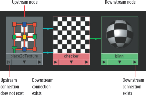
You can connect attributes in an almost endless fashion. A series of connected nodes is a node network. If the network is designed for rendering, it's called a shading network. Any node connected to any other node is considered upstream or downstream. An upstream node is a node that outputs information. A downstream node is a node that receives or inputs information. The node icons themselves will show if an upstream or downstream connection exists. If the bottom-left arrow is solid, the node is downstream of another node. If the bottom-right arrow is solid, the node is upstream of another node. If either arrow is hollow, a connection does not exist in the direction in which the hollow arrow points (see Figure 6.1).
You can create new nodes at any time by clicking a node icon in the Create Maya Nodes menu of the Hypershade window. You can also MMB-drag nodes from the Create Maya Nodes menu into the work area. To copy individual nodes, choose Edit > Duplicate > Without Network from the Hypershade menu. To copy entire shading networks, choose Edit > Duplicate > Shading Network.
You can export shading networks. Choosing File > Export Selected Network saves the selected network, by itself, in a file with the .mb or .ma extension. You can then bring networks back into the Maya scene by choosing File > Import from the Hypershade menu.
To assign materials, MMB-drag them on top of geometry in a workspace view. Alternatively, you can follow these steps:
Select the surface.
With the mouse over the material icon, right-click and choose Assign Material To Selection from the marking menu.
You can create custom connections through the Connection Editor (choose Window > General Editors > Connection Editor) or the Hypershade window's work area. Descriptions of various approaches follow.
The Connection Editor is divided into two sections. By default, the left side contains outputs (upstream) and the right side contains inputs (downstream). A single node can be displayed on each side. To load a selected material, texture, surface, or any other Maya node, click the Reload Left or Reload Right button.
To make a connection, simply select an attribute on the left and an attribute on the right. Once a connection is made, the names of the attributes become italicized. A number of attributes are grouped into sets of three, as represented by the plus sign (see Figure 6.2). This grouping is a type of vector. (See Chapter 8 for a discussion on vectors.) It occurs most commonly with the Color attribute, which is composed of Red, Green, and Blue channels, but it also applies to color-driven attributes such as Transparency and Incandescence. You can reveal the individual channels of any given vector attribute by clicking the plus sign.
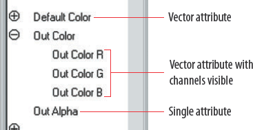
Other attributes, such as Translate or Normal Camera, represent a spatial vector with X, Y, and Z coordinates. Any vector attribute can be connected to any other vector attribute. However, a vector attribute cannot be connected to a single attribute. Nevertheless, a single attribute can be connected to any single channel of the vector (see Figure 6.3). If any attribute is dimmed out, it is nonkeyable and thereby off limits for a custom connection.

Figure 6.3. (Top) A vector attribute connected to second vector attribute. (Bottom) The single channel of a vector attribute connected to a single attribute.
Color, the most common attribute, is predictably named Color on the input (downstream) side of a node. However, it is named Out Color on the output (upstream) side. Similarly, there is Out Glow Color, Out Alpha, and Out Transparency. See the end of this section for a discussion of Out Alpha and Out Transparency.
Dragging and dropping one node on top of another using the MMB automatically opens the Connect Input Of menu (see Figure 6.4). The default attribute (usually Color) of the output (upstream) node is automatically used for the connection. The Connect Input Of menu makes no distinction between vector and single attributes. If a Connect Input Of menu selection is made that confuses the program, the Connection Editor automatically opens. The attributes listed by the Connect Input Of menu is incomplete (although they are the most common and often the most useful). To see the full list, choose Other to open the Connection Editor. Dragging and dropping one node on top of another using the MMB while pressing Shift opens the Connection Editor immediately.

Dragging and dropping one node on top of another using the MMB while pressing Ctrl instantly makes a connection. In this situation, the default attribute for both nodes is used. For instance, the default input attribute of a Blinn material is Color. The default input attribute of a bump2d node is Bump Value. If the two nodes involved in the connection are not a standard pair, Maya will not be able to make a decision. For example, dragging one texture on top of another texture with the MMB and Ctrl forces Maya to open the Connection Editor.
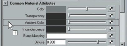
You can also MMB-drag nodes from the Hypershade window to the Attribute Editor. An outlined box appears around any valid attribute when the mouse arrow hovers over it (see Figure 6.5). Releasing the mouse button over an attribute automatically creates a connection. In this case, it's best to double-click the downstream node first to open the node's Attribute Editor tab, and then MMB-drag the upstream node without having actually selected it. Of course, clicking the standard checkered Map button on an Attribute Editor tab opens the Create Render Node window and creates a connection once a material, texture, or utility is selected.
Left mouse button (LMB)-clicking and -dragging an existing connection line creates a brand-new ghost line. If the ghost line is dropped onto another node, the Connect Input Of menu opens. If you click the original line behind the arrowhead, the ghost line starts at the input (downstream) node. If you click the original line ahead of the arrowhead, the ghost line starts at the output (upstream) node. The attribute for the node from which the ghost line extends will be the same as the original connection line (see Figure 6.6).
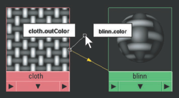
You can display the white label boxes in Figure 6.6 at any time by clicking an existing connection line. Regardless of the way nodes are arranged in the work area, the output (upstream) attribute is displayed in the white label box to the left of the mouse arrow, while the input (downstream) attribute is displayed in the white label box to the right of the mouse arrow. For example, when examining the connection in Figure 6.6, cloth.outColor appears in the left label box, while blinn.color appears in the right label box. Along these lines, output channels often carry an out prefix and therefore appear on the left, or output, label box.
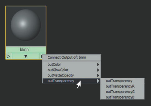
Right-clicking the bottom-right corner of a node opens the Connect Output Of menu (see Figure 6.7). Vector attributes are represented by an arrow on the right side; you can choose either the vector attribute or any single channel. Once an attribute is chosen, a connection line attaches itself to the mouse arrow. When you click another node, the Connect Input Of menu opens. Once you choose an input attribute, the connection is made. This technique works best if the camera is zoomed in fairly close to the node.
Alpha information is stored by DDS, Maya IFF, Maya16 IFF, OpenEXR, PNG, RLA, SGI, SGI16, Targa, TIFF, TIFF16, and PSD files as RGB+A and can be used by compositing programs such as Adobe After Effects and The Foundry's Nuke. Alpha represents the opacity of any given pixel in a bitmap.
You can use alpha as transparency information in Maya in two ways. The quickest method is to load the bitmap into a File texture and connect the File's Out Transparency attribute to the Transparency attribute of a material node. The second method involves the use of the PSD File texture. For example, in Figure 6.8 the transparency surrounding a frog is supplied by the alpha channel of a PSD file. In this case, alpha.psd is loaded into a PSD file texture node named psdFileTexAlpha. The outTransparency of psdFileTexAlpha is connected to the transparency of a lambert material node named LambertAlpha. The drop-down menu of psdFileTexAlpha's Alpha To Use attribute is set to Alpha 1. Last, the outColor of the psdFileTexAlpha is connected to the color of LambertAlpha.
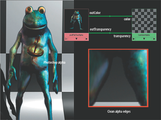
Figure 6.8. The alpha channel of a PSD file is used for transparency. This example is included on the CD as transparency.ma.
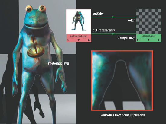
The PSD File texture can also read Photoshop layer transparency. For example, in Figure 6.9 the transparency surrounding the frog is supplied by the layer information of a second PSD file. In this case, layer.psd is loaded into a PSD file texture node named psdFileTexLayer. The outColor of psdFileTexLayer is connected to the color of a lambert material node named LambertLayer. The outTransparency of psdFileTexLayer is connected to the transparency of LambertLayer. This time, the Alpha To Use attribute of psdFileTexLayer is set to Transparency. The layer transparency technique tends to create a fine white line along the image edge, as can be seen along the frog's inner legs. This is due to Photoshop's flattening of the image as it saves (the transparency becomes premultiplied white).
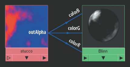
Out Alpha, on the other hand, is used most commonly as a grayscale, single-channel version of a texture. A bump2D node, for example, will connect outAlpha to its own bumpValue attribute by default. (See Chapter 9 for a discussion on bump mapping.) As an additional example, the outAlpha of a stucco texture node is connected to the colorR, colorG, and colorB of a blinn material node. The result is a grayscale version of the stucco pattern (see Figure 6.10). Out Alpha and similar single-channel attributes are sometimes referred to as scalar, whereby they possess only magnitude.
Shading networks can become complex in the Hypershade window. Hence, they are often difficult to work with unless you take steps to organize all the various nodes. A few tips for keeping the Hypershade easy to navigate follow.
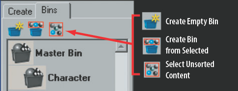
Bins are containers for nodes; the contents of only one bin can be seen in the tab area at any given time. By default, there is one Master Bin. To create new bins, click the Create Empty Bin button (see Figure 6.11). To assign a node to a bin, MMB-drag-and-drop the node from the tab area onto the bin icon. You can also select the node, RMB-click over the bin icon, and choose Add Selected from the shortcut menu. You can remove a node from a bin by choosing Remove Selected from the same shortcut menu. If necessary, a node can be assigned to multiple bins. (The entire shading network that is connected to a node will be added to any bins that the node has been assigned to.) By default, all nodes belong to the Master Bin.
Containers, on the other hand, are specialized node groupings. A container is represented by a thick, rounded edge (see Figure 6.12).
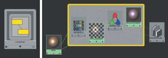
Figure 6.12. (Left) A collapsed container. (Right) An expanded container with connections to nodes not included in the container.
In terms of texturing, you can use containers as a method of organization. For example, you can select all the nodes that make up a shading network and convert them to a container with the following steps:
Select the shading network nodes in the Hypershade work area.
RMB-click one of the nodes and choose Create Container From Selected from the shortcut menu. The nodes are collapsed into a single container.
To view the original nodes, double-click the container. To hide the original nodes, double-click again.
If only a portion of a network is converted to a container, connections run from the nodes within the container to nodes outside the container. If you move the nodes that belong to a container while the container is expanded, the container automatically resizes itself. The container does not possess any of its own attributes, although you can add attributes through the Attribute Editor menu. (See Chapter 9 for information on adding attributes.) You can rename a container by opening it in the Attribute Editor tab and changing the name in the Container field. To remove selected nodes from a container, RMB-click a selected node and choose Remove From Container from the shortcut menu. You can view container nodes in the Hypergraph Hierarchy and Hypergraph Connections windows.
As for tabs, you can create, rename, or reorder custom tabs through the Hypershade window Tabs menu.
The Show Previous Graph and Show Next Graph buttons toggle through work area views. At the same time, the connection buttons offer a quick way to frame other components of a shading network (see Figure 6.13). This is particularly useful when a portion of a network has been "lost" and is no longer in view. The connection buttons also serve as a quick way to view normally hidden downstream nodes. In addition, you can find the Input Connections and Output Connections buttons can at the top of every Attribute Editor tab.
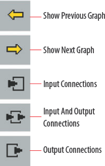
Figure 6.13. The Show Previous Graph, Show Next Graph, Input Connections, Input And Output Connections, and Output Connections buttons
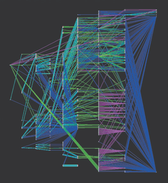
Unless a scene contains complex custom connections, you can view the majority of its node network within the Hypershade window's work area. You can even find rarely viewed nodes that represent render partitions, light linking, Timeline time, expressions, construction history, UV mappings, and Paint Effects brushes. To achieve such a view, select any node in the Hypershade work area and click the Input And Output Connections button. Select all the nodes that appear and click the button again. Repeat this process two or three times. A complex node network soon appears (see Figure 6.14). Blue lines run downstream to the renderPartition and lightLinker nodes, as well as to various utilities. Purple lines run from geometry shape nodes to shading group nodes. Cyan lines run from place2dTexture nodes to textures. Green lines run downstream to shading groups and between textures.
Occasionally, the Hypershade window will not display all the components of a custom shading network. This is particularly true when the network contains a mixture of materials, lights, and cameras. In addition, the Hypershade fails to automatically display transform nodes. Should this situation arise, the Hypergraph Connections window offers a reliable alternative. To view the entire node network of a scene within the Hypergraph, follow these steps:
Choose Window > Hypergraph: Connections. From the Hypergraph Connections window menu, choose Show > Auxiliary Nodes.
In the Auxiliary Nodes window, click-drag the mouse arrow over the nodes listed in the Node Types That Are Hidden In Editors field. With the nodes highlighted, click the Remove From List button. This guarantees that no node types are hidden in the Hypergraph Connections window. Close the Auxiliary Nodes window.
Choose Show > Auxiliary Nodes from the Hypergraph menu so that the menu item is checked. Select all the nodes that are visible. Choose Graph > Input And Output Connections from the Hypergraph menu. Select all the nodes that are visible. Choose Input And Output Connections again. Repeat the process until there is no change in the view.
Returning to the Hypershade window, right-clicking while the mouse arrow hovers over a node in the work area opens a marking menu with a Graph Network option. Choosing Graph Network reveals and frames all the upstream connections of a selected node (see section B of Figure 6.15). By default, Graph Network clears all other networks from the work area. To avoid this, right-click over an empty portion of the work area and choose (and therefore uncheck) Clear Before Graphing. A disadvantage of Graph Network is its inability to reveal nodes downstream from the selection. Right-clicking over an empty portion of the work area and choosing Graph > Rearrange Graph arranges nodes in a pattern identical to choosing Graph Network from the marking menu (although it can arrange only the nodes that are already visible).
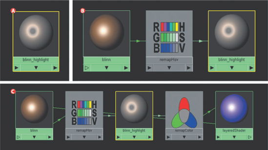
Figure 6.15. (A) A lone blinn node in the work area. (B) The work area after the application of Graph Network. (C) The work area after the alternate application of the Input And Output Connections button.
The most thorough way to organize the work area is to use the Input And Output Connections button. The resulting network is very orderly (see section C of Figure 6.15). In general, the resulting order will only break down once large swaths of the scene are viewed. The Input And Output Connections button will clear unselected shading networks from the work area. Nevertheless, the button will arrange all connected nodes if multiple shading networks are selected simultaneously.
Choosing Edit > Delete Unused Nodes from the Hypershade menu is an excellent way to thin out the Hypershade. Complex or lengthy projects often produce redundant nodes. Delete Unused Nodes deletes any node that is not assigned to a surface or is part of an assigned shading network.
Twelve utility nodes in Maya are designed to shift colors. These utilities can convert color space, remap color ranges, adjust brightness and contrast, and even read the luminance of a surface within a scene.
The Rgb To Hsv utility converts a Red/Green/Blue vector into a Hue/Saturation/Value vector. The Hsv To Rgb utility does the opposite. In Maya, Red, Green, and Blue channels have a numeric range of 0 to 1. In HSV color space, Hue corresponds to a pure color and has a range of 0 to 360. Saturation, which represents the amount of white mixed into a color, has a range of 0 to 1. Value, which represents the amount of black mixed into a color, also has a range of 0 to 1. With the Hsv To Rgb utility, inHsvR carries the hue, inHsvG carries the saturation, and inHsvB carries the value. In contrast, the Rgb To Hsv utility offers inRgbR, inRgbG, and inRgbB, which represent the standard red, green, and blue color components.
The Rgb To Hsv and Hsv To Rgb utilities allow calculations to stay in HSV color space. In addition, the Hsv To Rgb utility can serve as a color "dial." For example, in Figure 6.16 a bitmap is tinted different colors as the Timeline progresses.
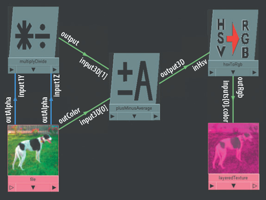
Figure 6.16. An Hsv To Rgb utility is used to create a color dial. This scene is included on the CD as hsvtorgb.ma.
To view the shading network, follow these steps:
A bitmap named greyhound.tif is loaded into a File texture. The outColor of the file node is connected to the input3D[0] of a plusMinusAverage node. The output3D of the plusMinusAverage node is connected to the inHsv of an hsvToRgb node. As a test, outRgb of the hsvToRgb node is connected to the inputs[0].color of a layeredTexture node. The output of a multiplyDivide node is connected to input3D[1] of the plusMinusAverage node. The plusMinusAverage node's Operation is set to Average. (For information on the Multiply Divide and Plus Minus Average utilities, see Chapter 8.) Last, the outAlpha of the file node is connected to input1Y and input1Z of the multiplyDivide node.
The multiplyDivide node serves as the color dial controller. The multiplyDivide node's Input1X attribute determines the outgoing hue since it is connected to inRgbR. Input1X is animated with keyframes so that the value changes from 0 to 359. This creates a complete clockwise revolution of the HSV color wheel (which is a counterclockwise spin on Maya's RGB color wheel). The plusMinusAverage node averages the hue value provided by the multiplyDivide node and the outColorR channel value of the texture. In this way, the final texture is not washed out or completely overtaken by the new hue value. The outAlpha of the file node determines the saturation of the final texture as it is connected to the input1Y of the multiplyDivide node, which in turn is connected to inRgbG of the hsvToRgb node. The outAlpha also determines the value (the amount of mixed-in black) of the final texture as it is connected to the input1Z of the multiplyDivide node, which in turn is connected to inRgbB of the hsvToRgb node.
Table 6.1 shows what happens to different color pixels of the original texture if the Input1X of the multiplyDivide node is set to 100.
Table 6.1. Colors Resulting from Different Texture Pixel Values
Texture Pixel RGB | multiplyDivide Output | plusMinusAverage Output | hsvToRgb Output |
|---|---|---|---|
0, 0, 0 | 100, 0, 0 | 50, 0, 0 | 0, 0, 0 (black) |
0.5, 0.5, 0.5 | 100, 0.5, 0.5 | 50.25, 0.5, 0.5 | 0.5, 0.459, 0.25 (brown) |
1, 0.6, 1 | 100, 0.6, 1 | 50.5, 0.6, 1 | 1, 0.905, 0.4 (light orange) |
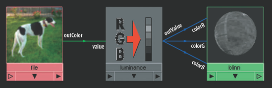
The Luminance utility converts RGB values into luminous values. In Maya, a luminous value signifies the apparent brightness of a color as seen by the human eye. The Luminance utility's Out Value attribute outputs a scalar (a single channel) version of the input. For example, in Figure 6.17 the outColor of a file texture node is connected to the value of a luminance node. The outValue of the luminance node is connected to the colorR, colorG, and colorB of a blinn material node. The result is a grayscale version of the original bitmap. The Out Value attribute varies from the common Out Alpha attribute in that it biases the green channel. Colors are not perceived equally by the human brain; hence, the Luminance utility uses the following formula:
outColor= (0.3 ×Red) + (0.59 ×Green) + (0.11 ×Blue)
The Blend Colors utility blends two colors or textures together using a third color or texture as a control. The Blend Colors formula is as follows:
outColor= (Color1×Blender) + (Color2× (1 -Blender))
If the Blender attribute is 1, Color1 is the resulting output. If Blender is 0, Color2 is the resulting output. If Blender is 0.5, a percentage of Color1 and Color2 are added. For example, in Figure 6.18 the Blend Colors utility is used to create a logo stenciled onto a wall. logo_mask.tif is loaded as a File texture. The outAlpha of the file node is connected to the blender of a blendColors node. wall.tif is brought in as a second File texture. The outColor of the second file node is connected to color1 of the blendColors node. logo_color.tif is brought in as a third File texture. The outColor of the third file node is connected to color2 of the blendColors node. The output of the blendColors node is finally connected to the color of a blinn material node. The raggedness of the logo is generated by logo_mask.tif. (For a discussion on the Stencil utility, which can provide results similar to this example, see Chapter 8.)

The Remap Color utility allows the adjustment of a color attribute through the use of interactive gradients. A gradient functions like a horizontal ramp. Technically speaking, a gradient is a graphic representation of the transition between two colors. The far-left side of a gradient represents the output color value that will be given to the lowest values of the input color. The far-right side of the gradient represents the output color value that will be given to the highest values of the input color. With the default upward slope, 0 is given 0, 0.5 is given 0.5, and 1 is given 1, and thus there is no change.
The simplest way to see the Remap Color utility functioning is to reverse the gradient slope. In Figure 6.19, the outColor of a grid texture node is connected to the color of a remapColor node. The outColor of the remapColor node is connected to the color of a lambert material node. When the slope direction is reversed on each gradient, the whites become black (RGB: 1, 1, 1 to 0, 0, 0) and the blacks become white (0, 0, 0 to 1, 1, 1).
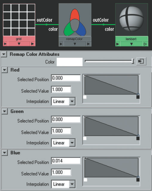
Figure 6.19. A Grid texture is inverted with a Remap Color utility. This material is included on the CD as remap_invert.ma.
In a second example, a Noise texture is used (see the top of Figure 6.20). The far left handle of the Red gradient is moved to the top. This forces the texture to carry the maximum amount of red at all points. Thus, black becomes pure red (0, 0, 0 to 1, 0, 0). White is unchanged since it already contained the maximum amount of red (1, 1, 1 to 1, 1, 1). Gray turns into a pale red (0.5, 0.5, 0.5 to 1, 0.5, 0.5).

Figure 6.20. (Top) Black is shifted to red with a Remap Color utility. This material is included on the CD as remap_red_1.ma. (Bottom) White is shifted to cyan with a Remap Color utility. This material is included on the CD as remap_red_2.ma.
In a third example (see the bottom of Figure 6.20), a Noise texture is used again. This time, the Red gradient is reversed and then given a plateau by inserting an additional handle. Any part of the Noise texture that has a red value of 0.5 or less receives the maximum amount of red. Any part of the Noise texture that has a red value greater than 0.5 receives less red, allowing the green and blue to triumph and thus produce a cyan color.
You can insert additional handles into any of the three gradients by clicking in the dark gray area. You can move any handle up/down and left/right by LMB-dragging. Any handle can be deleted by clicking its × box. You can change the transition from handle to handle by switching the gradient's Interpolation attribute from Linear to Smooth, Spline, or None.
The Remap Color utility is not limited to color attributes. For example, in Figure 6.21 the translate of a sphere transform node is connected to the color of a remapColor node. The outColor of remapColor is connected back to the transform node's rotate. The gradients on the remapColor node are set to numerous jagged peaks and valleys. As a result, the sphere automatically undergoes an erratic rotation when moved in any direction. The Remap Color utility's Input Min and Input Max are set to −10 and 10, respectively. This prevents the rotation from continuing when the sphere's translation exceeds 10 units in the X, Y, or Z direction. The Output Min and Output Max are set to −360 and 360, respectively. This forces the remapped translate values to stay between −360 and 360, which permits the sphere to rotate in any direction for a single revolution.
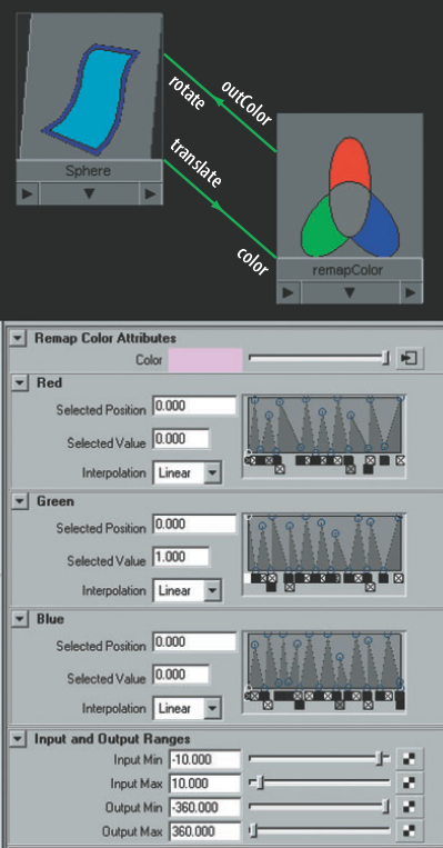
Figure 6.21. The rotation of a sphere is automatically driven, and made erratic, with a Remap Color utility. This scene is included on the CD as remap_rotate.ma. A QuickTime movie is included as remap_rotate.mov.
To view the custom shading network, follow these steps:
Open
remap_rotate.mafile from the CD. Open the Hypershade window.Switch to the Utilities tab. MMB-drag the remapColor node into the work area.
With the remapColor node selected, click the Input And Output Connections button. The network becomes visible.
Note
You can MMB-drag any node that is visible in the Hypergraph into the Hypershade work area. This includes geometry. Any node that appears in any tab of the Hypershade can be MMB-dragged into the work area as well. This includes cameras, lights, and shading groups.
The Remap Hsv utility works in the same fashion as the Remap Color utility. Instead of offering Red, Green, and Blue gradients, however, it carries Hue, Saturation, and Value gradients. By separating Hue from Value, it's possible to isolate very narrow sections of a texture or material. For example, in Figure 6.22 the specular highlight of a Blinn material is given an artificial chromatic aberration. Optically, chromatic aberration is the inability of a lens to focus various color wavelengths on the same focal plane. This artifact often appears in both traditional and digital color photography and is referred to as "purple fringing."
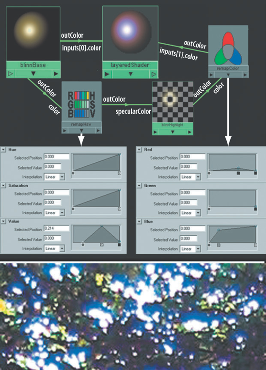
Figure 6.22. (Top) The specular highlight of a Blinn is given an artificial chromatic aberration with a Remap Hsv utility. This material is included on the CD as remap_hsv.ma. (Bottom) Chromatic aberration is visible as a "purple fringing" in a photograph of tree foliage.
To achieve the purple fringe on the highlight, the outColor of a blinn material node, named blinnBase, is connected to the color of a remapHsv node. The outColor of remapHsv is connected to the specularColor of a second blinn material node named blinnHighlight. The outColor of blinnHighlight is connected to the color of a remapColor node. The outColor of remapColor is connected to the inputs[1].color of a layeredShader material node. The outColor of blinnBase is connected to the inputs[0].color of the layeredShader node. By adjusting the remapHsv Value gradient, a narrow sliver of the blinnBase specular highlight is retrieved. This is visible on the icon of blinnHighlight (which has its Transparency attribute set to 100% white). The remapColor node tints the pulled highlight a purplish color. The layeredShader node is able to combine the isolated purplish highlight and the original blinn.
Although the Remap Value utility controls color through two gradients, its basic functionality is different from Remap Color and Remap Hsv utilities. Remap Value provides a single-channel Value gradient that can be used by itself. (See Chapter 7 for an example of the Remap Value utility used in such a way for car paint.)
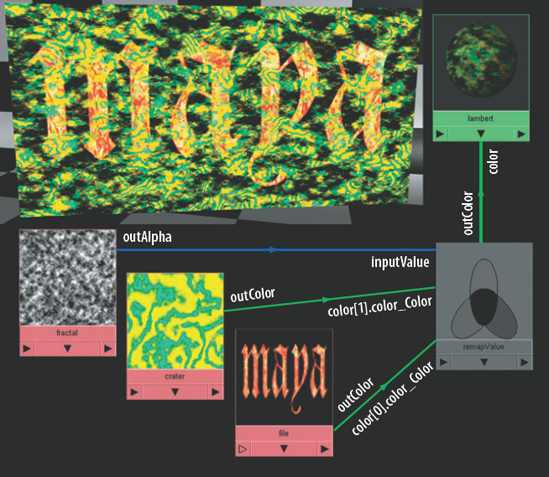
The Remap Value utility also provides a Color gradient. The Color gradient is controlled by the Input Value attribute. That is, if a texture mapped to the Input Value attribute provides the color black, the left side of the Color gradient is sampled. If a texture mapped to the Input Value attribute provides the color white, the right side of the Color gradient is sampled. Hence, the Remap Value utility supports an additional method of blending two sources together.
For example, in Figure 6.23 maya.tif is brought in as a File texture. The outColor of the file texture node is connected to color[0].color_Color of a remapValue node. This connection attaches the file node to a handle within the Color gradient. The outColor of a crater texture node is connected to color[1].color_Color of the remapValue node. This connection attaches the crater node to a second Color gradient handle. The handles are arranged so that the file node handle is at the far right of the gradient and the crater node handle is at the far left. The outAlpha of a fractal texture node is connected to inputValue of the remapValue node. Thus, the fractal node becomes a controller for the Color gradient. Black spots within the fractal cause the remapValue node to select color from the crater node. White spots within the fractal cause the remapValue node to select color from the file node. Gray spots cause the remapValue node to add the file and crater together to determine a color. The outColor of the remapValue node is finally connected to the color of a lambert material node, which in turn is assigned to a plane. In the end, the lambert color is a mixture of the crater and file based on the pattern provided by the fractal.
The Smear utility allows one texture to be distorted by another. If Smear is combined with a Ramp texture, it creates a stylized vision effect that might be appropriate for an alien, a monster, or a robot. For example, in Figure 6.24 a sequence of video images is loaded into a File texture. The Use Image Sequence attribute is checked so that the images are automatically loaded as the Timeline moves forward. The outColor of the file node is connected to the inRgb of a smear node. The outU of the smear node is connected to the offsetU of the place2dTexture node of a ramp texture node. The outV of the smear node is also connected to the offsetV of the place2dTexture node of the ramp node. The outColor of the ramp node is finally connected to the outColor of a surfaceShader material node, which is assigned to a primitive plane. The ramp has three handles: one red and two orange. The higher the values are in the video image bitmaps, the farther the smear node "pulls" the ramp down in the V direction. For instance, if a bitmap provides a pixel with RGB values 0.5, 0.5, 0.5, the ramp is pulled downward so that the top rests at the center of the ramp field. If a bitmap provides a pixel with RGB values 0.9, 0.9, 0.9, the ramp is pulled downward so that the top rests one tenth above the bottom of the ramp field. When the ramp is called upon by the surfaceShader material, every pixel of the ramp is offset in the V direction by a unique amount. Hence, the ramp appears as a colored version of the video bitmap.
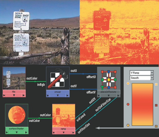
Figure 6.24. An image sequence and a Ramp texture are combined with the Smear utility. This scene is included on the CD as smear.ma. A QuickTime movie is included as smear.mov.
Internally, the Smear utility converts the input RGB to HSV. New UV coordina1es are generated by plotting values on an HSV color wheel. For another example of the Smear utility, see the tutorial at the end of this chapter.
Gamma correction is the adjustment of an image to compensate for the physical limitations of a computer monitor. With a monitor, the intensity (brightness) of a screen pixel does not linearly increase with the application of additional voltage. Because of this, uncorrected images may appear inappropriately dark or washed-out. Gamma correction solves this by applying a complementary intensity curve to the image to negate the monitor's intensity curve. Different operating systems apply gamma correction in different ways, whether through hardware or software controls. Microsoft-based systems generally operate with a gamma value set to 2.2, whereas Macintosh systems operate with a gamma value set to of 1.8. Some programs, like Adobe Photoshop, allow you to apply different gamma values to the system on the fly.
Gamma correction is applied to the image with the following standard formula:
new pixel value = image pixel value ^ (1.0 / gamma value)
Thus, if an image pixel has a value of 0.5, 0.5, 0.5 and the gamma value is set to 2.2, the new pixel value, which is sent to the screen, is roughly 0.73, 0.73, 0.73.
Maya's Gamma Correct utility also applies the standard gamma formula:
outValue=value^ (1.0 /Gamma)
In this case, the Gamma Correct utility adjusts the values of the value input and outputs the result through outValue. No other node is affected. As a rule of thumb, the higher the Gamma attribute values are, the more washed out the mid-range values become. High- and low-range values (white whites and black blacks) are affected to a lesser degree.
An interesting side effect of the Gamma Correct utility is the increase or decrease of saturation. For example, in Figure 6.25 face.tif is loaded into a File texture. The outColor of the file node is connected to the value of a gammaCorrect node. As a test, the outValue of the gammaCorrect node is connected to the inputs[0].color of a layeredTexture node. The Gamma attribute of the gammaCorrect node is set to 0.5, 0.5, 0.5. As a result, the washed-out bitmap gains a good deal of saturation. Raising the Gamma above 1 would have the opposite effect—less saturation.

Figure 6.25. A washed-out face bitmap is given extra saturation with a Gamma Correct utility. This shading network is included on the CD as gamma_correct.ma.
To view the custom shading network, follow these steps:
Open the
gamma_correct.mafile from the CD. Open the Hypershade window.Switch to the Utilities tab. MMB-drag the gammaCorrect node into the work area.
With the gammaCorrect node selected, click the Input And Output Connections button. The network becomes visible.
Note
Many Maya utilities feature vector attributes that are represented by three number fields (for example, Gamma). These fields are read left to right when representing color (red, green, blue) or position (X, Y, Z). When one of these fields is used in a custom shading network, the connection is made to a single channel of the attribute (for example, gammaX).
The Contrast utility does exactly what its name implies. The higher the Contrast attribute value of the Contrast utility, the whiter the whites and the blacker the blacks become. The lower the Contrast attribute value, the more the colors converge toward each other. The Bias attribute determines the RGB values that the colors converge to. For example, in Figure 6.26 face_2.tif is loaded into a File texture. The outColor of the file node is connected to the value of a contrast node. As a test, the outValue of the contrast node is connected to the inputs[0].color of a layeredTexture node. The Contrast attribute of the contrast node is set to 4, 4, 4. The Bias attribute is set to 0.4, 0.4, 0.4. The resulting image has extremely white whites and black blacks and few colors in the mid-ranges.

Figure 6.26. A washed-out face bitmap is given a great deal of contrast with the Contrast utility. This shading network is included on the CD as contrast.ma.
A Contrast value of 1 and a Bias value of 0.5 leaves the texture unchanged. Lowering the Contrast value reduces the contrast. Raising the Bias value darkens the texture overall.
In Maya, many sliders that include number fields can readjust themselves. For instance, a Diffuse attribute slider normally runs from 0 to 1. However, if you enter 2 into the field, the slider automatically readjusts itself to run between 0 and 4. For the Diffuse attribute, higher values result in a predictably brighter surface. Other sliders, when pushed past their default range, will not display a perceptible change. Any Maya color channel can exceed the standard bounds of 0 to 1. Although it's not possible to do this directly through the Attribute Editor, you can enter extra-high values into the fields of the Color Chooser window. To do so, follow these steps:
In the Attribute Editor tab, click the color swatch of an attribute. The Color Choose window opens.
Choose either RGB or HSV from the color space drop-down menu. If you choose RGB, enter a value into the Red, Green, or Blue field. There is no practical limit to the size of the number you enter. If you choose HSV, enter a value into the Hue, Saturation, or Value field. Although Hue and Saturation accept large numbers, the Value field is generally the most useful for custom values.
Click the Accept button to close the window.
In addition, you can create extra-high values, either intentionally or unintentionally, through custom connections. As a demonstration, the Line Color and Filler Color attributes of a grid texture node are set to 0.5, 0.5, 0.5 in RGB, creating a solid gray (see Figure 6.27). The outColor of the grid node is connected to the input1 of a multiplyDivide node (see Chapter 8 for a description). The output of the first multiplyDivide node is connected to the input1 of a second multiplyDivide node. The output of the second multiplyDivide node is connected to a blinn material node. The Input2 attribute of the first multiplyDivide node is set to 4, 4, 4. The end result, as seen in the second multiplyDivide node, is an RGB color with values of 2, 2, 2. These inappropriately high values are often referred to as super-white. From a practical standpoint, Maya simply clamps any color over 1.0 to 1.0 when rendering standard images. Even though the RGB is 2, 2, 2, it's rendered as if it's 1, 1, 1 (as seen on the blinn icon). Nevertheless, the super-white values can cause problems with custom connections if they are not taken into account. Fortunately, the Clamp utility can solve this problem (see the next section).
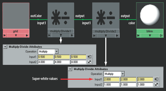
Figure 6.27. A shading network designed to test super-white values. This network is included on the CD as superwhite.ma.
To view the custom shading network, follow these steps:
Open the
superwhite.mafile from the CD. Open the Hypershade window.Switch to the Utilities tab. MMB-drag the multiplyDivide1 node into the work area.
With the multiplyDivide1node selected, click the Input And Output Connections button. The network becomes visible.
Note
Maya supports high-dynamic range (HDR) image formats, which are able to store super-white values. See Chapter 13 for details.
Note
The term super-white was coined to describe the disparity between the standard definition of video white (100 IRE units in YUV color space) and the RGB color space used by Maya and other digital-imaging programs. Basically, Maya creates whites that are 9 percent above the color range that a television can actually display. For more details on color space and monitor calibration, see Chapter 1. For a discussion of 8-bit versus 16-bit rendering, see Chapter 10.
The Clamp utility is designed to keep a value within a particular range. If a value is too low or too high, it "clamps" it. As an example, Table 6.2 shows what happens to inputR values if MinR is set to 0.3 and MaxR is set to 1.0.
Table 6.2. Clamped Output Values Resulting from Different Input Values
inputR | 0 | 0.2 | 0.8 | 1.1 | 4.5 | 9.0 |
outputR | 0.3 | 0.3 | 0.8 | 1.0 | 1.0 | 1.0 |
In this example, if the inputR value is less than 0.3, the outputR value is 0.3. If inputR is greater than 1.0, outputR is 1.0. If inputR is between 0.3 and 1.0, outputR is the same value. The Clamp utility has three inputs and three output channels (inputR, inputG, inputB, outputR, outputG, and outputB); you can connect single attributes to any of these. Otherwise, you can connect vector attributes directly to Input or Output. In a similar fashion, Min and Max, which set the clamp range, are vector attributes that carry three channels each (minR, minG, minB, maxR, maxG, and maxB). You can enter negative or positive values into the Min and Max fields.
Note
For an example of the Clamp utility used to drive a character bicep, see Section 6.1 of the Additional_Techniques.pdf file on the CD. For an example of the Clamp utility used to create disco ball glitter, see Chapter 7.
During a render, the Surface Luminance utility automatically reads the luminance of every single rendered point on the surface assigned to a material that is part of the same shading network. That is, the utility can determine the total amount of light a point on a polygon face receives and outputs a value from 0 to 1 that represents this.
As an example, in Figure 6.28, a custom crosshatch material is applied to a medallion model. The crosshatch pattern is generated by a Ramp texture and a Surface Luminance utility.
The outValue of a surfaceLuminance node is connected to the colorEntryList[0].position of a ramp texture node. The colorEntryList[n].position attribute controls the vertical position of a color handle in a ramp texture. In this case, the surfaceLuminance node drives the black color handle up and down the ramp based on how much light a surface point receives. If a surface point receives the maximum amount of light, the outValue of the surfaceLuminance node is 1, which forces the black handle up to the top of the ramp (leaving the entire ramp field white). If a surface point receives a little light, the outValue is a lower value, which allows the black handle to stay low, thus creating a mix of black and white within the ramp color field.

Figure 6.28. A crosshatch material is created with a standard Ramp texture and a Surface Luminance utility. This material is included on the CD as crosshatch.ma. A QuickTime movie is included as crosshatch.mov.
The ramp's Type attribute is set to UV Ramp; this allows the pattern to repeat on the surface vertically and horizontally. The ramp's Interpolation attribute is set to None, giving the rendered lines a hard edge. The ramp's Noise attribute is set to 0.1 and Noise Freq is set to 0.05 in order to give the lines some squiggle. The ramp node has a standard place2dTexture node with a Repeat UV set to 25, 25. Higher repeat values will produce finer lines. The place2dTexture node also has its Rotate Frame set to 45 in order to angle the pattern. Last, the outColor of the ramp node is connected to the outColor of a surfaceShader material node, which is assigned to the medallion.
In this tutorial, you will create a custom material that transforms a photo into a stylized painting (see Figure 6.29). You will use the Smear, Remap Hsv, and Contrast utilities.
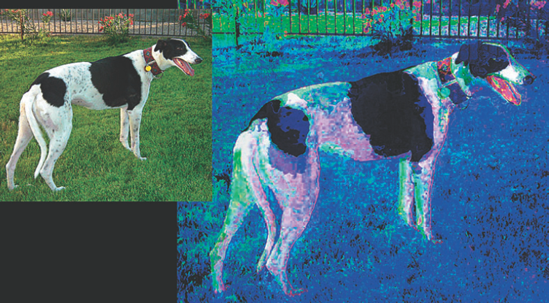
Figure 6.29. (Left) A digital photo. (Right) The same photo after the application of a custom paint material.
Create a new Maya scene. Open the Hypershade window.
MMB-drag a new Layered Texture utility (located in the Other Textures section of the Create Maya Nodes menu) into the work area.
MMB-drag two Remap Hsv utilities (located in the Color Utilities section of the Create Maya Nodes menu). Place them to the left on the layeredTexture node. Use Figure 6.30 as a reference. Rename the top remapHsv node remapHsvA. Rename the bottom remapHsv node remapHsvB.
Connect the outColor of remapHsvA to inputs[1].color of the layeredTexture node. (For a review of how to create custom connections, refer to the beginning of this chapter.)
Connect the outColor of the remapHsvB to inputs[0].color of the layeredTexture node.
Select remapHsvA and open its Attribute Editor tab. Click the Color checkered Map button and select a File texture from the Create Render Node window. A place2dTexture node is automatically created along with a file texture node. Rename this place2dTexture node place2dTextureA. Rename the file node FileA.
Select remapHsvB and open its Attribute Editor tab. Click the Color checkered Map button and select a File texture from the Create Render Node window. A second place2dTexture is automatically created along with a second file texture node. Rename the new place2dTexture node place2dTextureB. Rename the new file node FileB.
Select FileA and open its Attribute Editor tab. Click the File Browse button beside Image Name and choose
greyhound.tiffrom the Chapter 6 textures folder on the CD.Select FileB and open its Attribute Editor tab. Click the File Browse button beside Image Name and choose
greyhound.tiffrom the Chapter 6 textures folder on the CD.MMB-drag a Smear utility (located in the Color Utilities section of the Create Maya Nodes menu) into the work area. Place it to the left of place2dTextureB.
Connect the outU of the smear node to the offsetU of place2dTextureB. Connect the outV of the smear node to the offsetV of place2dTextureB.
Select the smear node and open its Attribute Editor tab. Click the In Rgb checkered Map button and choose a Fractal texture from the Create Render Node window. A new place2dTexture node is automatically created. Name this latest place2dTexture node place2dTextureC.
Select the fractal node and open its Attribute Editor tab. Change the Amplitude attribute to 0.7 and the Threshold attribute to 0.2. This will wash out the fractal pattern and reduce the contrast. If the fractal node is left with default values, the distortion created by the smear node will be extremely intense and the greyhound bitmap will no longer be recognizable. Move the Color Gain attribute slider (located in the Color Balance section) until it's barely above black. This will also reduce the intensity of the distortion. Try different positions on the Color Gain slider. Small changes will produce greatly different results.
Select place2dTextureC and open its Attribute Editor tab. Change the Repeat UV attribute to 0.6, 0.6. When the Repeat UV value is reduced, the blobs with the Fractal become larger; this, in turn, creates larger waves in the smear node's distortion. Try different Repeat UV values to see different variations of the effect.
Select remapHsvA and open its Attribute Editor tab. Change the Hue, Saturation, and Value gradients to roughly match the left side of Figure 6.31. To move points on a gradient, select the little circles and LMB-drag. To insert new points, click inside the dark gray area of each gradient. To delete a point, click the × box below it. These adjustments are shifting the hue, saturation, and value of the undistorted greyhound bitmap.
Select remapHsvB and open its Attribute Editor tab. Change the Hue, Saturation, and Value gradients to roughly match the right side of Figure 6.31. These adjustments are shifting the hue, saturation, and value of the distorted greyhound bitmap.
Select the layeredTexture node and open its Attribute Editor tab. Click the leftmost purple box. This displays the options for remapHsvB. Change the Alpha attribute to 0.5. This allows a 50–50 mix between the remapHsvA and remapHsvB nodes. (The Blend Mode attribute should be set to Over.)
MMB-drag a Contrast utility (located in the Color Utilities section of the Create Maya Nodes menu) into the work area. Place it to the right of the layeredTexture node. Connect the outColor of the layeredTexture node to the value of the contrast node.
MMB-drag a new Blinn material into the work area. Place it to the right of the contrast node. Connect the outValue of the contrast node to the color of the blinn node. Select the contrast node and open its Attribute Editor tab. Change the Contrast attribute to 1.5, 1.5, 1.5 and the Bias attribute to 0.7, 0.7, 0.5. This adjusts the contrast of the layeredTexture node. Try different numbers to see different results.
Select place2dTextureB and open its Attribute Editor tab. Change the Translate Frame attribute to 0, 0.1. This raises the FileB up a tiny amount in the V direction, which counteracts the downward pull of the smear node.
MMB-drag a Bump 2D utility (located in the General Utilities section of the Create Maya Nodes menu) into the work area. Connect outAlpha of FileB to the bumpValue of the bump2d node. Connect outNormal of the bump2d to normalCamera of the blinn node. Since outNormal is not a default attribute of a Blinn material, you will have to use the Connection Editor. Select the bump2d node and open its Attribute Editor tab. Change the Bump Depth value to 0.3. This bump mapping will give the smear distortion a sense of thickness.
The custom paint material is complete! Assign the blinn material node to a primitive NURBS plane; add a directional, point, or spot light and render out a test. It should look similar to Figure 6.29. If you get stuck, a finished version of the material is saved as
paint.main the Chapter 6 scene folder on the CD.