Sampler utilities can automate a render. They can evaluate every surface point for every frame and return unique values that other nodes can use. At the same time, you can connect cameras, lights, and geometry for unique shading networks. Along similar lines, the Studio Clear Coat plug-in utility creates surface qualities unavailable to standard materials.
Chapter Contents
Review of the Ramp Shader material and coordinate spaces
Practical applications of sampler utilities
Review of software-rendered particles
Connecting materials to nonmaterial nodes
Creating shading networks with multiple materials
The unique functionality of the Studio Clear Coat plug-in utility
The Sampler Info, Light Info, Particle Sampler, and Distance Between utilities can all be described as samplers. They sample surface points, object transforms, or particle transforms automatically throughout the duration of an animation. You can find the Sampler Info, Light Info, and Distance Between utilities in the General Utilities section of the Create Maya Nodes menu in the Hypershade window. You can find the Particle Sampler utility in the Particle Utilities section. Before I discuss the Sampler Info or Light Info utilities, however, a look at the Ramp Shader material and a review of coordinate space is warranted.
The Ramp Shader material has a Color Input attribute that has Light Angle, Facing Angle, Brightness, and Normalized Brightness options (see Figure 7.1).

Figure 7.1. (Left) The Selected Color gradient and Color Input attribute of a Ramp Shader material. (Right) The resulting material assigned to a primitive sphere lit from screen right. To see a larger version of the gradient, click the large button to the gradient's right. This scene is included on the CD as ramp_shader.ma.
The Color Input attribute allows the Ramp Shader to sample different points along the Selected Color gradient based on feedback from the environment. With Light Angle, the material compares the angle of the surface normal to the direction of the light. If the angle between the two is small, a high value is returned and the right side of the gradient is sampled. If the angle between the two is large, a small value is returned and the left side of the gradient is sampled. On a technical level, the surface normal vector and the light direction vector are put through a dot product calculation, producing the cosine of the angle between the two vectors. For a deeper discussion on vectors and vector math, see Chapter 8.
This technique is also used for the Facing Angle option, whereby the angle of the surface normal is compared to the camera direction. The Brightness option, on the other hand, calculates the luminous intensity of a surface point. If the surface receives the maximum amount of light, the right side of the gradient is sampled. If the surface receives a moderate amount of light, the middle of the gradient is sampled. The gradient runs 0 to 1 from left to right. The Light Angle, Facing Angle, and Brightness calculations are normalized to fit to that scale.
The disadvantage of the Ramp Shader is its inflexibility. Although colors can be changed on the Selected Color gradient, the Facing Angle, Light Angle, and Brightness calculations cannot be fine-tuned. Sampler Info, Light Info, and Surface Luminance utilities solve this problem by functioning as separate nodes. The Sampler Info utility replaces the Facing Angle option. The Light Info utility replaces the Light Angle option. The Surface Luminance utility, as detailed in the previous chapter, replaces the Brightness option. Although the Normalized Brightness option normalizes all the light intensities in the scene, its basic function is identical to Brightness and can be replicated with the Surface Luminance utility in a custom shading network. Most important, the Sampler Info, Light Info, and Surface Luminance utilities provide a wide array of supplementary attributes.
In general, four coordinate spaces are used in 3D software—object, world, camera, and screen. The term coordinate space simply signifies a system that uses coordinates to establish a position. For a surface to be rendered, it must pass through the following spaces in the following order:
- Object space
A polygon surface is defined by the position of its vertices relative to its center. By default, the center is at 0, 0, 0 in object space (sometimes called model space). A NURBS spline has its origin point at 0, 0, 0 in object space. The axes of a surface in object space are rotated with the surface.
- World space
World space represents the virtual "world" in which the animator manipulates objects. A surface is moved, rotated, and scaled in this space. To do this, the vertex positions defined in object space must be converted to positions in world space through a world matrix. A matrix is a table of values, generally laid out in rows and columns.
- Camera space
World space must be transformed into camera space (sometimes called view space) in order to appear as if it is viewed from a particular position. In Maya's camera space, the camera is at 0, 0, 0 with an "up" vector of 0, 1, 0 (positive Y) while looking down the negative Z axis.
- Screen space
Three-dimensional camera space must be "flattened" so that it can be seen in 2D screen space on a monitor.
In addition, Maya uses local space, parametric space, and raster space. Local space (sometimes called parent space) is similar to object space, but uses the axes and origin of a parent node. This is feasible due to Maya's DAG node system. (See the section "A Transform and Shape Node Refresher" later in this chapter.)
To determine the color of a particular pixel when rendering a surface assigned to a material that uses a texture map, the renderer compares the parametric spaces of both the texture and the surface. Texture and surface parametric spaces are commonly referred to as UV texture space. For more information on UVs and UV texture space, see Chapter 9.
Note
A parametric surface is one that has undergone parameterization. In general terms, parameterization is the mapping of a surface to a second surface or domain. For example, when representing the spherical earth on a rectangular map, specific features of the earth are drawn at specific positions on the map. Depending on the style of parameterization, distortions that affect either feature angles or feature areas occur. (For instance, on common Mercator-style maps, Greenland is unnaturally large.) For more information on surface parameterization, see Chapter 9.
Raster space is a coordinate system used to calculate individual pixel locations on a screen. In addition, the mental ray renderer uses internal space, which relates surface points and vectors to mental ray shaders. Object, world, and camera spaces within Maya are based on a "right-handed" Cartesian space.
The Sampler Info utility carries the Facing Ratio attribute, which is identical to the Facing Angle option of the Ramp Shader material. The Sampler Info utility also offers such attributes as Ray Direction and Normal Camera. Two examples of its use follow.
Many surfaces, including clear-coat car paints, produce Fresnel reflections (see Chapter 4). In this situation, the intensity of a reflection or specular highlight varies with the angle of view. For instance, at the top of Figure 7.2, the sky reflection is more intense along the roof and hood of the car than it is along the doors and fenders. To create this effect, you can use the Facing Ratio attribute of a Sampler Info utility. At the bottom of Figure 7.2, a polygon car is lit with default lighting. The persp camera's Background Color attribute is set to a light blue. Raytracing is checked in the Render Settings window so that the background color is picked up as a reflection. The car body is assigned to a Blinn material named CarPaint. CarPaint's Color is set to black. CarPaint's Diffuse and Eccentricity are set to 0. Reflectivity is set to 0.3. Specular Roll Off is increased to an artificially high value of 5. These settings leave the paint a deep black with highlights derived solely from reflections.
As for the custom shading network, the facingRatio of the samplerInfo node is connected to the inputValue of a remapValue node. The outValue of the remapValue node is connected to the specularColorR, specularColorG, and specularColorB of the CarPaint node. If a surface point faces away from the camera (such as one on the top of the hood), it receives a low facingRatio value. This low value is increased, however, by the reversed Value gradient slope of the remapValue node. Conversely, if the facingRatio is high (from the door or fender), the gradient lowers it. Thus, the top of the hood receives the most reflection and the doors and fenders receive the least. Additional handles are inserted into the Value gradient in order to increase the rapidity of the reflection falloff. The handles are all set to Spline in order that the gradient take on a smooth shape. In this case, the Color gradient of the remapValue node is not used at all. The shading network works equally well with the Maya Software or mental ray renderer. The Studio Clear Coat plug-in also addresses the Fresnel nature of car paint and is discussed at the end of this chapter.

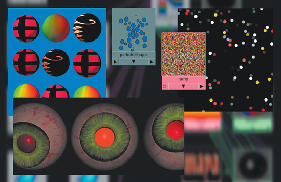
In Figure 7.3, a disco ball is given a glittery reflection. A Sampler Info utility controls the location of the glitter. The disco ball is composed of two polygon primitive spheres. The inner sphere is animated to spin. The outer sphere is static. Both spheres are faceted. (Choose Normals > Set To Face from the Polygons menu set to create the faceted effect.) The inner sphere is assigned to a Blinn material named InnerBlinn with the Color set to black and an Env Chrome texture mapped to the Reflected Color attribute. (See Chapter 5 for a discussion of environment textures.) The outer sphere is assigned to a second Blinn named OuterBlinn with a custom shading network. This network starts with the outColor of a mountain texture node connected to the colorIfTrue of a condition node. (See Chapter 8 for a description of the Condition utility.)

Figure 7.3. The glitter of a disco ball is created with the help of a Sampler Info utility. This scene is included on the CD as discoball.ma. A QuickTime movie is included as discoball.mov.
The Mountain texture has the following custom settings:
Snow Color: Black
Rock Color: White
Amplitude: 0.6
Snow Roughness: 0
Rock Roughness: 0
Snow Altitude: 1
Depth Max: 2.3
The net effect of these settings is a texture with a few white specks on a black background. The Offset V of the mountain's place2dTexture node is animated to run from 0 to 15. This rapidly changes the pattern of specks as the Timeline moves forward. The facingRatio of a samplerInfo node is connected to the firstTerm of the condition node. The outColorR of the condition node is connected to the inputR of a clamp node. The outputR of the clamp node is connected to the glowIntensity of OuterBlinn. Last, the outColor of the condition node is also connected to the incandescence of OuterBlinn.
The condition node, with the help of the samplerInfo node, tests whether or not surface normals of the outer sphere point toward the camera. If they do, they receive incandescent white specks from the mountain texture node. If they don't, they are unaffected by the condition node (the condition node's Color If False attribute is left at 0, 0, 0). Since the outputR of the clamp node is also connected to the glowIntensity of OuterBlinn, a post-process glow is placed wherever the incandescent white specks appear. The Hide Source attribute of the OuterBlinn is checked on; therefore, the glow and not the surface of OuterBlinn is rendered. The final result is a disco ball that produces small, intense bits of "reflected" light on the part that faces the camera.
Note
For an example of the Sampler Info utility used to create simulated iridescence, see section 7.1 of the Additional_Techniques.pdf file on the CD.
The Light Info utility retrieves directional and positional information from a light connected to it. The utility can function like the Light Angle option of the Ramp Shader material, but is more flexible. Before showing a few examples, however, a review of transform nodes, shape nodes, DAG objects, and instanced attributes is worth a closer look.
In Maya, cameras, lights, and surfaces are represented by two nodes: a transform node and a shape node. For example, spotlight is a transform node that carries all the light's transform information (Translate, Rotate, Scale), and spotLightShape is a shape node that possesses all the nontransform light attributes (Intensity, Cone Angle, and so on). As for geometry, nurbsSphere is the transform node, and nurbsSphereShape is the shape node.
Transform and shape nodes are also known as DAG objects. DAG (Directed Acyclic Graph) is a hierarchical system in which objects are defined relative to the transformations of their parent objects. Acyclic is a graph theory term that declares that the graph is not a closed loop. At the same time, Maya uses a dependency graph system, which simply supports a collection of nodes connected together. Technically, DAG objects are dependency graph nodes. However, not all dependency graph nodes are DAG objects since dependency graph nodes can be cyclic and do not need the parent/child relationship.
By default, there is no visible connection between a transform node and its corresponding shape node. However, every shape node must have one transform node as a parent. A transform node cannot have more than one shape node as a child, although it can have multiple transform nodes as children. A shape node is considered a "leaf level" node and cannot have any node as a child.
The worldMatrix[0] attribute, utilized by many of the example shading networks in this book, includes the [0] to indicate the index position within an array that stores the attribute. World Matrix is an "instanced attribute," whereby it can be used at different positions within a DAG hierarchy. The [n] appears automatically after a World Matrix attribute is connected in the Hypershade window. For more detailed information on the World Matrix attribute, see Chapter 8.
Directional and ambient lights do not decay naturally, nor do they possess a Decay Rate attribute. However, you can employ a Light Info, Reverse, and Set Range utility to overcome this. For example, in Figure 7.4 a directional light has an extremely short throw despite its proximity to a nearby primitive plane.
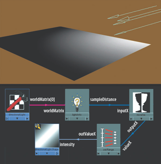
Figure 7.4. A directional light is given decay with a Light Info utility. This scene is included on the CD as directional_decay.ma.
For this to work, the worldMatrix[0] of the light's transform node is connected to the worldMatrix of a lightInfo node. The sampleDistance of the lightInfo node is connected to the inputX of a reverse node. The Sample Distance attribute returns a value that represents the distance from the connected light to the surface point being rendered. The outputX of the reverse node is connected to the valueX of a setRange node, which has its Max X attribute set to 10 and its Old Min X attribute set to −5. Last, the outValueX of the setRange node is connected to the intensity of the light's shape node. Thus, if a surface point is a great distance from the light's origin, the Intensity attribute receives a low value. If the surface point is close, it receives a high value. The following math occurs:
intensity = (((1 – sampleDistance) + 5) / 5) * 10
If the Sample Distance value is greater than 6 units, the outValueX value is negative and is thus interpreted as 0 by the light. This network functions equally well for ambient lights. For more information of the Set Range utility, see Chapter 8.
Note
You can give a Maya light a negative Intensity value, such as −1. This causes the light to negate other lights in the scene. Wherever the negative light strikes an object, it reduces the net effect of other lights in proportion to its Intensity. That said, this does not happen if the light is connected to a shading network similar to the one described in this section. Instead, the negative Intensity value is essentially clamped to 0.
In Figure 7.5, a NURBS squid begins to glow once a light has passed it by. This trait, known as phosphorescence, is normally caused by the emission of light following the removal of a radiation source. In this reproduction, a standard spot light serves as the "radiation." The spot light's Intensity attribute is set to 15 and its Decay Rate is switched to Linear, forcing the light to have a fairly short throw.
The squid is assigned to a shading network that starts with a Light Info utility. The worldMatrix[0] of the spotLightShape node is connected to the worldMatrix of a lightInfo node. The sampleDistance of the lightInfo node is connected to the input1X of a multiplyDivide node. The outputX of the multiplyDivide node is connected to the glowIntensity of a blinn material node. The Input2X of the multiplyDivide node is set to 1000, and the Operation attribute is set to Divide. Dividing by a large number allows the glow of the blinn node to increase as the light moves farther away but will never allow the glow value to become excessively large.

Figure 7.5. A Light Info utility allows a squid to glow when a spot light is withdrawn from its presence. A simplified version of this scene is included on the CD as glow.ma. A QuickTime movie is included as glow.mov.
The sampleDistance of the lightInfo node is also connected to the valueY of a setRange node (see Chapter 8 for a description of the Set Range utility). The outValue of the setRange node is connected to the ambientColor of the blinn node. This increases the amount of greenish ambience as the light gets farther away. The setRange Old Max attribute is set to 100, 100, 100 and the Max attribute is set to 0, 2, 0. Hence, if the light is 0 units from the squid, the Ambient Color is 0, 0, 0. If the light is only 50 units from the squid, the Ambient Color is 0, 1, 0. If the light is 100 units from the squid, the Ambient Color is 0, 2, 0.
In a second example of the Light Info utility, a camera is connected in order to retrieve world space directional information. This information is then used to control the color of an "in camera" display. In Figure 7.6, the worldMatrix[0] of the default camera's perspShape node is connected to the worldMatrix of a lightInfo node. The camera's worldMatrix[0] is also connected to the matrix of a vectorProduct node. The lightDirection of the lightInfo node is connected to the input1 of the vectorProduct node as well.

Figure 7.6. An "in camera" display that indicates which direction a camera is pointing is created with a Light Info utility. This scene is included on the CD as camera_display.ma. A QuickTime movie is included as camera_display.mov.
The Vector Product utility is designed to perform mathematical operations on two vectors. In addition, it can multiply a vector by a matrix. This function allows the Vector Product utility to convert a vector in one coordinate space to a second coordinate space. In this case, the vectorProduct node's Operation attribute is set to Vector Matrix Product, which undertakes this task. Since the worldMatrix[0] of the camera is used as the input matrix, the output of the vectorProduct node is the camera direction vector in world space. The output vector runs between −1, −1, −1 and 1, 1, 1 in X, Y, and Z. (For a deeper discussion on vectors and vector math, see Chapter 7.)
Note
If lightDirection is connected directly to either multiplyDivide node, the network will not function. Instead, the minus sign will remain blue regardless of camera rotation. This indicates that the lightInfo node outputs a 0, 0, 1 vector, which infers that the camera lens is pointing down the negative Z axis with no rotation in X or Y (which is the same as the default state of a new camera).
The output of the vectorProduct node is connected to the input1 attributes of two multiplyDivide nodes. The multiplyDividePlus node has its Input2 set to −1, −1, −1, guaranteeing that it produces a negative value. The multiplyDivideMinus node has its Input2 left at 1, 1, 1. Last, the output of each multiplyDivide node is connected to the outColor of two different surface shader material nodes. The PlusColor material is assigned to a plus sign created as a text primitive. The MinusColor material is assigned to a minus sign. Both signs are placed near the bottom of the camera and parented to the camera itself. As the camera is rotated, the colors of the symbols change in correspondence to the direction the camera points. (If the colors are not visible with Hardware Texturing checked on, you will have to render out a test frame.)
As with the axis display found in Maya's workspace views, red corresponds to X, green corresponds to Y, and blue corresponds to Z. Hence, if the camera points in the positive X direction, the plus sign becomes red. If the camera points in the negative X direction, the minus sign becomes red. Table 7.1 reveals what happens mathematically when the camera is given other rotations.
Table 7.1. Colors resulting from different camera rotations.
Camera rotation | vectorProduct output | MinusColor RGB (output × 1, 1, 1) | PlusColor RGB (output × −1, −1, −1) |
|---|---|---|---|
0, 0, 0 | 0, 0, 1 | 0, 0, 1 (bright blue) | 0, 0, 0 (black) |
45, −45, 0 | −0.5, −0.7, 0.5 | 0, 0, 0.5 (blue) | 0.5, 0.7, 0 (yellow-green) |
−90, 0, 0 | 0, 1, 0 | 0, 1, 0 (bright green) | 0, 0, 0 (black) |
Any RGB value less than 0 is clamped to 0 by the renderer (negative color values are rendered black). You can use this coloring technique on any object (as can be seen by the two primitive shapes in the camera's view). In addition, you can connect any object that possesses a World Matrix attribute—such as a camera, light, or NURBS surface—to the Light Info and Vector Product utilities so that its direction can be derived in this fashion.
The Particle Sampler utility has the unique ability to graft a UV texture space onto a particle mass. Before I suggest specific applications, however, let's take a quick look at particle texturing.
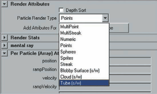
In Maya, particles are either hardware or software rendered. This section focuses on software-rendered particles since they can accept standard materials. The three software-rendered particle types are Blobby Surface, Cloud, and Tube. Their software-rendering capability is symbolized by the "s/w" beside the particle name listed by the Particle Render Type drop-down menu, which is found in the Render Attributes section of the particle shape node Attribute Editor tab (see Figure 7.7). Although Cloud particles are excellent for smoke, Blobby Surface particles can replicate a wide range of liquid and semiliquid materials.
By default, Blobby Surface particles derive their color from the lambert1 material via the initialParticleSE (Initial Particle Shading Engine) shading group node. You can assign Blobby Surface particles to Lambert, Blinn, Phong, Phong E, Anisotropic, Layered Shader, and Ramp Shader materials.
Cloud and Tube particles derive shading information from the default particleCloud1 material (see the next section). Cloud and Tube particles cannot be assigned to any other standard material. However, you can assign the particles to a new Particle Cloud or Volume Fog material (found in the Volumetric section of the Create Maya Nodes menu).
To apply a texture to a Cloud or Tube particle, you can map the Color or Life Color attribute of a Particle Cloud material. If you map the Color, the texture is applied to each particle but will be oriented toward the camera. For example, in Figure 7.8 a Checker texture with a Repeat UV of 1, 1 is used.
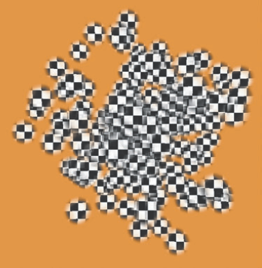
Figure 7.8. A Checker texture material is mapped to the Color attribute of a Particle Cloud material. This scene is included on the CD as cloud_checker.ma.
On the other hand, if you map a texture to the Life Color attribute, colors are sampled along the V axis of the texture. To create an example, follow these steps:
Switch to the Dynamics menu set. Choose Particles > Create Emitter. Play back the Timeline until the particles are visible.
Select the particles. Press Ctrl+A to open the Attribute Editor. Switch to the particleShape1 tab. Scroll down to the Render Attributes section and change Particle Render Type to Cloud (s/w). Click the Current Render Type button and reduce the Radius value so that individual particles are easier to see.
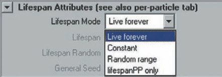
Go to the Lifespan Attributes section and change Lifespan Mode to Constant (see Figure 7.9). Change Lifespan to 5 so that the particles live 5 seconds. If Lifespan Mode is set to the default Live Forever option, Life Color cannot use the ramp color information.
Open the Hypershade window. Choose the particleCloud1 material and bring up its Attribute Editor tab. Click the checkered Map button beside Life Color and choose a Ramp texture from the Create Render Node window.
A ramp node is connected to the particleCloud1 material. However, it is represented by a spherical icon. In addition, a Particle Sampler utility is connected to the ramp. Render a test. Young particles render red (see Figure 7.10). Old particles render blue. An example scene is included as
cloud_ramp.main the Chapter 7 folder on the CD.

In contrast, a Blobby Surface particle node that is assigned to a material that uses a texture will pick up that texture. Oddly enough, each particle receives the entire texture twice—once for the top and once for the bottom (see Figure 7.11). In addition, the Blobby Surface particles will show bump and transparency maps. The texture will appear even when the Threshold attribute is raised and the particles begin to stick together.
You can prevent each Blobby Surface particle from carrying the complete texture by manually assigning the node to a shading network that uses a Particle Sampler utility. For example, in Figure 7.12 a NURBS plane is used as an Emit From Object particle emitter. The Emitter Type attribute of the emitter is set to Directional. Rate (Particles/Sec) is set to 25. Direction X, Direction Y, and Direction Z are set to 0, 1, 0, respectively. Speed is set to 1. The particleShape's Particle Render Type attribute is set to Blobby Surface with a Radius value of 0.1 and a Threshold value of 0.5. The particleShape's Lifespan Mode attribute is set to Constant with a Lifespan value of 1.
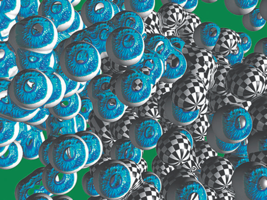
Figure 7.11. One Blobby Surface particle node is assigned to a Phong material with a Checker texture. A second is assigned to a Phong with an iris bitmap. This scene is included on the CD as particle_eye.ma.

Figure 7.12. A Blobby Surface particle mass picks up the red and blue of a Checker texture with the help of a Particle Sampler utility. This scene is included on the CD as particle_checker.ma.
As for the shading network, a red and blue Checker texture is mapped to the Color of a Phong material. The Phong is assigned to the Blobby Surface particle node. The outUvCoord of a particleSamplerInfo node is connected to the uvCoord of the checker's place2dTexture node. (The UV Coord attribute is hidden until you choose Right Display > Show Hidden in the Connection Editor.) This connection fits the UV texture space of the checker node to the particle mass. As with the Life Color attribute of the Particle Cloud material, the texture is sampled at a single point along the V direction during the particle's life. Hence, details in the U direction (left to right on the screen) are lost. The relatively high particle count and a Threshold value of 0.5 turns the blue of the checker texture into thin horizontal lines.
You can correct the U direction smearing with a slight change to the connections. In Figure 7.13, a similar shading network is laid out. This time, instead of a Checker texture, a bitmap of the word Maya is loaded into a File texture. The outVCoord of a particleSamplerInfo node is connected directly to the vCoord of the file texture node. The outUCoord attribute, however, is not connected at all. Instead, the worldPositionZ of the particleSamplerInfo node is connected to the input1X of a multplyDivide node. The outputX of multiplyDivide is connected to the uCoord of the file node. Since the particles are born along the Z axis of the world, the worldPositionZ attribute serves as a crude Repeat U tiling control. The Input2X attribute of the multiplyDivide node is set to 0.08, which creates the following math:
uCoord = worldPositionZ x 0.08

Figure 7.13. Blobby Surface particles display the word Maya with the help of a Particle Sampler utility. This scene is included on the CD as particle_word.ma. A QuickTime movie is included as particle_word.mov.
If a particle is born at the far right of the emitter, it has a Z position of 12. Hence, the uCoord becomes roughly 1, which is the right edge of the Maya bitmap. If the Z position is 6, the uCoord becomes roughly 0.5, or the center of the bitmap. This technique works with particles that have a chaotic or random motion (although the texture will be more difficult to recognize and will ultimately repeat). In addition, this technique works when the Blobby Surface particle Threshold value is raised and the particles begin to stick together.
The Particle Sampler utility can also command various per-particle attributes. For a discussion of this feature and the Array Mapper utility, see Chapter 8.
The Distance Between utility does exactly what its name implies. It returns a value that represents the distance between any two objects. You can automatically apply this utility by choosing Create > Measure Tools > Distance Tool and clicking in two different locations in any workspace view. Two locators are placed in the scene, and the distance is measured between them by a Distance Between utility. The distance value is displayed on a line drawn between the two locators. Although this method is convenient, it is possible to manually connect a Distance Between utility to a custom shading network.
For example, in Figure 7.14 the color of two primitive polygon shapes changes from blue to red as they approach each other. In this shading network, the center attribute of ShapeA's transform node is connected to point2 of a distanceBetween node. The center of ShapeB's transform node is connected to point1 of the distanceBetween node (the Translate attribute will not work in this case). The distance attribute of the distanceBetween node is connected to the input1X of a multiplyDivide node. The Input2X attribute of the multiplyDivide node is set to 0.05, guaranteeing that the result will be well below 1 even when the shapes travel a significant distance apart. The outputX of the multiplyDivide node is connected to the inputX of a reverse node. This ensures that the shapes will become redder as they approach each other and not vice versa. Last, the output of the reverse node is connected to the color of a blinn material node. The InputY and InputZ attributes of the reverse node are set to 0.5 since they have no inputs. This creates the green-blue color when the ouputX of the multiplyDivide node, which controls the inputX of the reverse node, provides a low value.
Custom connections are not limited to materials, textures, and geometry transform nodes. Any node that can be MMB-dragged from the Hypergraph to the Hypershade is fair game. A few examples that employ geometry, cameras, construction history, and default shading nodes follow.
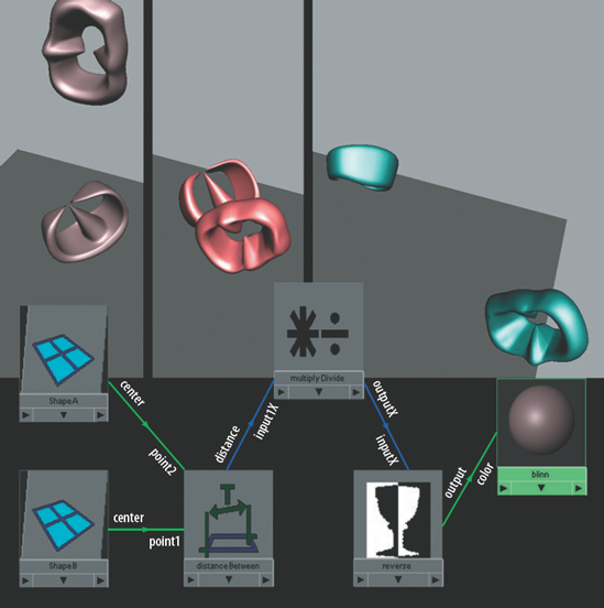
Figure 7.14. The colors of two abstract shapes are controlled by a Distance Between utility. This scene is included on the CD as distance.ma. A QuickTime movie is included as distance.mov.
A spinning plane propeller is basically a blurred disc. Although the prop is visible with the correct point-of-view or proper frame rate, its shape is generally indistinct. You can emulate a spinning propeller in Maya by having a propeller disc drive its own transparency. For example, in Figure 7.15 a NURBS disc is animated rotating from 0 to 10,000 degrees in Z over a period of 90 frames.

Figure 7.15. A NURBS disc serves as a spinning propeller. The opacity flicker is driven by its own geometry. The yellow arrow indicates the point at which Maya inserts a unitConversion node. A simplified version of this scene is included on the CD as propeller.ma. A QuickTime movie is included as propeller.mov.
The rotateZ of the disc's transform node is connected to the input1X of a multiplyDivide node named multiplyDivide1. The outputX of multiplyDivide1 is connected to the input1X of a second multiplyDivide node named multiplyDivide2. The Input2X of multiplyDivide1 is set to 0.01. The Input2X of multiplyDivide2 is set to 0.005. This sequence converts a potentially large rotation value into an extremely small one. The outputX of multiplyDivide2 is connected to the offsetU of the place2dTexture node belonging to a fractal texture node. Thus, the rotation of the disc automatically pushes the fractal texture node in the U direction. The Repeat UV of the place2dTexture node is set to 0.001, 0.001, which reveals only a small section of the fractal. The custom settings for the fractal texture node are as follows:
Ratio: 0.5
Frequency Ratio: 10
Bias: −0.3
Filter: 5
These adjustments create a softer version of the fractal pattern. The outColor of the fractal node is connected to the transparency of a blinn material node named PropellerColor. As the disc rotates, the fractal moves left, revealing darker and lighter sections. Hence, the propeller disc flickers during the animation. The color of the disc is derived from a circular ramp texture with brown and yellow handles. The ramp is projected onto the disc for a more exact lineup of colors. While this technique might not work for close-ups, it can be used successfully for wider shots and flybys. It also serves as an extremely efficient method of rendering since no motion blur is involved.
Alfred Hitchcock introduced a famous zoom-dolly camera move in the film Vertigo (1958). Steven Spielberg later popularized the same motion in Jaws (1978). If a camera zooms out while simultaneously dollying forward, the background distorts over time. This is due to the optical nature of the camera lens. Telephoto lenses (for example, 300 mm) flatten a scene, but wide lenses (for example, 24 mm) give a scene more depth. It's possible to change the focal length of a zoom lens with a twist of the hand (for example, 200 mm to 50 mm).
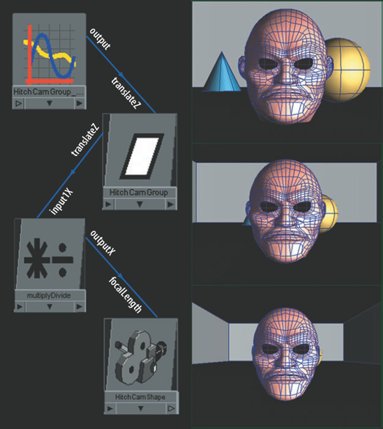
You can automate the Hitchcock zoom-dolly with custom connections. For example, in Figure 7.16 the transform node of a single-node camera, named HitchCam, is parented to a group node named HitchCamGroup. To view the custom shading network, open hitchcock.ma and follow these steps:
Open the Hypershade window and switch to the Utilities tab.
MMB-drag the multiplyDivide node into the work area.
With the multiplyDivide node selected, click the Input And Output Connections button.
HitchCamGroup is animated along the Z axis. HitchCamGroup's translateZ attribute is connected to the input1X of the multiplyDivide node. The outputX of the multiplyDivide node is connected to the focalLength of the camera's shape node, named HitchCamShape. The multiplyDivide node's Operation is set to Multiply, and its Input2X is set to 10. When HitchCamGroup is at its start position of 0, 1, 10, the focalLength of HitchCamShape is 100. When HitchCamGroup is at its end position of 0, 1, 1, the focalLength of HitchCamShape is 10. Scrubbing the Timeline will quickly show the high degree of distortion that happens to the background and foreground objects. An animation curve node—seen at the top of the network—appears because an attribute is keyframed. Even though HitchCamGroup is the parent of HitchCam, there is no visible connection in the Hypershade window.
Note
Strangely enough, it is possible to connect a node to itself. MMB-dragging a node on top of itself is the quickest way to do this. Choosing Other from the Connect Input Of menu opens the Connection Editor and reveals that the node is listed in both the Output and the Input column. That said, an attribute cannot be connected to itself (for example, focalLength to focalLength). Nevertheless, two different attributes can be connected (for example, focalLength to shutterAngle).
You can put construction history nodes to work in the Hypershade window. In Figure 7.17, an asteroid model automatically receives more surface detail as it approaches the camera along the X axis.
To view the entire custom network, open history.ma and follow these steps:
Open the Hypershade window and switch to the Utilities tab.
MMB-drag the clamp node into the work area.
With the clamp node selected, click the Input And Output Connections button. A portion of the network becomes visible.
Select all the visible nodes and click the Input And Output Connections button a second time.

Figure 7.17. A polygon asteroid receives more detail as it approaches the camera. Iterations of a Smooth tool are driven by custom connections. This scene is included on the CD as history.ma. A QuickTime movie is included as history.mov.
For the network to function, the animated translateX attribute of the pSphere polygon transform node is connected to the input1X of a multiplyDivide node. The multiplyDivide node's Operation is set to Divide and its Input2X attribute is set to 15. This division increases the amount of distance the asteroid must travel before the detail is increased. The outputX of the multiplyDivide node is connected to the inputR of a clamp node. The outputR of the clamp node is connected to the divisions attribute of a polySmoothFace node. The polySmoothFace node is a product of choosing Mesh > Smooth. Whenever the Smooth tool is applied, it creates two new nodes: polySmoothFace and polySurfaceShape. The Divisions attribute of polySmoothFace controls the number of iterations the Smooth tool undertakes. The clamp node's MaxR attribute is set to 3 so that the iterations stay between 0 and 3. The surface's pre-Smooth state is retained by polySurfaceShape. Both polySmoothFace and polySurfaceShape nodes, like all construction history nodes, will exist until history has been deleted on the polygon surface (Edit > Delete By Type > History).
By default, Maya assigns all new geometry to the Initial Shading Group and the Lambert material connected to it (named lambert1). You can replace the Lambert with a Blinn or any other material by deleting the connection between the outColor of the default lambert material node and the surfaceShader attribute of the initialShadingGroup node. You can locate the initialShadingGroup node by clicking the Input And Output Connections button while lambert1 is selected. You can then connect the outColor of a new material to surfaceShader of the initialShadingGroup. From that point forward, all new surfaces are automatically assigned to the new material (see Figure 7.18). The outColor of the default lambert material node is also connected to the surfaceShader of the initialParticleSE node. A different material can be connected to this as well. The initialParticleSE node determines the default material qualities of software-rendered Blobby Surface, Cloud, and Tube particles.
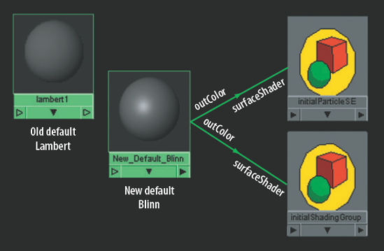
Figure 7.18. The default Lambert material is replaced with a Blinn. This scene is included on the CD as initial_shading.ma.
Note
Whenever a new material is assigned to a surface, it automatically receives its own shading group node with a name along the lines of blinn1SG. These material-specific shading group nodes can be deleted and replaced if necessary. For additional information on shading groups, see Chapter 4.
A custom shading network is not limited to a single material. In some situations, connecting one material to a second material can force the renderer to apply an additional layer of evaluation to the assigned surface. As a simple demonstration of this, the outColor of a phong material node is connected to the color of a lambert material node (see Figure 7.19). Although the lambert node does not have the ability to produce a specular highlight, it picks up the look of a specular highlight from the phong.

To achieve this, the renderer evaluates the assigned surface as if a Phong material was assigned to it. The renderer takes the color information from this evaluation and applies it to the color of the Lambert material. This evaluation occurs at each pixel and the color is assigned at each pixel. If a pixel is white with the Phong shading model, then the Lambert color is white. Hence, a false specular highlight is produced. Any attribute of the phong material node that is mapped will carry through. For example, if a texture is mapped to the Bump Mapping attribute of the phong node, the bump will appear automatically on the lambert node.
Note
For a demonstration of a complex, custom skin shader that uses the majority of techniques in this chapter (including multiple materials), see section 7.2 of the Additional_Techniques.pdf file on the CD.
Studio Clear Coat is a plug-in utility that's in its own category. Its sole function is to create reflections with uneven intensity. As opposed to the car paint shading network detailed in Figure 7.2, this utility functions as a single node.
For example, in Figure 7.20 the outValue of a studioClearCoat node is connected to the reflectivity of a blinn material node (named Car_Paint). The same lighting and environment that was used in Figure 7.2 is applied here. The studioClearCoat node has an Index value of 1.7, a Scale value of 1.55, and a Bias value of −0.1. The resulting render is almost identical to Figure 7.2. The main difference is the rapidity with which the Studio Clear Coat utility transitions between the hood reflection and fender reflection. Although this is not necessarily better or worse, the Studio Clear Coat utility is extremely easy to apply. Unfortunately, it will not work with the mental ray renderer. The custom paint network used in Figure 7.2, on the other hand, offers more flexibility with the addition of the Value gradient and will work with Maya software or mental ray renderers.

Figure 7.20. The reflective falloff of car paint is controlled by a Studio Clear Coat utility. A simplified version of the scene is included on the CD as clearcoat.ma.
The Studio Clear Coat utility's attributes follow:
- Index
Represents the refractive index of the surface. A refractive index is a constant that relates the speed of light through a vacuum to the speed of light though a material (such as car paint). The constant follows:
speed of light through a vacuum
÷
speed of light through a material
Water has a refractive index of 1.33, which equates to
1/0.75. The speed of light through water is only 0.75 times as fast as the speed of light through a vacuum. The refractive index of air is extremely close to 1 and is considered 1 when working in 3D.As light passes between two materials that possess different refractive indices, the angle of refraction does not match the angle of incidence (the angle between the incoming light ray and the material boundary normal, which is perpendicular to the boundary surface). If the light passes from a material with a low refractive index to a high refractive index, the angle of refraction is rotated toward the material boundary normal. Hence, objects appear bent (for example, when a pole is dipped into water). The clear-coat paint systems on modern cars produce a refractive index somewhere between 1.4 and 1.8. The amount of perceived distortion is minimized by the extreme thinness of the transparent clear-coat layer (an average of 50 to 100 microns).
- Scale
Serves as a multiplier for the final result. Higher values will make the reflection more intense.
- Bias
Offsets the intensity of the reflection. Lower values decrease the intensity of the reflection and increase the contrast within the reflection. Higher values increase the intensity and lower the contrast. The default value is −0.1.
Note
If the Studio Clear Coat utility is not visible in the General Utilities section of the Hypershade window, choose Window > Settings/Preferences > Plug-In Manager and click the Loaded check box for the clearcoat.mll plug-in.
Note
Refractive indices are derived from Snell's Law, which describes the relationship between angles of incidence and angles of refraction. The law is named after Willebrord Snell (1580–1626), who developed a mathematical model based on earlier investigations by Claudius Ptolemy (ca. 100–170) and others. For more information on Snell's Law, see Chapter 12.
In this tutorial, you will create a custom cartoon shading network that combines solid colors with a simulated halftone print (see Figure 7.21). Sampler Info, Surface Luminance, Condition, and Multiply Divide utilities will be used.

Figure 7.21. A custom cartoon shading network applied to primitives. A QuickTime movie is included on the CD as cartoon.mov.
Create a new Maya scene. Open the Hypershade window.
MMB-drag a Surface Shader material into the work area and rename it Cartoon. MMB-drag a Condition utility (found in the General Utilities section of the Create Maya Nodes menu) into the work area. Place it to the left of the Cartoon node. Use Figure 7.22 as a reference.
Connect the outColor of the condition node to the outColor of the Cartoon node. You will have to open the Connection Editor to do this.
Select the condition node and rename it ConditionA. Open its Attribute Editor tab. Click the Color If False Map button and choose a Ramp texture from the Create Render Node window. A place2dTexture node will automatically appear with the new ramp node. Rename the ramp node RampA.
Select RampA and open its Attribute Editor tab. Create four color handles that go from black to green to white (see Figure 7.23). Change RampA's Interpolation attribute to None.
MMB-drag a Surface Luminance utility (found in the Color Utilities section of the Create Maya Nodes menu) into the work area. Place it to the left of the other nodes. Connect the outValue of the surfaceLuminance node to the firstTerm of ConditionA.
Connect the outValue of the surfaceLuminance node to the vCoord of RampA. You will have to use the Connection Editor. This connection forces the render to select different pixels in the V direction of the ramp based on the amount of light any given point on the assigned surface receives. If a surface point is dark, it gets its color from the bottom of the ramp. If a surface point receives a moderate amount of light, it gets its color from the center of the ramp.
MMB-drag a second Condition utility into the work area. Place it to the left of ConditionA. Rename the new condition node ConditonB. Connect the outColor of ConditionB to colorIfTrue of ConditionA.
MMB-drag a Sampler Info utility (found in the General Utilities section of the Create Maya Nodes menu) into the work area. Place it to the left of ConditionB. Connect the facingRatio of the samplerInfo node to the firstTerm of ConditionB.
Select ConditionB and open its Attribute Editor tab. Set the Color If False attribute to 0, 0, 0. Click the Color If True Map button, select As Projection in the 2D Textures section of the Create Render Node window, and click the Ramp texture button. Selecting As Projection creates the Ramp texture with a projection node and a place3dTexture node (see Figure 7.22). Rename the new ramp node RampB.
Create a new one-node camera by choosing Create > Cameras > Camera from the main Maya menu. Create several primitives and place them in the view of the camera. Assign all the primitives to the Cartoon material. Feel free to change the camera's Background Color attribute to white or add a white ground plane.
Select the projection node and open its Attribute Editor tab. Change the Proj Type attribute to Perspective. MMB-drag the new camera node, named camera, from the Cameras tab area to the work area and drop it on top of the projection node. Choose Other from the Connect Input Of drop-down menu. The Connection Editor window opens. Connect the Message of the camera node to the linkedCamera of the projection node. The Message attribute is normally hidden. When you choose Left Display > Show Hidden in the Connection Editor, the Message attribute becomes visible at the top of the list. When the camera node is connected to the projection node, the projection node will know to project from the view of the new camera and not the default persp camera.
Look at the camera icon in a workspace view. There should be a projection frustum (a pyramid shaped icon representing a camera's view) extending from the camera icon toward the primitive objects (Figure 7.24). If not, select the place3dTexture node that is connected to the projection node. This will select the frustum icon and allow you to translate it to a suitable location. If you would like to animate the camera moving, parent the place3dTexture node to the camera. Ultimately, this projection will allow the halftone dots to appear continuously across multiple surfaces without distortion.
Select RampB and open its Attribute Editor tab. Place two color handles in the color field. A black handle should be at the bottom. A dark purple handle should be at the center (Figure 7.23). Set Type to Circular Ramp and Interpolation to None. RampB will produce a halftone print pattern. Select the place2dTexture node of RampB. Open its Attribute Editor tab and change the Repeat UV value to 65, 40. Choose larger numbers to create smaller halftone circles.
Select ConditionB and open its Attribute Editor tab. Set the Second Term attribute to 0.3 and the Operation to Greater Than. ConditionB works as an if statement. If the facingRatio of the samplerInfo node is greater than 0.3, ConditionB will output the halftone pattern of RampB as the color. If the facingRatio is 0.3 or less, pure black will be output as the color; ultimately, this creates a black "ink line" around the edge of the objects.
Select ConditionA and open its Attribute Editor tab. Set the Second Term attribute to 0.5 and the Operation to Less Than. ConditionA serves as a second if statement. If the outValue of the surfaceLuminance node is less than 0.5, the color output by ConditionB is selected (black or halftone dots). If the outValue of the surfaceLuminance node is equal to or greater than 0.5, the color output by RampA (various shades of green) is selected. The surfaceLuminance node also controls the vCoord of RampA, so that the selection of different shades of green is based on the amount of light the surface receives.
The custom cartoon material is complete! Render out a test. It should look similar to Figure 7.21. If you get stuck, a finished version of the material is saved as
cartoon.main the Chapter 7 scene folder on the CD.