Math utilities refine outputs and emulate complex mathematics. Switch utilities let you create numerous texture variations with a single material. With Array Mapper and Particle Sampler utilities, you can control a particle's material and movement on a per-particle basis. You can also create unique effects with Stencil and Optical FX utilities.
Chapter Contents
Practical applications of each math utility
A general approach to using per-particles attributes
The functionality of the Array Mapper and Particle Sampler utilities
Uses for Stencil and Optical FX utilities
The purpose of Unit Conversion and other scene nodes
The values provided by various attributes in Maya are often unusable in a custom shading network. The numbers are too large, too small, or negative when they need to be positive. Hence, Maya provides a host of math utilities designed to massage values into a usable form. The utilities vary from simple (Reverse, Multiply Divide, and Plus Minus Average) to advanced (Array Mapper, Vector Product, and others). Switch utilities, on the other hand, provide the means to texture large groups of objects with a limited number of materials.
The Reverse utility simply reverses an input. The following math occurs:
Output= 1 -Input
Thus, an input of 1 produces 0 and an input of 0 produces 1. At the same time, the Reverse utility will make larger numbers negative or positive. For instance, an input of 100 produces −99 and an input of −100 produces 101. Only an input of 0.5 will lead to an unchanged output.
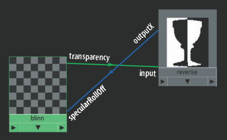
For example, in Figure 8.1 the Specular Roll Off of a material is automatically reduced as it becomes more transparent. The transparency attribute of a blinn material node is connected to the input of a reverse node. The outputX of the reverse node is connected back to the specularRollOff of the blinn. If a vector attribute (RGB) is connected to the reverse node, it is not necessary to utilize all three channels on the output. Without this network, a specular highlight of the blinn will remain visible even if its transparency is turned up to 100 percent. Although you can keyframe the Specular Roll Off attribute, this network is easy to set up.
The Multiply Divide utility applies multiplication, division, or power operations to zero, one, or two inputs. If no inputs exist, you can enter numbers into the Input1 and Input2 attribute fields. If the Multiply Divide utility has one input, you can enter numbers into the unconnected Input1 or Input2 attribute fields. Regardless of the number of inputs, the Multiply Divide utility follows this logic:
Input1/Input2Input1*Input2Input1^Input2
If the utility's Operation attribute is set to Multiply, the order makes no difference. If the utility's Operation is set to Divide or Power, however, the order is critical, as in this example:
10 / 2 = 5 while 2 / 10 = 0.2
10 ^ 2 = 100 while 2 ^ 10 = 1024
A chain of Multiply Divide nodes can emulate fairly complex math. Although Maya expressions can easily handle math work, the Multiply Divide utility offers an alternative method that allows the user to stay within the Hypershade window. For example, in Figure 8.2 the generic formula y = 1 / (x^(x / 2)) is re-created.
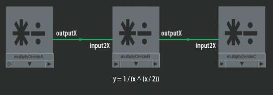
Figure 8.2. A generic formula is re-created with Multiply Divide utilities. This network is included on the CD as multiply_generic.ma.
To view the custom network, follow these steps:
In this case, (x / 2) is provided by multiplyDivideA. x is entered manually into the Input1X field. Input2X is set to 2. The Operation attribute is set to Divide.
x ^ is provided by multiplyDivideB. x is entered manually into the Input1X field. The Operation attribute is set to Power. outputX of multiplyDivideA is connected to input2X of multiplyDivideB.
1 / is provided by multiplyDivideC. Input1X is set to 1. Operation is set to Divide. outputX of multiplyDivideB is connected to input2X of multiplyDivideC. Ultimately, outputX of multiplyDivideC equals the answer, or in this case, y. If x is 1, then y equals 1. If x is 4, then y equals 0.0625. If x is 15, then y = 1.51118e-009. In Maya, e-009 is equivalent to ×10−9. If the outputX of multiplyDivideC is connected to the input1X of a fourth multiplyDivide node, the input1X field will display 0.000. Since the Input1 and Input2 fields of the Multiply Divide utility are limited to three floating points, they will not display numbers with an excessive number of digits. However, the correct value of multiplyDivideC's outputX can always be retrieved by entering getAttr multiplyDivideC.outputX in the Script Editor.
Note
For an additional application of the Multiply Divide utility, see section 8.1 of the Additional_Techniques.pdf file on the CD. In section 8.1, the rotation of a tire is automatically and accurately driven by its translation.
The Plus Minus Average utility supports addition, subtraction, and average operations. It operates on single, double, and vector input attributes. If single attributes are connected, they are not visible in the Plus Minus Average utility's Attribute Editor tab. However, double and vector attributes are indicated by input fields (see Figure 8.3).
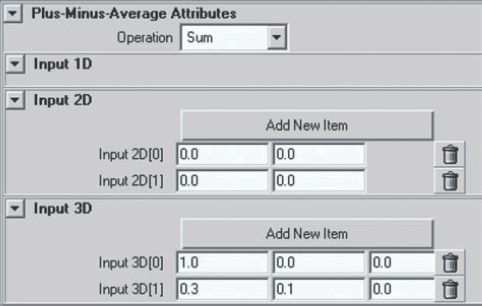
The Plus Minus Average utility provides Add New Item buttons in the Input 2D and Input 3D sections of its Attribute Editor tab. When you click one of these buttons, a new set of input fields is added to the appropriate section. The input fields are not connected to a node, which allows you to enter values by hand. However, you can choose to make a custom connection to the new input.
You can connect single attributes to input1D[n] of a plusMinusAverage node. You can connect double attributes, such as uvCoord, to input2D[n]. You can connect vector attributes, such as outColor, to input3D[n]. n represents the order with which attributes have been connected, with the [0] position being the first. There is no limit to the number of attributes that may be connected. For example, in Figure 8.4 the translateX attributes of four primitive polygon shape transform nodes are connected to input1D[n] of a plusMinusAverage node with the node's Operation set to Subtract. To illustrate the result, the output1D of the plusMinusAverage node is connected to the translateX of a locator. To see this custom network, follow these steps:
Open the
plus_simple.mafile from the CD. Open the Hypershade window and switch to the Utilities tab.MMB-drag plusMinusAverage1 into the work area.
With plusMinusAverage1 selected, click the Input And Output Connections button. The network becomes visible.

Figure 8.4. Two Plus Minus Average utilities subtract translation and average texture color for four polygon shapes. This scene is included on the CD as plus_simple.ma.
The locator position represents the result of the following math:
shape1.tx - shape2.tx - shape3.tx - shape4.tx
If the Operation attribute of the plusMinusAverage node is switched to Sum, the same logic applies. However, if the Operation attribute is switched to Average, the following math occurs:
(shape1.tx + shape2.tx + shape3.tx + shape4.tx) / 4
You can apply the Average operation to color attributes as well. In the same example, the outColor attributes of four textures are connected to the input3D[n] of a second plusMinusAverage node. The utility's output3D is connected to the color of a blinn material node, which is assigned to all four shapes. The following happens to the red channel of an individual pixel:
(water.colorR + ramp.colorR + mountain.colorR + bulge.colorR ) / 4
Note
For an additional application of the Plus Minus Average utility, see section 8.2 of the Additional_Techniques.pdf file on the CD. In section 8.2, the length of a triangle's edge is solved with the application of the Pythagorean Theorem.
Maya expressions offer the most efficient and powerful way to incorporate math calculations into a custom shading network. Although a deeper discussion on expressions is beyond the scope of this book, here are a few items to keep in mind:
- Create New Expression
Right-clicking an attribute field in the Attribute Editor and choosing Create New Expression from the shortcut menu opens the Expression Editor window. The attribute that was chosen will be highlighted in Expression Editor's Attributes list. Once a valid expression is created and the Create button is clicked, an expression node and appropriate connections are created. The attribute field, as seen in the Attribute Editor, turns purple to indicate the connection to an expression. The expression node is not immediately visible in the Hypershade work area. However, if you select the node to which the expression was applied in the work area and click the Input And Output Connections button, the expression node is revealed.
- Time
A master Time node (time1) is automatically connected to each expression node and is undeletable. This node manages the flow of time for the Maya Timeline. You can connect the node's outTime to any single attribute of any node; however, a connection line will not necessarily appear in the Hypershade window.
- Nodes and Channels
You can reference any channel of any node in an expression. The naming convention will always follow the formula node.channel.
- Functions
For a list of Maya math, vector, array, and other functions available to expressions, choose the Insert Functions menu of the Expression Editor window.
- Duplication
You can duplicate expression nodes by choosing Edit > Duplicate > Without Network from the Hypershade window menu. The new expression appears in the Expression Editor if you choose Select Filter > By Expression Name from the Expression Editor menu. The math functions of the duplicate are identical to the original. However, the channel names are missing. You can display the new expression node by entering the node name, such as expression3, into the search field of the Hypergraph Connections window.
The Set Range utility maps one range of values to a second range of values. The underlying math for the utility follows:
outValue=Min+ (((value-oldMin)/(oldMax-oldMin)) * (Max-Min))
As an example illustrated by Table 8.1, five different ValueX inputs are processed by a Set Range utility, resulting in new Out ValueX outputs. For this example, Old MinX of the utility is set to −100, Old MaxX is set to 100, Min X is set to 0, and MaxX is set to 1.
Table 8.1. The Result Of Various ValueX Inputs Applied To A Set Range Utility
ValueX | −100 | −75 | 0 | 21 | 500 |
Out ValueX | 0 | 0.125 | 0.5 | 0.605 | 1 |
The mid-value of the Old MinX and Old MaxX range (0) becomes the mid-value of the new MinX and MaxX range (0.5). Any value greater than the Old MaxX is clamped to the Old MaxX value before it is remapped. Hence, 500 becomes 100, which is then remapped to 1. Min, Max, Old Min, Old Max, and Value are vector attributes. The individual channels (for example MinX, MinY, MinZ) can carry different values.
In a working example, the Set Range utility is used to create diffuse shadows on a directional light. Diffuse shadows are a product of diffuse lighting. A diffuse light source is one that either produces divergent light rays or is physically large enough that it produces multiple overlapping shadows. One feature of a diffuse shadow is an increased edge softness over distance. A second feature is a shadow color that becomes lighter over distance (see the photo at the top of Figure 8.5).
Since depth map shadows are calculated using a single point-of-view of a light, Maya is unable to produce a diffuse effect. A light's Filter Size attribute blurs the edge of a depth map shadow, but the blur is equally intense whether or not it's close to the object casting the shadow. Raytraced shadows, on the other hand, can be adjusted to have a larger spread and thus a softer edge over distance; however, high-quality raytrace shadows can be time intensive. (See Chapter 3 for more information on shadow quality settings.) Nonetheless, you can emulate diffuse shadows with the shading network illustrated in Figure 8.5. To view this custom shading network, follow these steps:
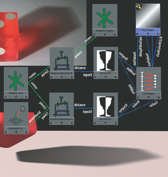
Figure 8.5. The diffuse quality of a depth map shadow is controlled by a Set Range utility. This scene is included on the CD as setrange_shadow.ma.
For the 3D render at the bottom of Figure 8.5, a directional light named Key is placed behind a polygon cube. The light's Use Depth Map Shadows attribute is checked. Two locators are placed in the scene. The first locator, named shadow_begin, is placed at a point on the ground where the shadow begins (close to the cube). A second locator, named shadow_end, is placed on the ground where the shadow ends.
Note
To accurately position a locator at the point where a shadow ends, select the shadow-casting light and choose Panels > Look Through Selected from a workspace view menu. The locator will be occluded by an object if it is within a shadow.
The center attribute of the shadow_begin transform node is connected to the point1 of a distanceBetween node (distanceBetweenB). The center of shadow_end is connected to point2 of distanceBetweenB. The Center attribute provides the location of an object's bounding box in world space. Ultimately, distanceBetweenB determines the length of the shadow. The center of shadow_end is also connected to the point2 of a second distanceBetween node (distanceBetweenA). The pointWorld attribute of a samplerInfo node is connected to the point1 of the distanceBetweenA. The Point World attribute stores the world position of the point being sampled during the render. Hence, distanceBetweenA determines the distance between the end of the shadow and the point being sampled. The distance of distanceBetweenA is connected to the inputX of a reverse node (reverseA). The outputX of the reverseA is connected to the valueX and valueY of a setRange node.
In the meantime, the distance of the distanceBetweenB node is connected to its own reverse node (reverseB). The outputX of reverseB is connected to oldMinX and oldMinY of the setRange node. The setRange node's MinX is set to 2 and its MaxX is set to 32. This represents the range of values that can be used as a Filter Size for the directional light. Since the Old Min value is fed by distanceBetweenB, and has been made negative by reverseB, the Old Max is set to 0. This negative range (–n to 0) matches the negative distance value provided by reverseA. These negative values are necessary to place the diffuse effect at the shadow end and not the shadow beginning. In this case, if a point near the end of the shadow is sampled, the distance between that point and the shadow_end is small and outputX of reverseA will be a small negative number (for example, −1). As a number, −1 is relatively high in the Old Min and Old Max range (close to 0) and is thus remapped to a number close to 32. Again, distanceBetweenB and reverseB represent the length of the shadow and therefore supply the Old Min values. If a point near the beginning of the shadow is sampled, the distance between that point and the shadow_end is large and outputX of reverseA will be a large negative number, such as −15. As a number, −15 is relatively low in the Old Min and Old Max range (not close to 0) and is thus remapped to a number close to 2.
Returning to the network, the outValueX of the setRange node is connected to the dmapFilterSize of the directional light KeyShape node. A dmapFilterSize of 0 produces no additional blur. A dmapFilterSize value of 32 creates the maximum amount of blur on the shadow. The outValueY of the setRange node is also connected to the shadColorR, shadColorG, and shadColorB of the light KeyShape node. The MinY of the setRange node is set to 0 and the MaxY is set to 0.5. This converts the Old Min and Old Max range into a range usable as a color. The end effect is a shadow that becomes lighter as it travels farther away from the cube. Increasing the value of MaxY will create a lighter shadow. This network works best with depth map shadows that have a relatively large Resolution value (for example, 1024). Smaller Resolution values will reveal the transitions between different Filter Size values. Nevertheless, this offers an alternative way to produce a diffuse shadow effect without the necessity of potentially time-consuming raytracing.
The Array Mapper utility is designed to control per-particle attributes on particle nodes. The attributes can affect particle size, dynamic behavior, color, and opacity. (An array is an ordered list of values.)
The simplest way to see the Array Mapper utility work is to create an RGB PP attribute for hardware-rendered particles. Since the process is a little unusual, I recommend you use the following steps:
Create a new scene. Switch to the Dynamics menu set and choose Particles > Create Emitter. Play back the Timeline. Select the resulting cloud of particles.
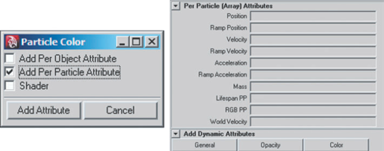
Open the Attribute Editor tab for a selected particle shape node (particleShape1) and expand the Lifespan Attributes section. Set the Lifespan Mode value to either Constant or Random Range and choose a Lifespan length (measured in seconds).
Click the Color button in the Add Dynamic Attributes section. The Particle Color window opens. Check the Add Per Particle Attribute option and click the Add Attribute button (see Figure 8.6). This adds an RGB PP attribute to the list in the Per Particle (Array) Attributes section of the particle shape node's Attribute Editor tab.
Right-click the field next to RGB PP and choose Create Ramp from the shortcut menu. A Particle Array utility and a Ramp texture are automatically connected to the particle shape node. The particles will then pick up the color of the ramp over their lifespan. You can render the default point particles with either the Maya Hardware renderer or the Hardware Render Buffer. (See Chapter 10 for more information on hardware rendering.)
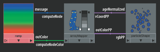
You can manually connect the Array Mapper utility (found in the General Utilities section of the Create Maya Nodes menu). For example, in Figure 8.7 the outColor of a ramp texture node is connected to the computeNodeColor of an arrayMapper node. The message of the ramp is also connected to the computeNode of the arrayMapper. The outColorPP of the arrayMapper node is connected to the rgbPP of the particleShape node. In turn, the ageNormalized of the particleShape node is connected to the vCoordPP of the arrayMapper node. The Min Value and Max Value attributes of the Array Mapper utility serve as a clamp for the outColorPP and outValuePP attributes (outValuePP is the single-attribute version of outColorPP). You can replace the ramp texture with other types of textures, but the results will be unpredictable.
Although color is used in the previous example, a number of other per-particle attributes are available, including incandescencePP, radiusPP, and opacityPP. You can access these attributes by clicking the General button in the Add Dynamics Attributes section of the particle shape's Attribute Editor tab and choosing the Particle tab of the Add Attribute: particleShape window (see Figure 8.8). In addition to the PP attributes, the Particle tab carries a long list of more esoteric attributes, any of which can be utilized for per-particle operations through an expression.
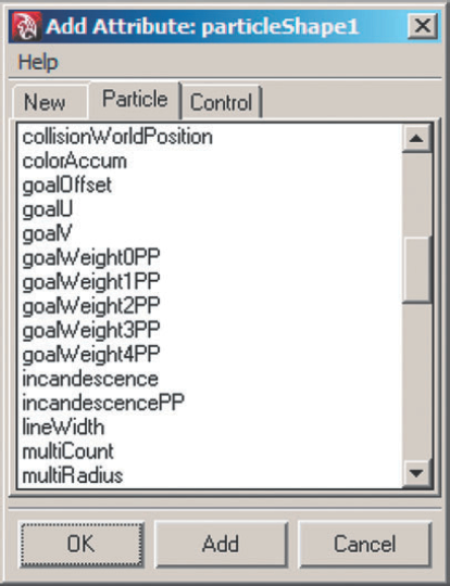
Figure 8.8. The Particle tab of the Add Attribute window. Only a small portion of the available PP attributes are shown.
In a second example, a single Array Mapper utility drives the color, opacity, and acceleration of a point particle node (see Figure 8.9).

Figure 8.9. A point particle node receives its color, opacity, and acceleration from an Array Mapper utility. This scene is included on the CD as array_point.ma. A QuickTime movie is included as array_point.mov.
To view the shading network, follow these steps:
With this network, the Noise attribute of the connected ramp node is set to 1 and its Noise Freq attribute is set to 50, which creates a random pattern throughout the ramp. Although rgbPP receives its color directly from the ramp node, an expression controls the particle node's opacity, acceleration, and lifespan. The expression follows:
particleShape.opacityPP=arrayMapper.outValuePP;
particleShape.acceleration=arrayMapper.outValuePP*-500;
particleShape.lifespanPP=rand(1,3);
To view the expression, follow these steps:
Choose Window > Animation Editors > Expression Editor.
Choose Select Filter > By Expression Name from the Expression Editor menu. Click the word particleShape in the Objects field.
Switch the Particles attribute to Creation. The expression code is revealed in the text field at the bottom of the window.
In the first line of the expression, outValuePP of the arrayMapper node drives opacityPP. In the second line of the expression, outValuePP drives the particle's acceleration attribute. The acceleration attribute controls the rate of velocity change on a per-particle basis (although it's not listed as a "PP"). You can see the effect of the variable acceleration if the particle count is reduced to a low number. Some particles move rapidly, while others fall very slowly. The outValuePP is multiplied by −500, which makes the acceleration more rapid and the particles' direction in the negative X, Y, and Z direction. The ability to use outValuePP as an input for multiple particle attributes eliminates the need for additional arrayMapper and ramp nodes.
In the third line of the expression, the particle lifespan is assigned a random number from 1 to 3 with the rand() function. The outValuePP attribute is automatically connected to input[0] of the arrayMapper node; this represents the use of outValuePP in an expression. When an expression is created for a per-particle attribute, the expression is carried by the particle shape node and no separate expression node is generated.
Note
Right-clicking an attribute field in the Per Particle (Array) Attributes section of a particle shape node's Attribute Editor tab provides the Creation Expression option in a shortcut menu. Creation Expression opens the Expression Editor and lists the particle shape and its numerous channels in the editor's Attributes list. Using the Creation Expression option is also a quick way to access preexisting per-particle expressions.
Creation expressions are executed at the start time of an animation. They are not executed as the animation plays. When using particles, a creation expression is applied one time per particle at the frame in which the particle is born. In contrast, a runtime expression executes at each frame during playback. A runtime expression is useful when values need to constantly change over the life of an animation. You can create a runtime expression by right-clicking an attribute field in the Per Particle (Array) Attributes section of a particle shape node's Attribute Editor tab and choosing Runtime Expression Before Dynamics or Runtime Expression After Dynamics.
As for other particle settings, the emitter is set to a cube volume shape with 0, −1, 0 Direction values. A turbulence field with a Magnitude value of 500 is also assigned to the particles. The field adds additional random motion; although the turbulence affects direction, it does not impact the overall acceleration. The end result is a glitter-like fall of particles. The point particles are rendered with the Hardware Render Buffer with Multi-Pass Rendering.
Unfortunately, the Array Mapper utility will not work with software-rendered particles—unless it is used in conjunction with a Particle Sampler utility. The Particle Sampler utility serves as a go-between, retrieving attribute information from a particle shape node and passing it on to a material assigned to the software-rendered particles. For example, in Figure 8.10 the example from Figure 8.9 is reused with the addition of a Particle Sampler utility. The Particle Render Type of the particle shape node is switched to Blobby Surface. The particle node is assigned to a blinn material node. The Noise value of the original ramp texture node is reduced and the ramp colors are adjusted. The Rate(Particles/Sec) value of the particle node is reduced for easier viewing. A directional light is added to the scene.
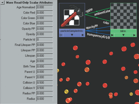
Figure 8.10. A Blobby Surface particle node receives its color, opacity, and acceleration through Array Mapper and Particle Sampler utilities. This scene is included on the CD as array_blobby.ma. A QuickTime movie is included as array_blobby.mov.
Aside from these adjustments, all the old network connections and the old expression are intact. As an addition, the rgbPP of a particleSamplerInfo node is connected to the color and the ambientColor of the blinn. The opacityPP of the particleSamplerInfo node is also connected to the transparencyR, transparencyG, and transparencyB of the blinn. The end result is a color distribution, opacity, lifespan, and acceleration roughly identical to Figure 8.9 but with a software-rendered particle node. The Particle Sampler utility also carries a long list of read-only attributes (see the left side of Figure 8.10). These attributes remotely read attribute information from the particle shape node that is assigned to the material. (For this to work, the material must share the shading network with the Particle Sampler utility.) The attributes are intuitively named (for example, particleSamplerInfo.rgbPP remotely reads particleShape.rgbPP). You can connect these attributes to any attribute of a material that may prove useful.
Note
You can change various per-particle attributes, such as lifespanPP and opacityPP, through the Particles tab of the Component Editor (Window > General Editors > Component Editor). You can select particle nodes in a workspace view by clicking the Select By Object Type: Dynamics button in the Status Line toolbar. You can select particles individually by clicking Select By Component Type: Points in the Status Line toolbar.
Note
Not all per-particle attributes will work with all particle render types. For instance, radiusPP will only work with Blobby Surface, Cloud, and Sphere particles. For a detailed attribute list, see "List of Particle Attributes" in the Maya help file.
Note
If particles are emitted from a NURBS or polygon object, they can derive their color from that surface. See the "Use a Texture to Color Emission or Scale the Rate" tutorial in the Maya help file.
Vectors are useful for determining direction within Maya. Matrices, on the other hand, are an intrinsic part of 3D and are necessary for converting various coordinate spaces. Comparing the direction of lights, cameras, and surface components within different coordinate spaces can provide information useful for custom shading networks. Before I discuss such networks, however, a review of vector math, the Vector Product utility, and Maya matrices is warranted.
In the mathematical realm, a vector is the quantity of an attribute that has direction as well as magnitude. For instance, wind can be represented by a vector since it has direction and speed (where speed is the magnitude).
In Maya, there are several variations of vectors. Vector attributes are simply a related group of three floating-point numbers. Color is stored as a vector attribute (R, G, B). At the same time, Maya vector attributes are used for transforms in 3D space. For instance, the translate of an object is represented as a vector attribute (X, Y, Z).
A second variation of a Maya vector is used to determine direction. That is, a particular point in space (X, Y, Z) has a measurable distance from the origin (0, 0, 0) and a specific angle relative to the origin. In this case, the distance serves as the vector magnitude and the angle is the vector direction. There are a number of specialized attributes that provide this style of vector (which can be loosely described as a "spatial vector"). A more detailed description of commonly used spatial vectors follows:
- Normal Camera and Surface Normal
The Normal Camera attribute is provided by the Sampler Info utility and material nodes. It represents the surface normal of the point being sampled in camera space. A surface normal is a vector that points directly away from the surface (and at a right angle to the surface). In general, surface normals are normalized so that their length (that is, their magnitude) is 1.
- Ray Direction
The Ray Direction attribute is provided by the Sampler Info utility and material nodes. It's a vector that runs from the surface point being sampled to the camera in camera space.
- Facing Ratio
The Facing Ratio attribute is uniquely provided by the Sampler Info utility and is the cosine of the angle between Ray Direction and Normal Camera. (A cosine is the trigonometric function often defined as the ratio of the length of the adjacent side to that of the hypotenuse in a right triangle.) The Facing Ratio is clamped between 0 and 1. A value of 0 indicates that the surface normal is pointing away from the camera. A value of 1 indicates that the surface normal is pointing toward the camera.
- Light Direction
The Light Direction attribute is provided by the Light Info utility and is a vector that represents the direction in which a light, camera, or other input node is pointing in world space. Lights also have a built-in Light Direction attribute (found in the Light Data section of the light shape node's Connection Editor attribute list). However, the Light Direction attribute of a light is in camera space.
The Vector Product utility accepts any vector attribute, whether it is a color, a transform, or a spatial vector. You can set the utility's Operation attribute to one of four modes:
- Dot Product
Dot Product multiplies two vectors together and returns a value that represents the angle between them. Its output may be written as
output= (a*d) + (b*e) + (c*f)The first input vector is (a, b, c) and is connected to Input 1 of the utility. The second input vector is (d, e, f) and is connected to Input 2 of the utility. The output is a single value. If Normalize Output is checked, the output is the actual cosine and will run between −1 and 1. −1 signifies that the vectors run in opposite directions. 0 signifies that the vectors are perpendicular to each other. 1 signifies that the vectors run in the same direction. When the Operation attribute is set to Dot Product, outputX, outputY, and outputZ attributes are the same value.
- Cross Product
Cross Product generates a third vector from two input vectors. The new vector will be at a right angle (perpendicular) to the input vectors.
- Vector Matrix Product and Point Matrix Product
Vector Matrix Product converts the coordinate space of a vector. This becomes useful when input vectors are in different coordinate spaces, such as camera and world. For conversion to work, the utility requires the connection of a transform matrix to its Matrix attribute. You can connect the XForm Matrix attribute of a camera or geometry transform node for this purpose. Xform Matrix is a world space matrix. Maya nodes also carry the World Matrix attribute, which is in world space. (For examples of shading networks using World Matrix, see Chapter 7.) The vector that requires conversion is connected to the Input 1 attribute. The Point Matrix Product operation offers the same space conversion, but operates on points.
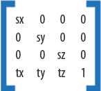
Maya uses a 4 × 4 matrix for transformations (see Figure 8.11). The position of an object is stored in the first three numbers of the last row. The object's scale is stored as a diagonal from the upper left. The object's rotation is indirectly stored within the first three vertical and horizontal positions from the upper-left corner; the rotation values are stored as sine and cosine values. When an object is created, or has the Freeze Transformations tool applied to it, its transform matrix is an identity matrix. An identity matrix is one that produces no change when it is multiplied by a second transform matrix. In other words, an object with an identity matrix has no translation, rotation, or increased/decreased scale.
As an example of camera space to world space conversion, in Figure 8.12 the Xform Matrix of a polygon cube is used to convert a Normal Camera vector of a Sampler Info utility into a world space vector. The results are illustrated by applying the resulting vector to the color of a material.
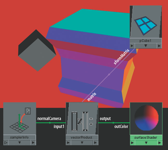
Figure 8.12. The Xform Matrix attribute of a polygon cube drives the color of a material. This scene is included on the CD as xform_matrix.ma. A QuickTime movie is included as xform_matrix.mov.
The xformMatrix of the pCube1 transform node is connected to the matrix of a vectorProduct node. (pCube1 is the small gray cube in Figure 8.12.) The normalCamera of a samplerInfo node is connected to the input1 of the vectorProduct node. The vectorProduct Operation value is set to Vector Matrix Product. The output of the vectorProduct node is connected directly to outColor of a surfaceShader material node, which is assigned to a second, larger polygon shape.
As a result of the custom connections, the faces of the larger shape that point toward the camera render blue until pCube1 is rotated. This is a result of the Normal Camera attribute existing in camera space. A normal that points directly toward the camera always has a vector of 0, 0, 1. At the same time, while pCube1 is at its rest position, its xformMatrix is an identity matrix and has no effect on the normalCamera value. Thus, the values 0, 0, 1 are passed to outColor of the surfaceShader node. When pCube1 is rotated, however, the normalCamera value is multiplied by the new xformMatrix and hence the color of the shape is affected. For instance, if pCube1 is rotated −45, −45, 0, a pale green results on the faces of the larger shape that point toward camera. The resulting math is illustrated in Figure 8.13.
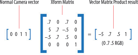
Figure 8.13. A matrix calculation based on pCube1's rotation of −45, −45, 0. The matrix numbers have been rounded off for easier viewing.
When representing the matrix calculation, as with Figure 8.13, the extra number 1 at the right side of the Normal Camera vector (and at the bottom-right corner of the Xform Matrix) is necessary for this type of math operation; however, these numbers do not change as the corresponding objects go through various transformations.
Note
As with many custom networks, the material icon in the Hypershade window, as well as the workspace view, may not provide an accurate representation of the material. To see the correct result for the previous example, use the Render View window.
Note
You can retrieve the current Xform Matrix value of a node by typing getAttr name_of_node.xformMatrix; in the Script Editor.
The Condition utility functions like a programming If Else statement. If Else statements are supported by Maya expressions and are written like so:
if ($test < 10){
     print "This Is True";
} else {
     print "This Is False";
}
If the $test variable is less than 10, Maya prints "This Is True" on the command line. The If Else statement serves as a switch of sorts, choosing one of several possible outcomes depending on the input. The function of the Condition utility, when written in the style of an If Else statement, would look like this:
if (First Term  Operation  Second Term){
     Color If True;
} else {
     Color If False;
}
First Term and Second Term attributes each accept a single input or value, while the Color If True and Color If False attributes accept vector values or inputs. The Operation attribute has six options: Equal, Not Equal, Greater Than, Less Than, Greater Or Equal, and Less Or Equal.
With the Condition utility, you can apply two different textures to a single surface. By default, all surfaces in Maya are double-sided but only carry a single UV texture space. Hence, a plane receives the same texture on the top and bottom. You can avoid this, however, with the shading network illustrated by Figure 8.14.
The flippedNormal of a samplerInfo node is connected to firstTerm of a condition node. The Flipped Normal attribute indicates the side of the surface that is renderable. If the attribute's value is 1, then the "flipped," or secondary, side is sampled. If the value is 0, the nonflipped, or primary, side is sampled. The nonflipped side is the side that is visible when the Double Sided attribute of the surface is unchecked.
Returning to the network, the outColor of a checker texture node is connected to the colorIfTrue of the condition node. The outColor of a file texture node is connected to the colorIfFalse attribute of the same condition node. A bitmap image of a hundred dollar bill is loaded into the file texture node. The condition's Second Term is set to 1 and Operation is set to Equal. Last, the outColor of the condition node is connected to the color of a blinn material node. Thus, the flipped side of a primitive plane receives the Checker texture while the nonflipped side receives the File texture.

Switch utilities provide multiple outputs from a single node. That is, they switch between different values in order to create different results among the geometry assigned to their shading network. Since the application of a Switch utility is unique in Maya, a step-by-step guide for a Triple Switch utility follows:
Choose an RGB attribute of a material, such as Color, and click its checkered Map button. Choose a Triple Switch from the Switch Utilities section in the Utilities tab of the Create Render Node window.
Assign the material to two or more surfaces.
Open the Attribute Editor tab for the tripleShadingSwitch node. Click the Add Surfaces button. All the surfaces assigned to the material appear in the list.
Right-click the first surface name in the Switch Attributes list and choose Map from the shortcut menu. The Create Render Node window opens. Choose a texture. The texture node appears in the Hypershade window. The Out Color attribute of the texture node (for example, stucco.outColor) appears in the inTriple column of the Switch Attributes list. Repeat this process for each of the remaining surfaces in the Switch Attributes list.
Render a test. Each surface picks up a different texture. An example is included as Figure 8.15.
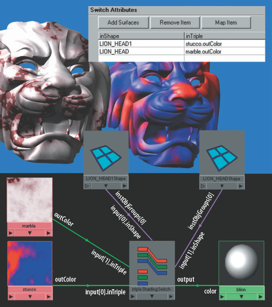
Although these steps apply the switch to a material, you can apply them to any node. That said, Triple Switches are designed for vector values and are best suited for any attribute that uses RGB colors or XYZ coordinates.
Single switches, on the other hand, are designed for scalar values and are best suited for such attributes as Diffuse, Eccentricity, Reflectivity, or Bump Value. The Single Switch utility automatically chooses the outAlpha attribute when a texture is chosen. In this case, the outAlpha of each texture connects to the input[n].inSingle of the singleShadingSwitch node. The n in input[n].inSingle corresponds to the slot number of the Switch Attributes list. The first slot is 0, the second is 1, and so on. Although geometry is also connected to the singleShadingSwitch node, the connection lines are initially hidden. Nevertheless, the instObjGroups[n] of each geometry shape node must be connected to the input[n].inShape of the singleShadingSwitch node. In this situation, the n of the instObjGroups[n] attribute refers to the hierarchy position of an instanced attribute. (See Chapter 7 for information on attribute instancing.) In most cases, n is 0. The instObjGroups[n] convention applies equally to Double, Triple, and Quad Switch utilities. In addition, all the switches possess variations of the input[n].inSingle input.
Double switches are designed for paired or double attributes. This makes the utility well suited for controlling UVs. For example, in Figure 8.16 a Cloth texture receives standard UV coordinates from a default place2dTexture node. The Repeat UV values, however, are supplied by a Double Switch utility. In this case, the repeatUV attributes of three additional place2dTexture nodes are connected to the input[n].inDouble attributes of the doubleShadingSwitch node. place2dTexture1 has a Repeat UV value of 5, 5. place2dTexture2 has a Repeat UV value of 25, 25. place2dTexture3 has a Repeat UV value of 50, 50. This shading network offers the ability to adjust UVs on multiple objects without affecting the base texture or necessitating the duplication of the entire shading network.
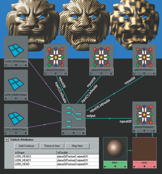
Figure 8.16. Repeat UV is controlled by a Double Switch utility. A simplified version of this scene is included on the CD as double_switch.ma.
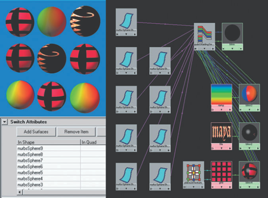
The Quad Switch utility is suited for handling a vector attribute and a single attribute simultaneously. For example, in Figure 8.17 the outTriple attribute of the quadShadingSwitch node is connected to the color of a blinn material node. The outSingle attribute of the quadShadingSwitch node is connected the diffuse of the same blinn. To split the switch's output in such a way, it is necessary to use the Connection Editor. The color attributes of three additional blinn nodes are connected to the input[n].inTriple attributes of the quadShadingSwitch node. The diffuse attributes of the blinn nodes are also connected to the input[n].inSingle attributes of the quadShadingSwitch node. Each of the three blinn nodes has the outColor of a different texture connected to their color and diffuse attributes. In this case, the diffuse attributes do not need to correspond with the color attributes. For instance, blinn2's color can be connected to input[0].inTriple and blinn2's diffuse can be connected to input[4].inSingle. This ability to mix and match outputs and inputs allows for a great diversity of results. Hence, the Quad Switch provides the flexibility necessary to texture crowds, flocks, and swarms. Although such custom connections will function properly, they do not appear in the Switch Attributes list of the switch's Attribute Editor tab.
Several utilities and nodes fail to fit into a specific category. Of these, the Stencil utility provides an alternative method of blending maps together. You can repurpose Optical FX and Unit Conversion utilities to fit a custom network. Although scene nodes (those automatically generated by Maya) are not particularly flexible, they provide critical services in a 3D scene.
As Stencil is the third texture application radio button listed in the 2D Textures section of the Create Maya Nodes menu (following Normal and As Projection). If a texture is chosen with As Stencil selected, the new texture automatically receives a Stencil utility and two place2dTexture nodes. The Stencil utility stencils the new texture on top of the material color. For example, in Figure 8.18 a red logo is applied to a wall map with this technique. Although the Stencil utility produces results similar to the Blend Colors utility (see Chapter 6), its methodology is fairly different.

Figure 8.18. A logo is applied to a wall with a Stencil utility. This scene is included as on the CD as stencil.ma.
In the example shading network, a red logo bitmap is loaded into a File texture named fileColor. The outColor of fileColor is connected to image of a stencil node. Standard UV connections run from the first place2dTexture node to fileColor. The second place2dTexture node is connected to the stencil node with similar (albeit fewer) standard UV connections. The outUV of the stencil's place2dTexture node is connected to the uvCoord of fileColor's place2dTexture node. The outUvFilterSize of the stencil's place2dTexture node is also connected to the uvFilterSize of fileColor's place2dTexture node.
Normally, this minimal set of connections will cause the fileColor texture to completely overtake the blinn's color. To avoid this, the outAlpha of a second file texture node, named fileMask, is connected to the mask of the stencil node. The Mask attribute controls where the new texture will show over the material color. In this case, a black and white bitmap is loaded into the fileMask node. Where the bitmap is white, the material color shows through; where the bitmap is black, the red logo is rendered.
At this point, the material color that is revealed by the Mask attribute can be only the solid color of the material's Color attribute. To avoid this, the outColor of a third file texture node, named fileWall, is connected to the defaultColor of the stencil node. In this example, a bitmap photo of a wall is loaded into the fileWall node. If fileWall was connected directly to the Color attribute of the blinn, it would not be visible.
The Optical FX utility (found in the Glow section of the Create Maya Nodes menu in the Hypershade window) is automatically created whenever Light Glow is applied to a directional, area, or spot light. The utility controls the look of the glow, halo, or lens flare. (For a discussion on this and other fog effects, see Chapter 2.)
Oddly enough, the Optical FX utility can be "grafted" onto a surface. For example, in Figure 8.19 the worldMatrix[0] attribute of a polygon lightbulb shape node is connected to the lightWorldMat of an opticalFX node. This connection ensures that the optical effect will occur in the center of the lightbulb regardless of the lightbulb's position. The color of the blinn node is connected to lightColor of the opticalFX node. The blinn Color attribute is set to gold, which is picked up by the opticalFX glow. (The lightbulb surface is also assigned to the blinn.) Last, the Ignore Light attribute of the opticalFX node is checked; this informs the program that no light is present. The result is a glow that follows the lightbulb wherever it goes. Unfortunately, since the opticalFX node creates a post-process effect, the size of the glow will not change. You can animate the Glow Spread and Halo Spread attributes of the opticalFX node, however, if necessary.

The Unit Conversion node, while not accessible in the Create Maya Nodes menu, automatically appears in many custom networks. For example, in Figure 8.20 the translateX of a cone transform node is connected to the rotateX of a sphere transform node. To view the connection, follow these steps:
Open
unit_conversion.mafile from the CD. Select the sphere and cone. Choose Window > Hypergraph: Connections.Choose Show > Show Auxiliary Nodes from the Hypergraph Connections menu (so that the option is checked). A unit conversion node should appear between the sphere and cone transform nodes.
If the node fails to appear, choose Show > Auxiliary Nodes from the Hypergraph Connections menu. In the Auxiliary Nodes window, highlight the word unitConversion in the Node Types That Are Hidden In Editors field and click the Remove From List button.
Alternatively, if you MMB-drag the sphere or cone transform node into the Hypershade work area, clicking the Input And Output Connections button reveals the unit conversion node.
By default, Maya calculates the translation of objects using Linear working units. At the same time, Maya calculates the rotation of objects using Angular working units. Whenever two dissimilar working units, such as Linear and Angular, are used in the same network, Maya must employ a Unit Conversion node to create accurate calculations. In the example illustrated in Figure 8.20, a Unit Conversion node is automatically provided with a Conversion Factor attribute set to 0.017. You can change Conversion Factor to achieve an exaggerated effect. If the Conversion Factor attribute is changed to 1, for example, the sphere will spin at a much greater speed when the cone is transformed.
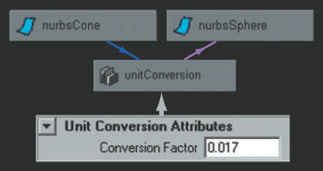
Figure 8.20. A Unit Conversion node converts two dissimilar units of measure. The scene is included on the CD as unit_conversion.ma.
Note
You can set a scene's working units by choosing Window > Settings/Preferences > Preferences and switching to the Settings section of the Preferences window. The default Linear working unit is centimeters and the default Angular working unit is degrees.
Note
In general, it's best to work in inches or centimeters. On occasion, calculation errors occur if a scene is set to meter, foot, or yard Linear units. For example, a scene set to foot units can exceed the maximum unit limit of a camera clipping plane and objects will fail to fully draw in the camera view.
Render Partition, Default Light Set, and Light Linker nodes sit the farthest downstream in any shading network (see Figure 8.21). The Render Partition utility defines which shading group nodes are called upon during a render.
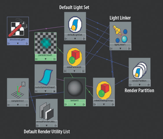
The Default Light Set utility carries a list of lights that illuminate all objects within a scene. The instObjGroups[0] attribute of each light's transform shape node is connected automatically to the dagSetMembers[0] attribute of the defaultLightSet node. If you uncheck the Illuminates By Default attribute in a light's Attribute Editor tab, the connection is removed until the attribute is once again checked.
The message of the defaultLightSet node is connected automatically to link[n].light and shadowLink[n].shadowLight of the lightLinker utility node. The Light Linker utility defines the relationship between lights and objects. If a light is connected through to defaultLightSet node to the link[n].light attribute, the light illuminates all shading groups connected to the lightLinker node. If a light is connected through the defaultLightSet node to the shadowLink[n].shadowLight attribute, then the light creates shadows for all shading groups connected to the lightLinker node. All shading group nodes are connected automatically to the lightLinker node. However, if you manually delete the connections, the shading group and the shading group's materials are ignored by the lights in the scene.
The Light Linker utility also stores broken links between lights, shadows, and surfaces. If a light link is broken through the Break Light Links tools, a connection is made between the message attribute of the surface shape node to the ignore[n].objectIgnored of the lightLinker node. A connection is also made between the message of the light shape node and ignore[n].lightIgnored of the lightLinker node. If the Make Light Links tool is applied, the connections are removed. Similar connections are made between the surface and light shape nodes' message and the lightLinker node when the Break Shadow Links tool is applied.
If a light is linked or unlinked in the Relationship Editor, the connections are identical to those made with the Make Light Links and Break Light Links tools. For more information on the Relationship Editor, Make Light Links, and Break Light Links, see Chapter 2.
The Default Render Utility List node holds a list of all render utilities in Maya. Although it cannot be used for any other purpose, it will show up in custom shading networks connected to each and every utility node.
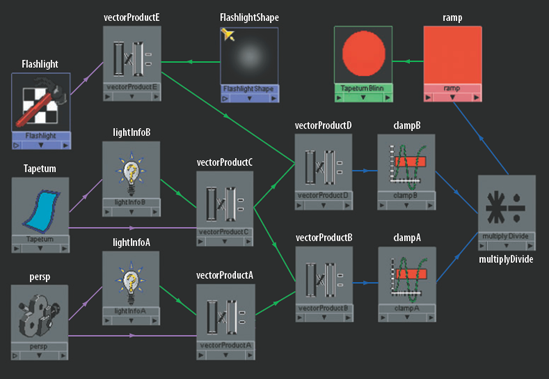
In this section, you will re-create the tapetum lucidum of an eyeball. The tapetum lucidum is a highly reflective membrane behind or within the cornea of many mammals and is responsible for the creepy eye glow seen at night. (Although a similar effect occurs when a flash photograph creates "red eye," humans don't possess the membrane.) You will use Light Info, Vector Product, and Multiply Divide utilities, as well as a Ramp texture. The tapetum lucidum of the eyeball geometry will become bright red only when both the camera and the scene's spot light are pointing directly toward it (see Figure 8.22).
Open
tapetum.mafrom the Chapter 8 scene folder on the CD. This file contains an eyeball model. A NURBS disc, which sits behind the iris, is named Tapetum and will provide the tapetum lucidum effect. A spot light, named Flashlight, is placed near the eye. It will serve as the scene's single light source and will figure into the calculations.MMB-drag two Light Info utilities into the Hypershade work area. Name the first lightInfoA and the second lightInfoB. Switch over to the Lights tab of the Hypershade window and MMB-drag the FlashlightShape node into the work area.
Open the Hypergraph window. MMB-drag the persp camera transform node, the Flashlight transform node, and the Tapetum geometry transform node into the Hypershade work area. Connect worldMatrix[0] of the camera transform node to the worldMatrix of lightInfoA. Connect the worldMatrix[0] of the Tapetum geometry transform node to worldMatrix of lightInfoB.
MMB-drag five Vector Product utilities into the work area. Name the first vectorProductA, the second vectorProductB, the third vectorProductC, the fourth vectorProductD, and the fifth vectorProductE. See Figure 8.23 for the placement of the nodes.
Connect lightDirection of the FlashlightShape node to input1 of vectorProductE. (The Light Direction attribute is listed within the Light Data section of the light shape node's attribute list when the node is loaded into the Connection Editor.) Connect xformMatrix of the Flashlight transform node to matrix of vectorProductE. Set vectorProductE's Operation to Vector Matrix Product and check Normalize Output. This will convert the lightDirection vector into a usable world space vector.
Connect xformMatrix of the Tapetum transform node to matrix of vectorProductC. Connect lightDirection of lightInfoB to input1 of vectorProductC. Set vectorProductC's Operation to Vector Matrix Product and check Normalize Output. This will convert the direction of the Tapetum geometry into a usable world space vector.
Connect xformMatrix of the persp camera transform node to matrix of vectorProductA. Connect lightDirection of lightInfoA to input1 of vectorProductA. Set vectorProductA's Operation to Vector Matrix Product and check on the Normalize Output button. This will convert the camera direction into a usable world space vector.
Connect output of vectorProductC to input2 of vectorProductB. Connect output of vectorProductA to input1 of vectorProductB. Set vectorProductB's Operation to Dot Product and check Normalize Output. This will calculate the angle between the Tapetum geometry direction and the persp camera direction.
Connect output of vectorProductC to input2 of vectorProductD. Connect output of vectorProductE to input1 of vectorProductD. Set vectorProductD's Operation to Dot Product and check Normalize Output. This will calculate the angle between the Tapetum geometry direction and the flashlight light direction.
MMB-drag two Clamp utilities into the work area. Rename them clampA and clampB. Connect outputX of vectorProductB to inputR of clampA. Connect outputX of vectorProductD to inputR of clampB. For each clamp node, set MinR to 0 and MaxR to 1. This will prevent any negative numbers from reaching the end of the shading network.
MMB-drag a Multiply Divide utility into the work area. Connect outputR of clampA to input1X of the multiplyDivide node. Connect outputR of clampB to input2X of the multiplyDivide node.
Set the multiplyDivide Operation to Multiply. If the Flashlight points toward the eye, input2X becomes roughly 1. If the eye is "looking" at the camera, input1X also becomes 1. In this the case, the surface normals of the Tapetum are pointing down the negative Z axis, whereby they are actually pointing in the same direction as the camera (you can see this if the Double Sided attribute is unchecked for the surface). If the eye is "looking" away, input1X becomes roughly 0. Similarly, if the light points 90 degrees away from the eye, input2X becomes 0. Hence, when the eye points toward the camera and the light points toward the eye, the multiplyDivide node outputs a large value. If either the camera or the light points away from the eye, the output value becomes smaller. Only the angles of the light, camera, and geometry are compared. Although object position is part of the Xform Matrix attribute, the position of the object does not affect the output of the Dot Product operation. In other words, the light might produce a normalized cosine of 0.5 whether it's positioned at 0, 0, 0 or 500, 500, 500.
MMB-drag a Ramp texture and a Blinn material into the work area. Connect the outputX of the multiplyDivide node to vCoord of the ramp node. Create two handles in the ramp color field, one red and one black. Place the black handle at a Selected Position value of 0.75 and the red handle at a Selected Position value of 1. The ramp should have a thin red strip at the top with the bulk of the color black. Set the ramp's Interpolation attribute to Smooth. Connect outColor of the ramp node to incandescence of the blinn node. Assign the blinn to the Tapetum geometry.
Select the iris, cornea, and eyewhite geometry and parent them to the Tapetum. The vector calculations will only be accurate if the Tapetum geometry is at the top of the eye hierarchy.
The custom shading network is complete! Render out a few tests. No matter where the camera is, if the eye points toward it and the light points toward the eye, the tapetum lucidum will become bright red. If you get stuck, the finished scene is saved as
tapetum_finished.main the Chapter 8 scene folder.