Although the Hypershade window provides numerous ways to prepare materials, several important techniques outside the window are worth a look. Preparing proper UVs for any model is a critical step in the texturing process. Using the 3D Paint tool is an efficient way to prepare custom bitmaps. Maya's support of the Photoshop PSD format allows the use of layers. At the same time, the proper use of bump and displacement maps can add realism to a render. Last, custom sliders can automate a material.
Chapter Contents
UV approaches for NURBS and polygon surfaces
Tips and tricks for fixing UV problems
Workflow for the 3D Paint tool
Support of the Photoshop PSD format
Intricacies of bump and displacement maps
Creating custom sliders for materials
The NURBS and polygon surfaces employed in the examples featured by previous chapters carry UV texture spaces that are satisfactory for their corresponding renders. For a render to be successful, the UV texture space of a surface must avoid undue stretching, pinching, or overlapping. Although the modeling steps necessary to create high-quality UVs are numerous and beyond the scope of this book, a few important concepts and techniques are worth reviewing.
To display the UV texture space of a selected surface, choose Window > UV Texture Editor. By default, U runs from left to right; V runs from bottom to top. In the UV Texture Editor, the dark gray area in the upper-right portion of the grid represents the full UV texture space. If a face sits outside this area, it will receive a repeated portion of a texture. UV manipulation of polygon, subdivision, and NURBS surfaces differs greatly. Techniques for dealing with each surface type follow.
Note
UV texture space is a coordinate space that relates pixels of a texture to points on a surface. UV points represent the location of a polygon's vertices within UV texture space; you can transform UV points in the UV Texture Editor. Groups of connected UV points are known as UV shells. UVs is a loose term for the current state of UV points in a particular UV texture space.
NURBS surfaces automatically receive UV texture information when they are created. 0, 0 in UV texture space occurs at the origin box of the surface. The two vertices appearing closest to the origin box are represented by a tiny U and V, indicating the U and V direction (see Figure 9.1).

In general, NURBS surfaces are ready to texture as soon as they're created. Nevertheless, an understanding of parameterization, closed and periodic surfaces, stretching, and UV alignment will strengthen your texturing skills.
NURBS surfaces are inherently parametric. In general terms, parameterization is the mapping of one domain to a second domain. For example, the Earth, as a spherical planet, is mapped to rectangular travel maps. In terms of NURBS surfaces, parameterization is the method by which values are assigned to curve parameters. Curve parameters are points along the length of a curve or surface that have unique values. As the points get farther away from the origin of the curve or surface, their values increase. The parameter range of a NURBS primitive plane is 0 to 1. The parameter range of other NURBS primitives and custom NURBS surfaces is 0 to the total number of surface spans, which run from edit point to edit point. Ultimately, the parameter points determine the UV value of any given point on the corresponding surface. By default, NURBS surfaces automatically fill the entire UV texture space (see Figure 9.2). Regardless of the surface parameter range, the UV Texture Editor always displays a normalized UV range of 0 to 1.

You can apply parameterization in Maya using two methods: uniform and chord length. The uniform method assigns parameter values to each edit point. The assignment does not take into account the length of any given span; instead, the uniform method only considers the total number of spans. Thus, if a curve has four edit points and three spans, the edit points will have the values 0, 1, 2, and 3 (see Figure 9.3). The uniform method is efficient and easy to visualize. However, its interpolation is not as accurate as the chord length method and can lead to unpredictable texture stretching.

Figure 9.3. Uniform and chord length parameter values on similar curves. These curves are included on the CD as uniform_chord.ma.
Technically, chord length is the shortest linear distance between successive edit points. Chord length parameterization assigns parameter values based on these measurements. In other words, the parameter values are distributed unevenly along the curve and are not intrinsically bound to the number of edit points or spans (see Figure 9.3). The parameter values are based on world units and tend to be fairly large. The chord length method is more accurate but is difficult to visualize and predict. Surfaces based on chord length curves can be more complex and potentially flawed. (For example, they can suffer from the addition of extra isoparms, which is known as cross-knot insertion.)
By default, the CV Curve tool creates uniform curves. However, you can create chord length curves by choosing Create > CV Curve Tool >
Note
To normalize the parameter range of a curve, switch to the Surfaces menu set, choose Edit Curves > Rebuild Curve >
Note
You can observe the parameter values of uniform and chord length curves, as well as NURBS surfaces, by displaying their edit points and clicking the curve or surface isoparm. The Script Editor displays select -r curve_name.u[parameter_value]; or select -r surface_name.uv[u_parameter][v_ parameter];.
Texture stretching on NURBS surfaces is generally caused by one of the following reasons:
An uneven distribution of surface isoparms exists due to unevenly spaced curves at the point of surface creation.
Open/Close Surfaces or Attach Surfaces tools have been applied to the surface.
Vertices have been moved a significant distance from their neighboring vertices.
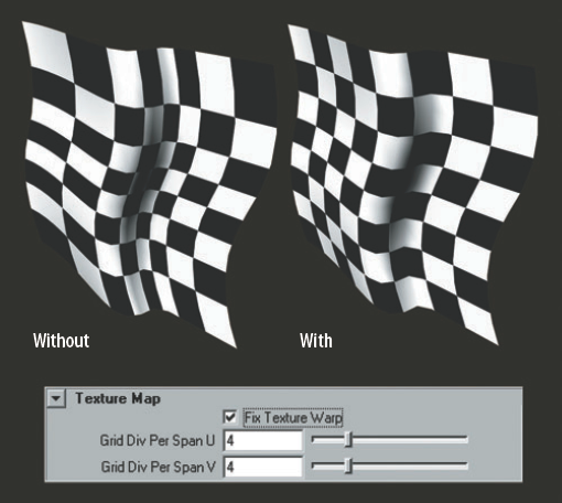
You can temporarily fix texture stretching by checking the Fix Texture Warp attribute found in the Texture Map section on the surface's Attribute Editor tab (see Figure 9.4). In this case, the renderer ignores the inherent UV information of the surface and applies a new, nonpermanent chord length parameterization. The Grid Div Per Span U and Grid Div Per Span V attributes set the density of a virtual grid that is placed over the surface to calculate the new UV texture space. Although the default value of 4 works in most situations, you can increase the value for greater accuracy. This fix is supported by the Maya Software and mental ray renderers but will not work with the Hardware Texturing option in a workspace view.
A second solution involves a "quick and dirty" method of reconstructing the surface. Using the stretched_surface.ma file in the Chapter 9 scene folder of the CD, you can follow these three steps:
While pressing the Shift key, insert evenly distributed isoparms across the surface in the direction of the stretching. The greater the number of isoparms, the more accurate the end product will be. Shift-select the two end isoparms. Use Figure 9.5 as a reference for each step.
With the new isoparms and the end isoparms selected, switch to the Surfaces menu set and choose Edit Curves > Duplicate Surface Curves. New curves will appear at all the isoparm locations. Delete the original surface.
Select the new curves in logical order (for example, left to right). Choose Surfaces > Loft with the default settings. Delete the curves. The final surface will have an evenly distributed UV texture space (at least in the direction of the loft).

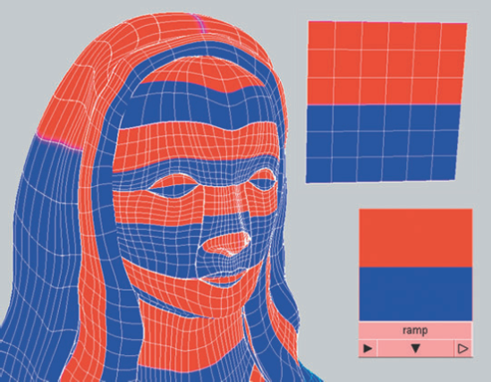
To create a complex model with NURBS modeling tools, multiple surfaces are necessary. In this situation, it is important to align the UVs in such a way that they are easily interpreted. One technique employed professionally involves a global alignment of all the surfaces. For example, in Figure 9.6 a character is constructed from numerous NURBS surfaces. A Ramp texture is temporarily assigned to each surface, and Smooth Shade All and Hardware Texturing are checked through a workspace view menu. If the orientation of the ramp on a given surface matches the orientation of the ramp's material icon, the UVs are correctly aligned. That is, U runs left to right and V runs down to up. If a ramp appears sideways or upside down on a surface, you can fix the UVs by switching to the Surfaces menu set and choosing Edit NURBS > Reverse Surface Direction. To choose the correct option on the Reverse Surface Direction tool, it is important to understand the relationship of the NURBS surface normal to the U and V directions.
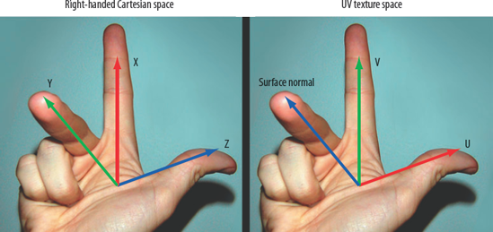
If U runs left to right and V runs down to up, the normal points toward the camera. If U runs right to left and V runs down to up, the normal points away from the camera. If U is running up and down and V is running left and right, the ramp will appear sideways. One way to remember this is to employ a variation of the right-handed Cartesian coordinate trick. Normally, in right-handed Maya coordinate space, the thumb points toward positive Z, the middle finger points toward positive Y, and the index finger points toward positive X. With a Maya NURBS surface, the thumb points toward positive U, the index finger points toward positive V, and the middle finger represents the direction of the surface normal (see Figure 9.7). All surfaces in Maya are double-sided by default. If the Double Sided attribute is unchecked in the Render Stats section of the surface's Attribute Editor tab, the UV-to-normal relationship is easier to see.
Note
Some animated productions require that all NURBS surfaces remain single-sided. A quick way to "flip" the normal of any single-sided surface that is pointing away from the camera is to switch to the Surfaces menu set, choose Edit NURBS > Reverse Surface Direction >
Although NURBS surfaces are ready to render with their default UVs, polygon surfaces often need a great deal of adjustment. The use of primitives is the exception since the primitive's inherent UVs are orderly. As soon as various polygon modeling tools are applied to a primitive, however, the resulting UV texture space is cluttered and unusable (see Figure 9.8).

There are two main approaches to preparing UVs within Maya: pelt mapping and mapping tools. Pelt mapping generally requires a specialized MEL script, but can be achieved with standard UV tools through the UV Texture Editor. Mapping tools, on the other hand, are built into the program and represent the most common method of UV preparation.
Pelt mapping unwraps geometry as if it were the pelt or skin of an animal. The goal with this approach is to create a single, large UV shell for the entire surface. This simplifies the texturing process by minimizing the number of resulting edges. In addition, the pelt mapping process creates a UV point distribution that mimics the original mesh. That is, the distance between each point is equivalent to the distance between matching vertices.
Several MEL scripts automate the creation of pelt mapping. For example, pelt.mel, available at http://highend3d.com, operates in the following manner:
Creates a duplicate of the target surface.
Allows you to define seams on the duplicate by cutting edges.
Creates control clusters for each cut and attaches specialized particles, springs, and radial fields to each vertex.
Sends the duplicate through a dynamic simulation complete with gravity. A collision plane is provided to "catch" the flattened duplicate.
Transfers vertex positions from the flattened duplicate to the UV texture space of the original surface. Thus, vertex postions become UV points.
The most difficult aspect of this pelting method is the selection seams. Ultimately, the goal is to create an unfolded, nonoverlapping surface that fits neatly into the UV texture space. As an example of pelt.mel in action, a polygon ear is flattened (see Figure 9.9).

Figure 9.9. (Clockwise, from upper left) A duplicate ear awaits the dynamic simulation provided by pelt.mel; the ear dynamically unfolds; the final UV texture space; the UV texture space prior to the operation.
Pelting Tools, available at http://hydralab.com, uses a methodology similar to pelt.mel. It offers the advantage, however, of interactive tools to define seams and a graphic interface with a greater number of options (see Figure 9.10).
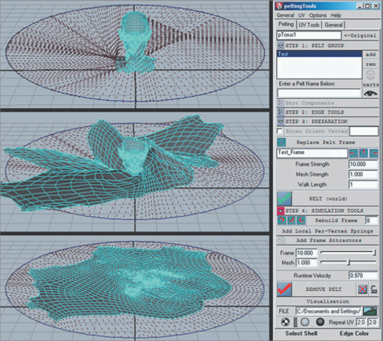
Figure 9.10. (Left) A polygon head goes through a dynamic unfolding. (Right) GUI for Pelting Tools MEL script. A QuickTime movie showing the unfolding is included on the CD as head_pelt.mov.
You can also create pelt maps in Maya with the standard set of UV tools. For example, in Figure 9.11 the UV points for the body of a polygon dog are left in one continuous piece. In this case, multiple UV mappings were applied to various parts of the dog. The resulting UV shells were then translated, rotated, scaled, and sewn back together with the Sew UV Edges and Move And Sew UV Edges tools.

You can find UV mapping tools under the Create UVs menu in the Polygons menu set. The mapping tools include Planar Mapping, Cylindrical Mapping, Spherical Mapping, and Automatic Mapping. To apply a mapping tool, select a polygon surface or set of faces and choose the tool. For example, in Figure 9.12 the Cylindrical Mapping tool is applied to a polygon primitive helix. A projection manipulator instantly appears. You can interactively adjust the sweep, height, translation, and rotation of the manipulator by clicking the various colored handles. The green boxes adjust projection height. The red boxes increase or decrease the horizontal sweep (by default, the cylindrical projection only covers 180 degrees). To access the rotation and translation handles, click the red T and the bottom of the manipulator. As the manipulator is adjusted, the UV points automatically update in the UV Texture Editor (Window > UV Texture Editor).
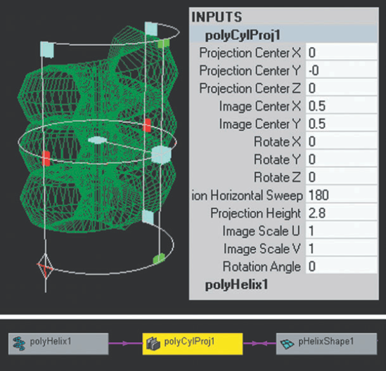
Figure 9.12. (Top left) Cylindrical Mapping projection manipulator applied to a polygon helix. (Top right) The polyCylProj1 node in the Channel Box. (Bottom) The polyCylProj1 node in the Hypergraph Connections window.
Here are a few additional tips for working with mapping tools and their projection manipulators:
- Projection Manipulator
The manipulator provided by all polygon UV mapping tools is finicky and tends to disappear when a mouse click is slightly off. Fortunately, you can bring back the manipulator by selecting the projection node. You can find the projection node in the Hypergraph Connections window (see Figure 9.12). You can also retrieve the manipulator by selecting the surface and opening the Channel Box. The projection node will be listed under Inputs (see Figure 9.12). For example, a Cylindrical Mapping projection node will be named polyCylProj1. Clicking the projection node name reveals the projection's attributes and displays the manipulator in the workspace view. If interactive use of the manipulator proves impossible, you can set the projection node's Projection Horizontal Sweep, Projection Height, Rotate, and other projection-specific attributes in the Channel Box. The projection node will remain connected to the surface shape and transform nodes until the surface's history is deleted. At the point of deletion, the UV information is permanently encoded.
Note
Although it is possible to overlap mapping tool projections, it is not recommended. Multiple, active, overlapping projections can lead to flickering textures. If multiple, overlapping projections are deemed necessary, delete the surface's history (Edit > Delete By Type > History) between applications of each mapping. Active mapping tool projections on a skinned, deforming character are equally problematic.
- Multiple Projections
You can apply UV mapping tools to entire polygon surfaces or to selected faces. On complex models, it often pays to apply separate mappings to various sections; at the same time, it is useful to have all the UV points in a single layout. For instance, if the model is a character, the head is mapped first, then the torso, then one arm, then the next, and so on. This allows different mapping styles and orientations to be applied. For example, the Cylindrical Mapping tool is applied to the head along the Y axis. The Cylindrical Mapping tool is applied a second time to an arm along the X axis. Separate Planar Mapping tools are applied to each hand. To replicate this process efficiently, follow these steps:
Select a set of faces. Apply the most appropriate mapping tool. Open the UV Texture Editor. If the projection manipulator is visible in the workspace view, a corresponding translate, scale, and rotate handle is accessible in the UV Texture Editor. Move the selected UV points into an empty area outside the gray area of the full UV texture space (see Figure 9.13). When the UV points are deselected, the entire surface becomes visible once again. The mapping separates the selected faces along the outer edges. (A group of separated UV points is called a UV shell.) If possible, separate the model at a natural border to avoid visible texture seams (for example, between a shirt collar and a neck).
Repeat the process for other sets of faces. Once all the faces have been mapped, move, scale, and rotate the individual UV shells back into the gray area.
To see how faces have been split in the UV Texture Editor, right-click and choose Edge from the marking menu. Click an outer edge of an UV shell. The corresponding edge that was separated during the mapping process is highlighted.
Although no technical problems will arise from separated faces, the separation can make the texturing process more difficult. To avoid this, you can sew selected faces back together (for example, reattaching a neck and a head). To do this, select one or more edges and choose Polygons > Sew UV Edges in the UV Texture Editor window. The faces that were once separated are rejoined. Sew UV Edges moves the resulting sewn edge to a point halfway between the previously separated faces (see Figure 9.14). This may or may not be useful. An alternative is to choose Polygons > Move And Sew UV Edges, which forces all the faces connected to the selected edge to move up to the second selected edge (see Figure 9.14). Move And Sew UV Edges does not prevent overlapping. If you need to manually split an edge, select the edge and choose Polygons > Cut UV Edges.

Ideally, UV points should maximize the UV texture space without overlapping. The amount of space dedicated to each section of a model should be relative to that section's importance. In addition, distances between UV points should be roughly equivalent to the distances between the vertices that they correspond to. That is, if vertices on the model are regularly spaced, the UV points should also be regularly spaced. If the vertices on the model are closer together in the Y direction than they are in the X direction, the UV points should be closer together in the V direction than they are in U direction.
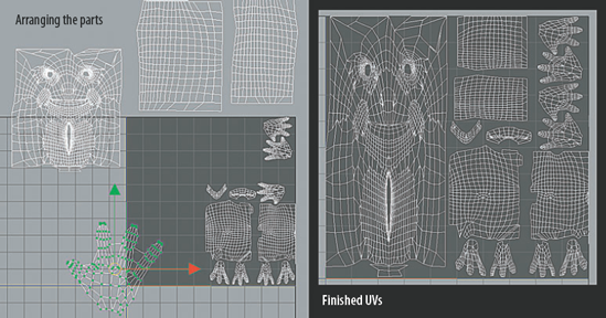
These guidelines are particularly critical for models intended for the video game industry, where textures are hand-painted and the texture resolutions are limited. For example, in Figure 9.15 a low-polygon character and a matching color bitmap are carefully laid out. Ideally, there should be a minimal amount of empty space left between the various UV shells.

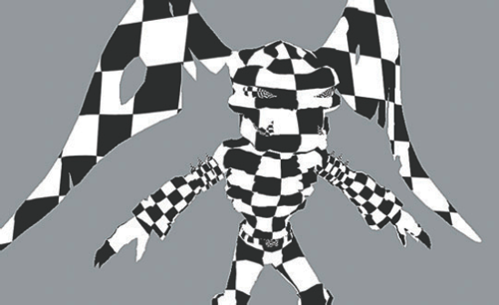
A good way to test UVs for potential stretching, pinching, or overlapping problems is to temporarily assign a Checker texture to the surface and choose Shading > Hardware Texturing from a workspace view menu (see Figure 9.16). Once an error has been located or a refinement planned, you can utilize a long list of Maya UV tools. These tools are available through the Polygons menu in the UV Texture Editor window or through the Edit UVs menu found in the Polygons menu set. A few of the more useful UV tools are highlighted in the following sections.
You can select UV points in the UV Texture Editor by right-clicking and choosing UV from the marking menu. Once selected, UV points can be translated, scaled, and rotated with standard Maya transform tools.
Choosing Polygons > Normalize in the UV Texture Editor fits the entire surface (or selected points, edges, or faces) into the full UV texture space. This ensures that a higher percentage of the UV texture space is utilized.
One inherent danger of the Normalize tool is the tool's inability to compensate for "stranded" points. Stranding is an artifact of the Cylindrical Mapping and Spherical Mapping tools (see Figure 9.17). If points are stranded, it's best to manually move them back to the main shell before applying Normalize.

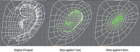
Choosing Polygons > Relax in the UV Texture Editor spreads out overlapping and/or high-density clusters of selected UV points. For example, in Figure 9.18 a polygon ear has the Relax tool, with default settings, applied to it multiple times. Parts of the model that were once overlapping are flattened out.
The following options can improve the quality of the relaxation:
- Edge Weights
If set to World Space, Edge Weights attempts to maintain the original world space angles between faces. If left on Uniform, Edge Weights attempts to make all the edges the same length. Uniform produces a more drastic relaxation than World Space.
- Pin UVs and Pin UV Border
If Pin UVs is checked, Pin Selected UVs and Pin Unselected UVs options become available. If Pin Selected UVs is then checked, selected UV points will stay in place and unselected UV points will move as they are relaxed. If Pin Unselected UVs is checked instead, the opposite occurs. If Pin UV Border is checked, the outer edges of the UV shell will remain fixed while the rest of the UV points will move. You can check both Pin UVs and Pin UV Border for a more refined result.
- Maximum Iterations
Sets the number of iterations permitted to the relaxation calculation each time the tool is applied. The lower the value, the more subtle the resulting relaxation. The higher the value, the more extreme the relaxation.
Note
If the vertices at the shared corner of multiple polygon faces have not been merged, the Relax tool will open a hole in the geometry.
Choosing Polygons > Layout in the UV Texture Editor automatically arranges UV shells within the UV texture space. For relatively simple models, the resulting arrangement is neat and orderly. The Layout tool will even work across multiple surfaces. (To prevent overlapping, set Layout Multiple Objects to Non-Overlapping.) Since the tool leaves a significant amount of empty space, additional manipulation of the UV points may be required (see Figure 9.19).

The creation of UV sets allows a single surface to carry multiple UV layouts. A UV layout is simply a unique arrangement of UV points. Since overlapping is not an issue for UV sets, each UV set and corresponding UV layout can cover the entire UV texture space. Without the use of UV sets, you must carefully arrange individual UV shells belonging to a single surface within the UV texture space (as demonstrated in Figure 9.13 earlier in this chapter). As an additional benefit, each UV set can support a unique UV layout even when polygon faces within the set belong to multiple UV sets. Ultimately, you can assign each UV set to a different texture, thus allowing for a more complex and advanced texturing approach.
To create a UV set during the UV mapping process, open the Options window for the Planar Mapping, Cylindrical Mapping, Spherical Mapping, or Automatic Mapping tool. Check Create New UV Set, enter a name in the UV Set Name field, and click Apply. Once UV sets exist, you can view them, one at a time, in the UV Texture Editor by selecting the surface and choosing UV Sets > UV_Set_Name (see Figure 9.20).
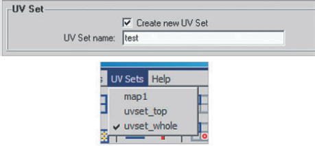
Figure 9.20. (Top) The Create New UV Set attribute within the Planar Mapping Options window. (Bottom) The UV Sets menu in the UV Texture Editor.
In addition, you can create new UV sets in the UV Texture Editor at any time. To do this, select a series of UV points, edges, or faces and choose Polygons > Copy UVs To UV Set > Copy Into New UV Set >
You can link UV sets to specific textures by following these steps:
Create several UV sets for a surface. Assign the surface to a material that has several textures mapped to it. For example, assign the surface to a Blinn material with a File mapped to its Color and a Noise mapped to its Specular Roll Off.
Choose Window > Relationship Editors > UV Linking > UV-Centric. The Relationship Editor window opens. Initially, the UV Sets and Textures columns are empty. Select the surface in a workspace view. The surface, with its UV sets, is listed in the left column. The assigned material, with its texture maps, is listed in the right column.
Click the map1 UV set name in the left column. The map1 UV set is the default UV set that contains all the UV points of the surface. The textures that the map1 set are linked to are highlighted in the right column of with a gray bar. You cannot directly disable the texture links to the map1 UV set.
Click a custom UV set name in the left column. The textures listed in the right column remain unhighlighted, which indicates that there is no texture link. Render a test frame. At this point, the render is standard and does not employ the custom UV sets for the selection of textures.
Click a texture name in the right column. A link to the UV set is created. Click the map1 UV set name. Note that the texture linked to the custom UV set is now unlinked for the map1 UV set. The texture cannot be linked to the map1 set and the custom set at the same time. Render a test. The texture that is linked to the custom UV set appears only on those faces that belong to the custom UV set.
You can link a texture to one UV set at a time. If you wish to have the texture linked to all the UV points, and faces, of a surface, reestablish the link between the texture and the map1 UV set. To reestablish a link, simply click the texture name so that it is highlighted with a gray bar. You can link a UV set to more than one texture. When a link is made between a texture and a custom UV set, a uvChooser utility node is connected automatically to the place2dTexture node that belongs to the texture.
As an example, in Figure 9.21 two UV mappings are applied to a polygon primitive shape. The Planar Mapping tool is applied to the topmost faces and receives a UV set named uvset_top. The Automatic Mapping tool is applied to the entire model and receives a UV set named uvset_whole. The uvset_whole set is linked to a ramp texture node, which in turn is mapped to the Color of a blinn material node. The uvset_top set is linked to a fractal texture node, which in turn is mapped to the Bump Mapping attribute of the same blinn. Since only the top of the model has UV points within the uvset_top set, the bump appears only on the top and nowhere else. The ramp, on the other hand, appears over every polygon since the uvset_whole set contains the entire model in its UV texture space. This technique allows for specific placement of textures on a single surface assigned to a single material.

Figure 9.21. Placement of textures on a polygon shape is controlled by two UV sets. This scene is included on the CD as uv_sets.ma.
Note
To export a snapshot of the UV layout within the UV texture space, choose Polygons > UV Snapshot or Subdivs > UV Snapshot from the UV Texture Editor menu. The resulting bitmap will contain the full, 0-to-1 UV texture space and may be brought into a paint program.
Subdivision surfaces do not support standard mapping tools. However, if you switch to polygon proxy mode, the mapping and UV tools are applicable. To utilize this method, follow these steps:
Right-click the subdivision surface in a workspace view and select Polygon from the marking menu. Polygon proxy mode is activated and is indicated by a polygon cage.
Open the surface's Attribute Editor tab. Switch to the PolyToSubdiv tab. Expand the UVs section and switch UV Treatment to Inherit UVs From Poly.
Apply polygon modeling tools, mapping tools, or UV tools of your choice. When you are ready to exit the proxy mode, right-click the surface and choose Standard from the marking menu. The subdivision surface will successfully inherit the changes applied in the proxy mode.
A limited number of subdivision UV tools are available through the UV Texture Editor. These include Cut UV Edges, Layout, and Move And Sew UV Edges. The tools are located in the Subdivs menu and function like their polygon counterparts.
With the 3D Paint tool, you can paint texture maps in a workspace view with a virtual paint brush. In addition, you can rough in bitmaps in preparation for painting the final texture map in Photoshop or other paint program.
Since the steps required by the 3D Paint tool are fairly esoteric, the following guide is provided:
Select a NURBS, polygon, or subdivision surface. (Polygon and subdivision surfaces must have nonoverlapping UVs that fit within a normalized UV range of 0 to 1.) Assign a new material to the surface.
Select the surface again, switch to the Rendering menu set, and choose Texturing > 3D Paint Tool >

Adjust the Radius(U) attribute (in the Brush section) to change the size of the brush. The brush is visible as a crosshair within a circle as the mouse pointer crosses the surface. Choose a brush style by clicking one of the Artisan brush icons. Select a Color value and an Opacity value (in the Color section). Click and drag the mouse over the surface. A paint stroke appears as long as Smooth Shade All and Hardware Texturing are checked in the workspace view's Shading menu. The material icon, as shown in the Hypershade window, will not contain the paint strokes at this point.
Note
If a pressure-sensitive stylus and tablet is used, Radius(U) signifies the brush's upper size limit and Radius(L) signifies the brush's lower size limit. If a mouse is used, Radius(L) is ignored.
You can change the brush Radius(U), Color, and Opacity values as often as necessary. Two additional Artisan brush options—Erase and Clone—are available in the Paint Operations section (see Figure 9.23). Erase removes old paint strokes and leaves the material's original color. Clone functions in the same manner as a clone brush in a digital paint program. To choose a clone source, click the Set Clone Source button and then click the surface. There are two options for the Clone Brush Mode: Dynamic and Static. Dynamic allows the clone source to move with the brush (the standard Photoshop method). Static fixes the clone source and allows the same sampled area to be painted over and over. In addition, you can set Blend Mode to Lighten, Darken, Multiply, Screen, or Overlay. These modes are similar to those found in Adobe Photoshop.
To permanently save the painting, click the Save Textures button (see Figure 9.22). A bitmap is written out in the size and image format specified in step 2. The material icon will update at this point. In addition, the File texture will list a path that points to a default Maya location, as in this example:
project_directory3dPaintTexturesscene_namesphere_color.iffYou can move the resulting bitmap to a different location and reload it into the File texture if necessary. If Save Texture On Stroke is checked, the texture is automatically saved at the end of every stroke. If the Update On Stroke is checked, the material icon constantly updates; in addition, at the end of each stroke, the IPR render window will update. Extend Seam Color extends the paint color at the UV shell borders to prevent seams from appearing on the surface during the render.
You can paint multiple textures on a single surface. To create a new texture, choose a different texture type from the Attribute To Paint drop-down menu (see Figure 9.22 earlier in this chapter) and set the options in the Assign/Edit File Textures window. Only one texture is visible on the surface at a time. To return to a previously edited texture, simply choose the appropriate attribute from the Attribute To Paint drop-down menu. If the texture is not visible immediately, click the surface with the brush. Click the Save Textures button to save all the textures at once.


Note
To fill a surface with a single solid color, click the Flood Paint button. The color is set by the Color attribute in the Flood section of the 3D Paint tool's Attribute Editor tab. To erase the latest set of brushwork, click the Flood Erase button.
It's possible to paint across multiple surfaces simultaneously, even when the surfaces are dissimilar (for example, polygons mixed with NURBS surfaces). If multiple surfaces are selected when Assign/Edit Textures is applied, Maya automatically creates a Triple Switch utility (see Chapter 8 for a description). In turn, the Triple Switch utility is connected to a series of File textures that correspond to each surface.
Although it might be difficult to paint highly intricate bitmaps using only the 3D Paint tool, the tool can provide an invaluable method for roughing in a texture. For example, in Figure 9.24 the bumps and folds of a complex sculpture are marked with the 3D Paint tool. The bitmap is then brought into Photoshop for the fine detail.

Maya supports the Adobe Photoshop PSD file format. Maya's PSD File texture supports the creation of PSD networks in which multiple textures are stored in one file. To achieve this, follow these steps:
Create a material and assign it to a NURBS, polygon, or subdivision surface. Apply various textures to the material's Color, Specular Color, Transparency, Diffuse, or other attributes. You can use any 2D or 3D texture, whether they are bitmaps or procedural.
Select the surface, switch to the Rendering menu set, and choose Texturing > Create PSD Network to open the Create PSD Network Options window, as shown in Figure 9.25.
Enter a filename and path into the Image Name field and specify an image size in the Size X and Size Y fields. If you prefer that Maya provide a snapshot of the UV texture space in the resulting PSD file, check Include UV Snapshot.
Choose attributes from the Attributes column and click the right arrow button (between the Attributes and Selected Attributes columns). Clicking the right arrow button lists the selected attributes in the Selected Attributes column (see Figure 9.25). You can choose any combination of attributes (even those with no texture assigned).
By default, all procedural textures listed in the Selected Attributes column are converted to a file texture. You can set the options for the conversion by clicking the Convert To File Texture Options button. (See Chapter 5 for more information on the Convert To File Texture tool.)
Click the Create button in the Create PSD Network Options window. Any attribute that is listed in the Selected Attributes column has its old texture node replaced by a psdFileTex node that is named after the material and texture (for example, PSD_blinn_transparency). (An example network is illustrated in Figure 9.26.) If an attribute had no texture mapped to it but was nevertheless listed in the Selected Attributes column, an empty layer is set aside in the resulting PSD file. Each psdFileTex node's Link To Layer Set attribute is set to the appropriate attribute for a connection. For example, if a texture was originally mapped to the Color attribute of a Blinn, the texture node is removed and replaced by a psdFileTex node with its Link To Layer Set attribute set to blinn.color.

You can edit the resulting PSD file in Photoshop. If you make changes and save the file, choose Texturing > Update PSD Networks to ensure that Maya recognizes the changes. You can revise an existing network at any point by selecting the surface and choosing Texturing > Edit PSD Network. At this point, you can add and remove attributes from the Selected Attributes column of the Edit PSD Network Options window. If you remove an attribute, the layer is automatically deleted and the connection to the corresponding psdFileTex node is broken.
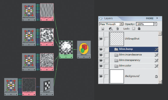
Figure 9.26. (Left) A PSD shading network in the Hypershade window. (Right) The matching PSD file revealed in the Adobe Photoshop Elements Layer window. The scene before the application of Create PSD Network is included on the CD as psd_network_before.ma. The scene after the application of Create PSD Network is included as psd_network_after.ma. The resulting PSD file is included as psd_network_Polyshape.psd.
Bump and displacement mapping can add an extra level of detail to any material. Each has its own unique strengths, weaknesses, and application. Although the Maya Displacement Shader can be difficult to adjust, the Height Field utility provides a rough preview in a workspace view.
Bump maps perturb normals along the interior of a surface at the point of render. They do not, however, affect the outer edges. Nevertheless, the bump effect can easily sell the idea that a surface is rough. When you use a texture as a bump map, middle-gray (0.5, 0.5, 0.5) has no effect. High values cause peaks and low values cause valleys. To set the intensity of a bump map, you can adjust the value of the Bump Depth attribute of the Bump 2D or Bump 3D utility. Bump Depth accepts negative numbers, thus inverting the peaks and valleys.
The simplest way to add a bump map is to click the Bump Mapping checkered Map button in a material's Attribute Editor tab. In this case, a Bump 2D or a Bump 3D utility is automatically connected to the shading network. The Bump 2D utility is designed for standard 2D textures such as File, Checker, or Ramp. The Bump 3D utility is designed for 3D textures such as Brownian, Cloud, or Solid Fractal. If necessary, you can make the bump connections by hand in the Hypershade window. In this case, the outNormal of the bump2d or bump3d node is connected to the normalCamera of the material node. The outAlpha of the texture is connected to the bumpValue of the bump2d or bump3d node. If the outColor of the texture is already connected to another attribute of the material, you can continue to connect the texture's outAlpha to the bumpValue (see Figure 9.27). In this way, only a single place2dTexture node need be adjusted.
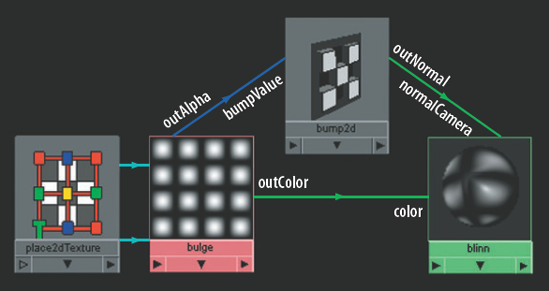
Figure 9.27. A texture is simultaneously connected to a bump2d utility node and a blinn material node.
Bump maps are extremely efficient to render. In fact, bump maps are as convincing as displacement maps in many situations. For example, if a bump map is applied to a surface that sits against a cluttered background, the smooth edges of the surface are difficult to perceive (see Figure 9.28). Motion blur, shadows, and other 3D phenomena also help disguise the bump map's limitations.

Note
The mental ray renderer produces superior results when rendering bump maps and normal maps. For information on mental ray rendering, see Chapter 11. For information on normal mapping, which Is related to bump mapping, see Chapter 13.
Displacement maps distort geometry at the point of render. That is, the assigned surface is tessellated and the resulting vertices are translated a distance based on the source texture. Although displacement maps are more processor intensive, they are more realistic than bump maps. Thus, displacement maps provide the following advantages:
The surface's silhouette is displaced.
Displaced detail casts and receives shadows.
A displacement map can create surface features far more detailed than any other common modeling techniques.
Displacement maps cannot be created through standard material connections in Maya. Instead, you must connect a Displacement Shader to a shading group node. Follow these steps:
Select a material node in the Hypershade window and open its Attribute Editor tab. Click the Go To Output Connection button at the top of the tab (the button is to the left of the Presets button). The tab for the material's shading group node is loaded into the Attribute Editor. Switch to the Shading Group (SG) tab if it's not already selected.
Click the Displacement Mat. checkered Map button in the Shading Group Attributes section. Choose a texture from the Create Render Node window. A displacementShader node is created. The displacement of the displacementShader is connected to the displacementShader of the shading group node (see Figure 9.29). The outAlpha of the texture is connected to the displacement of the displacementShader node. The displacementShader's input and output attribute names are identical.
Render a test frame. To increase the intensity of the displacement effect, increase the value of the texture's Alpha Gain attribute (found in the Color Balance section of the texture's Attribute Editor tab). To reduce the intensity, lower the Alpha Gain.
Alpha Gain is a multiplier that's applied to the texture's Out Alpha attribute. The Alpha Gain default value is 1, which has no effect on the Out Alpha value. An Alpha Gain value of 0 removes the displacement completely. An Alpha Gain value of −1 reverses the displacement. Alpha Offset is an offset factor for the texture's Out Alpha. The Alpha Offset value is added to the Out Alpha value, thus increasing the intensity of the displacement. A negative Alpha Offset reduces the displacement intensity.

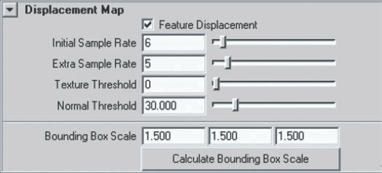
Other aspects of a displacement map can be controlled through the Displacement Map section of the assigned surface's Attribute Editor tab (see Figure 9.30).
The following attributes are particularly useful:
- Feature Displacement
Toggles on or off feature-based displacement. If checked, the Displacement Shader tessellates the assigned surface only in those areas where displaced features occur. If unchecked, the Displacement Shader adds no additional tessellation; in this case, detail contained within the displacement map may be lost if the surface does not have sufficient subdivisions. Maya attempts to make up for the loss of detail inherent with non-feature-based displacement by simultaneously treating the displacement map as a bump map.
- Initial Sample Rate and Extra Sample Rate
Initial Sample Rate determines the size of a sampling grid laid over each polygon triangle. The grid is used to determine whether the triangle should be tessellated. Tessellation is deemed necessary if the contrast between neighboring texture pixels is sufficient. Extra Sample Rate adds additional sampling. In effect, Extra Sample Rate further subdivides the sampling grid applied by Initial Sample Rate. When setting Initial Sample Rate and Extra Sample Rate, use these guidelines:
If the surface is highly subdivided, a low Initial Sample Rate is usually satisfactory.
If the surface is sparsely subdivided and contains large polygon faces, the Initial Sample Rate should be large. Even so, increase the Initial Sample Rate slowly while rendering tests.
Displacement maps with fine detail and/or a great deal of contrast often necessitate high Initial Sample Rate values.
If the displacement requires sharp corners or strongly defined transitions between no displacement and high displacement, you should incrementally raise the Extra Sample Rate value. That said, start with an Extra Sample Rate of 0.
- Texture Threshold
Eliminates unneeded vertices and aims to reduce noise within the displacement. The Texture Threshold value is a percentage of the maximum height variation within the displacement. Any vertex whose difference in height with neighboring vertices is below the Texture Threshold value is removed. The default value of 0 leaves this feature off. When raising the value, do so incrementally. If possible, eliminate any fine noise in the texture map before applying it as a displacement.
- Normal Threshold
Controls the "softness" of the resulting displacement. This attribute's functionality is identical to that of the Set Normal Angle tool (which you can access by switching to the Polygons menu set and choosing Normals > Set Normal Angle). If the angle between two adjacent triangles is less than the Normal Threshold value, the triangles are rendered smoothly. If not, the triangles are rendered with a sharp edge between them.
- Bounding Box Scale
Sets the size of the bounding box used to contain a displacement. If a displacement appears cut off at the peaks or carries other render flaws, gradually increase the X, Y, and Z values. The default values of 1.5, 1.5, 1.5 are adequate for most displacements. Large Bounding Box Scale values increase memory usage. The Calculate Bounding Box Scale button estimates an appropriate bounding box size based on the shading network and world scale of the assigned surface.
Note
Environment textures, which require 3D Placement utilities, are not recommended for use as displacement maps. The resulting calculations will be inaccurate.
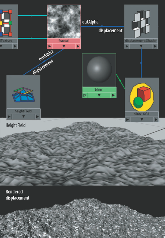
The Height Field utility previews Displacement Shaders in a workspace view. When a texture node is connected to the utility, it creates a plane at 0, 0, 0 and displaces it with the displacement shading network. The Height Field plane cannot be rendered; however, it can be repositioned. The Height Scale attribute of the Height Field utility controls the scale of the previewed displacement. If Height Scale is left at 1, the previewed displacement will match the render of the actual Displacement Shader. The Resolution attribute controls the accuracy of the preview. As an example of the shading network, the outAlpha of a fractal texture node is connected to the displacement of a heightField node (see Figure 9.31). The fractal is also used as the displacement input for a displacement shader node. A Blinn is used as a material. Even though the blinn material node is assigned to a primitive plane with only six spans, a great deal of detail is gained. You can find the Height Field utility in the General Utilities section of the Create Maya Nodes menu.
Every single material, texture, and utility node carries an Extra Attributes section (at the very bottom of the Attribute Editor tab). You can add attributes to this section by choosing Attributes > Add Attributes from the Attribute Editor menu.
In the Add Attribute window, you can set the attribute name with the Long Name field (Maya 2008) or the Attribute Name field (Maya 8.5). Long Name holds the full attribute name as it is used in the Connection Editor and through custom connections (see Figure 9.32). If you check Override Nice Name in Maya 2008, you can set a shorthand name in the Nice Name field. The Nice Name is used in the Channel Box and in the Extra Attributes section of the Attribute Editor tab.
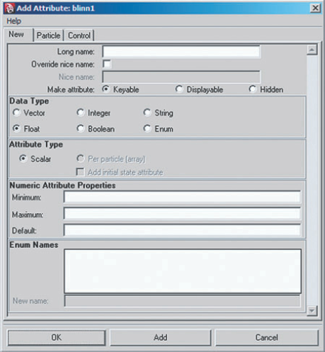
You can set the attribute type with the Data Type attribute. In most cases, Float (number with decimal places) and Integer (whole number) will suffice, although you can choose Vector (three values), String (text), Boolean (on/off), or Enum (drop-down text list).
If you set Data Type to Float or Integer but do not choose values for the Numeric Attribute Properties attributes, a numeric field is created. If you enter values in the Minimum and Maximum fields, a slider is created with that range. The Default field establishes the start position for the slider. The custom attribute appears in the Extra Attributes section of the Attribute Editor tab as well as at the end of the Channel Box channel list. A custom attribute follows the same naming convention as standard attributes:
node_name.attribute_nameAs such, you can use a custom attribute as part of an expression, MEL script, or custom shading network. In the Connection Editor, the custom attribute appears at the end of the list. You can also keyframe custom attributes.
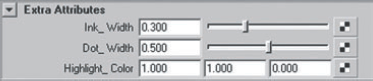
When a custom attribute with a slider is applied to a shading network, a great deal of flexibility is achieved with a minimum amount of effort. For example, sliders are easily connected to the cartoon material detailed in the Chapter 7 tutorial. In this case, three custom attributes are added to the "Cartoon" blinn material node—Ink_Width, Dot_Width, and Highlight_Color (see Figure 9.33). Ink_Width is connected to secondTerm of the ConditionB node. This controls the thickness of the "ink" outline. Dot_Width is connected to the secondTerm of the ConditionA node. This controls the width of simulated halftone. Ink_Width and Dot_Width are float attributes with a minimum value of 0 and a maximum value of 1. Highlight_Color is connected to colorEntryList[4].color of RampA. This changes the color of the "specular" highlight (the highest color on the ramp). Highlight_Color is a vector attribute that provides RGB fields.
In this tutorial, you will prepare the UVs of a polygon model, as shown in Figure 9.34.
Open
piggy_uv.mafrom the Chapter 9 scene folder on the CD. This file contains a polygon model whose UVs are unusable as is.Select the entire surface, switch to the Polygons menu set, and choose Create UVs > Cylindrical Mapping with default options. While the projection manipulator is visible, go to the Channel Box. Change the polyCylProj1 Rotate X value to 270. This orients the projection to the length of the pig. Change Projection Horizontal Sweep to 360. This encloses the surface.
Open the UV Texture Editor. Right-click and choose UV from the marking menu. Click an empty space in the Editor to deselect the UV points. Select the UV points that are stranded far from the main body of points and move them in closer. Select all the UV points and scale them down until they fit within the full UV texture space (represented by the dark-gray box in the upper-right corner of the UV Texture Editor's grid).
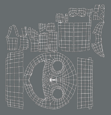
At this step, the pig's snout, ears, and legs have significant overlap. To fix this, you can apply additional mappings. Select all the faces that make up the two ears. You can select the faces in a workspace view or inside the UV Texture Editor. If you right-click and choose Face from the marking menu, you can select faces in the Editor. Choose Create UVs > Planar Mapping with the default settings. Interactively rotate the projection manipulator until it is parallel to the front of the ears. While the manipulator remains visible, return to the UV Texture Editor and move the ear UV points off to the side where they won't overlap other points.
Select all the faces that make up the snout. This should include the snout front, the snout side, and the parts that make up the interior of the smile and nostrils. Choose Create UVs > Automatic Mapping with the default settings. Although the front of the snout appears intact in the UV texture space, other parts are split into little pieces (see Figure 9.35). For now, this is okay. Select and move the resulting UV points off to the side where they won't overlap other points.
Select the faces that make up the front of the snout (the part that looks like a smiley face). Move the faces off to the side where they don't overlap any other parts. Rotate the faces so that they are no longer sideways. Select all the faces that make up the sides of the snout. This might require trial and error. Choose Create UVs > Cylindrical Mapping with the default settings. Move and orient the projection manipulator so that the sides of the snout are fully covered. Move the resulting UV points aside.
Select all the faces that make up the inside of the smile and the nostrils. Choose Create UVs > Planar Mapping with the default settings. Move and orient the projection manipulator so that it faces the front of the snout. Select the resulting UV points and move them aside. While the UV points remain selected, choose Edit UVs > Relax six or seven times. This will allow the inner lip to be flattened out.
Select all the faces that make up the pig's tail. Choose Create UVs > Planar Mapping with the default settings. Move and orient the projection manipulator so that it faces the back of the pig. Select and move the resulting UV points aside.
Select all the faces that make up a single leg. Choose Create UVs > Cylindrical Mapping. With the default settings, move and orient the projection manipulator so that the entire leg is covered. Select and move the resulting UV points aside. Repeat the process for the other legs.
Select the surface in a workspace view. With all the UV points visible in the UV Texture Editor, proceed to move, rotate, and scale the UV shells (groups of UV points) back into the full UV texture space. Use Figure 9.34 as a reference. Once you're satisfied with the UV arrangement, select the surface in a workspace view and choose Edit > Delete By Type > History. This will freeze the UVs.
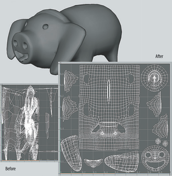
The UV adjustment is complete! This is one of many possible UV preparation approaches and is only a rough pass. You can refine this result in many places. For example, you can reduce the amount of empty space between UV shells. You can fix overlapping UV points on the smile and the bottoms of the legs; re-sew the side of the snout onto the head; and apply additional mappings to separate the front of each ear from its back. Although many fixes require moving points around manually, the technique becomes fairly easy with practice. The final version, as illustrated in Figure 9.34, has been included as piggy_final.ma in the Chapter 9 scene folder on the CD.