
You can use high dynamic range (HDR) images to add realism to any render. The RenderMan For Maya plug-in opens up a whole new world of advanced rendering options. The normal mapping process can record details from a high-resolution surface and impart the information to a low-resolution surface. With the Surface Sampler tool, you can create normal maps, displacement maps, and diffuse maps. The Render Layer Editor gives you incredible control over the batch-rendering process.
Chapter Contents
Understanding the HDRI format
Lighting, texturing, and rendering with HDR images and mental ray
An introduction to RenderMan For Maya
An overview of normal mapping
Managing renders with the Render Layer Editor
Creating the cover illustration
HDRI stands for high dynamic range imaging. An HDR image has the advantage of accurately storing the wide dynamic ranges of light intensities found in nature. In addition, Maya supports HDR images as texture bitmaps and can render HDR images with the mental ray renderer. You can even use HDR images to illuminate a scene without the need for lights.
A low dynamic range (LDR) image carries a fixed number of bits per channel. For example, the majority of Maya image formats store 8 bits per channel. Maya16 IFF, TIFF16, and SGI16 store 16 bits per channel. Thus, an 8-bit image can store a total of 24 bits and 16,777,216 colors. A 16-bit image can store a total of 48 bits and roughly 281 trillion colors. While it may seem 16,777,216 or 281 trillion colors are satisfactory for any potential image, standard 8-bit and 16-bit LDR images are limited by the necessity to store integer (whole number) values. This translates to an inability to differentiate between finite variations in luminous intensity. For example, a digital camera sensor may recognize that an image pixel should be given a red value of 2.3, while a neighboring pixel should be given a red value of 2.1. LDR image formats must round off and store the red values as 2. In contrast, HDR images do not suffer from such a limitation.
Note
Luminous intensity is the light power emitted by a light source or reflected from a material in a particular direction within a defined angle. A bit is the smallest unit of data stored on a computer. Bit depth is simply the description of the number of available bits.
An HDR image stores 32 bits per channel. The bits do not encode integer values, however. Instead, the 32 bits are dedicated to floating point values. A floating point takes a fractional number (known as a mantissa) and multiplies it by a power of 10 (known as an exponent). For example, a floating-point number may be expressed as 7.856e+8, where e+8 is the same as ×108. In other words, 7.856 is multiplied by 108, or 100,000,000, to produce 785,600,000. If the exponent has a negative sign, such as e–8, the decimal travels in the opposite direction and produces 0.00000007856 (e–8 is the same as ×10−8). Because HDR images use floating points, they can store values out of reach to LDR images, such as 2.3, 2.1, or even 2.12647634. Thus, HDR images can appropriately store minute variations in luminous intensity.
Note
You can use Maya's Script Editor as a calculator. For example, typing pow 10 8; in the Script Editor work area and pressing Crtl+Enter produces an answer equivalent to 108. (For descriptions of Maya commands, choose Help > Maya Command Reference from the Script Editor menu.) For common math functions, such as add, subtract, multiply, and divide, you can enter a line similar to float $test; $test = (1.8 * 10) / (5 – 2.5); print $test;.
The architecture of an HDR image makes it perfect for storing a range of exposures within a single file. Hence, the most common use of HDR images is still photography. For example, in Figure 13.1 several exposures of a fluorescent lightbulb are combined into a single HDR image. Any individual exposure, as seen in the top six images in Figure 13.1, cannot capture all the detail of the scene. For instance, in the top-left exposure, the backing a range of exposures within a single file. Hence, the most common use of HDR images is still photography. For example, in Figure 13.1 ground is properly exposed while the lightbulb is little more than a blown-out flare. However, when the exposures are combined into an HDR image, as is demonstrated at the bottom of Figure 13.1, all portions of the scene are clearly visible.
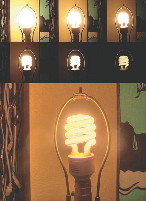
Figure 13.1. (Top) Multiple exposures used to create an HDR image. (Bottom) The resulting HDR image after tone mapping.
The ability to capture multiple exposures within a single file allows for a proper representation of the dynamic range of a subject. When discussing a real-world scene, dynamic range refers to the ratio of minimum to maximum luminous intensity values that are present at a particular location. For example, a brightly lit window in an otherwise dark room may produce a dynamic range of 100,000:1, where the luminous intensity of the light reaching the viewer through the window is 100,000 times greater than the luminous intensity of the light reflected from the dark corner. (On a more technical level, the luminous intensity of any given point in the room or the landscape visible outside the window is measured as n cd/m2, or candela per meter squared; candela is the measure of an electromagnetic field.)
Note
On average, the human eye can perceive a dynamic range of 10,000:1 within a single view and perhaps as much as 1,000,000:1 over an extended period of time.
The main disadvantage of HDR images is the inability to simultaneously view all the captured exposure levels on a computer monitor or television. A process known as tone mapping is required to view various exposure ranges. Tone mapping is discussed in the section "Displaying HDR Images" later in this chapter. A second disadvantage of HDR images is the difficulty with which an HDR image is created through still photography. Special preparation and software is required. Nevertheless, a demonstration is offered in the section "Using Light Probe Images with the Env Ball Texture" later in this chapter.
Maya supports .hdr and OpenEXR image formats. Aside from describing high dynamic range images, the letters HDR describe a specific image format that is based on RGBE Radiance files. To differentiate between HDR as a style of image and HDR as a specific image format, I will refer to the image format by its .hdr extension. The E in RGBE refers to the exponent of the floating point. The Radiance file format was developed by Greg Ward in the late 1980s.
The OpenEXR format was developed by Industrial Light and Magic and was made available to the public in 2002. OpenEXR is extremely flexible and offers both 16-bit and 32-bit floating-point variations. In addition, OpenEXR images can carry an arbitrary number of additional attributes, channels, and render passes (camera color balance information, depth channels, specular passes, motion vectors, and so on). In Maya, OpenEXR is supported by a plug-in. To activate the plug-in, choose Window > Settings/Preferences > Plug-In Manager and activate the Loaded check box for OpenEXRLoader.mll. You may then choose OpenEXR (exr), along with HDR (hdr), from the Image Format attribute drop-down list in the Render Setting window so long as mental ray is the renderer of choice. (The Maya Software renderer is unable to render 32-bit, floating-point formats.)
In addition, mental ray is able to read DDS and floating-point TIFF files. DDS stands for DirectDraw Surface and is an image format developed by Microsoft. DDS files are available in 16-bit and 32-bit variations and are commonly used to store textures for games that employ DirectX. Floating-point TIFFs, on the other hand, supply 32 bits per channel. Floating-point TIFFs are widely used in HDR photography, but are often unwieldy for 3D work due to their large file size. (For example, an average .hdr image may be 3 megabytes, while the equivalent floating-point TIFF takes up 9 megabytes.) To use DDS images, activate the ddsFloatReader.mll plug-in. To use floating-point TIFFs, activate the tiffFloatReader.mll plug-in.
HDR images offer the ability to store huge dynamic ranges. In fact, the RGBE Radiance .hdr format can store luminous values between 10−38 and 1038 cd/m2. Unfortunately, the entire range cannot be viewed on a computer monitor, which has a significantly lower dynamic range capacity. Thus, in order to view the full dynamic range of an HDR image, it must be tone mapped. Tone mapping reduces the extreme contrast present in an HDR image by averaging radiance values; thus, the process is able to convert the HDR image into an 8-bit LDR image without losing properly exposed areas. For example, in Figure 13.2 a HDR image of a sunset is tone mapped, revealing a proper exposure for the sun as well as the surrounding landscape.
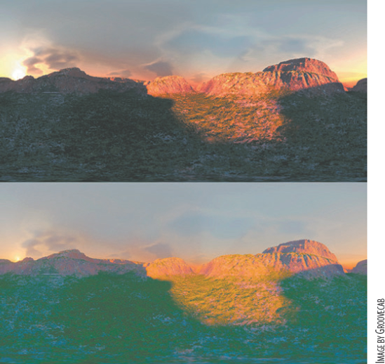
Figure 13.2. (Top) One of many exposures used to create an HDR image. (Bottom) The same HDR image after tone mapping. The sun, sky, canyon, and shadow area are properly exposed.
Several HDR image-processing programs provide tone mapping capabilities, including Photomatix (www.hdrsoft.com) and HDRShop (www.hdrshop.com). Adobe Photoshop also supports a tone mapping option. To view an HDR image in Adobe Photoshop CS3, follow these steps:
Launch Photoshop. Choose File

The image is displayed. However, only a limited portion of the dynamic range is visible (I'll refer to this as the exposure range). To choose a different exposure range, choose View > 32-Bit Preview Options. Adjust the Exposure and Gamma sliders in the 32-Bit Preview Options window. The Exposure slider determines which portion of the exposure range is displayed. The higher the Exposure value, the higher the selected exposure and the brighter the image. The Gamma slider determines the resulting contrast within the displayed image. Both sliders are measured in stops. A stop is the adjustment of a camera aperture that either halves or doubles the amount of light reaching the film or sensor. For the sliders, each stop is twice as intense, or as half as intense, as the stop beside it.
Once the exposure range has been adjusted, you can permanently write out the displayed image as a tone-mapped LDR variation of the original. To do so, choose Image > Mode > 8 Bits/Channel, click OK in the HDR Conversion window, and choose File > Save As.
Note
Technically speaking, HDR images do not store gamma information. In other words, HDR images are not preprocessed with gamma curves in order to make them suitable for a particular display. Instead, HDR images follow the "scene referred standard," which dictates that the format store scene values as close to reality as possible regardless of their ability to be displayed. Eight-bit LDR images, in contrast, follow an "output referred standard," which means that they store colors suitable for an 8-bit display system. (For more information on gamma, see Chapter 6.)
Maya supports the ability to use OpenEXR, .hdr, DDS, and floating-point TIFF images as bitmap textures (assuming that the OpenEXRLoader.mll, ddsFloatReader.mll, and tiffFloatReader.mll plug-ins have been activated). However, when you load an OpenEXR or floating-point TIFF image into a File texture, the texture swatch may appear solid black or white. This is due to Maya's default selection of an exposure range. To adjust the exposure range, follow these steps:
MMB-drag a material into the work area. Map a File texture to its Color attribute. Open the File texture's Attribute Editor tab. Browse for a floating-point TIFF bitmap. A sample floating-point TIFF is included as
tiki.tifin the Chapter 13 images folder.Expand the High Dynamic Range Image Preview Options section (see Figure 13.3). Switch the Float To Fixed Point attribute to Exponential.
Adjust the Exposure slider to reveal different exposure ranges. If Float To Fixed Point is set to Clamp, all the values within the HDR bitmap above 1 are clamped to 1 (hence the image may appear solid white). If Float To Fixed Point is set to Linear, all the bitmap values are normalized (that is, the color curves are rescaled to fit the 0 to 1 range).
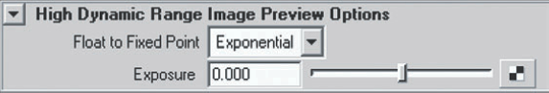
If you load an .hdr or DDS bitmap into a File texture, a median exposure is selected and the Float To Fixed Point attribute has no effect on the texture swatch.
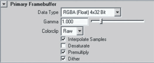
The mental ray renderer is able to render out the full dynamic range of an HDR bitmap used as a texture. This may prove useful when compositing a project that utilizes HDR images. (For example, recent developments in compositing software allow users to interactively "re-light" HDR elements during the composite.) However, additional attributes must be adjusted. Follow these steps:
Assign the material created with the previous set of steps to a primitive plane. Light the plane. Open the Render Settings window and switch Render Using to mental ray. Change the image format to HDR (hdr) or OpenEXR (exr).
Switch to the mental ray tab. Expand the Framebuffer section. In the Primary Framebuffer subsection, change Data Type to RGBA(Float) 4×32 (see Figure 13.4).
Launch a batch render by switching to the Render menu set and choosing Render > Batch Render. A fully dynamic HDR image is rendered to the default project directory. To properly view the image, you must bring it into a program that supports HDR images, such as Photoshop, Photomatix, or HDRShop.
Although a mental ray batch render creates an OpenEXR or .hdr image with the correct dynamic range, the mental ray preview within the Render View window can only provide an LDR version. Nevertheless, it is possible to view different exposure ranges within the Render View window by following these steps:
In the Primary Framebuffer subsection of the mental ray tab of the Render Settings window, change Data Type to RGBA(Byte) 4×8. Render a test frame with the Render View window.
Open the File texture that carries the HDR bitmap and adjust the Color Gain. Lower Color Gain values force the renderer to use lower exposure ranges. Render additional test frames. Different HDR images require different Color Gain values. For example,
tiki.tifrequires a Color Gain value in the range of 0.6, 0.6, 0.6.To change the overall contrast of the rendered HDR bitmap, return to the Primary Framebuffer subsection of the Render Settings window and adjust the Gamma attribute. Higher Gamma values darken the mid-tones of the rendered image. Lower values have the opposite effect.
When you're ready to batch-render once again, return Data Type to RGBA(Float) 4×32, Gamma to 1, and any adjusted Color Gain to its prior value.
In contrast, when an OpenEXR or floating-point TIFF bitmap is rendered with Maya Software through the Render View window or a batch render, Maya uses the exposure range established by the Float To Fixed Point attribute. In other words, only a small portion of the dynamic range is utilized.
The mental ray renderer provides two lens shaders that tone map resulting renders: Mia_exposure_simple and Mia_exposure_photographic. Tone mapping a render is useful when utilizing HDR bitmaps as textures or when surfaces produce super-white values. Applying tone mapping allows you to select a specific exposure range without having to adjust lights or materials. To apply Mia_exposure_simple, follow these steps:
Open the Attribute Editor for the camera used to render a scene. Expand the mental ray section. Click the checkered Map button beside the Lens Shader attribute. Select Mia_exposure_simple from the Create Render Node window (in the Lenses section).
A Mia_exposure_simple node is connected to the camera and is visible in the Hypershade. Adjust the node's attributes and render a test frame.
In terms of attributes, Pedestal offsets the entire color range of the rendered image, either raising it or lowering it. You can give the Pedestal a negative value. The color range is multiplied by the Gain attribute. To lower the exposure range and thus darken the image, lower the Gain below 1. Compression reduces the color range above the Knee value. For example, if Knee is set to 0.5 and Compression is set to 1, then all color values above 0.5 are scaled toward 0.5, thus reducing the highest values in the rendered image. Gamma applies a gamma curve to make the color range nonlinear. A default value of 2.2 matches most PC computer monitors.
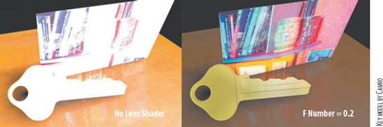
The Mia_exposure_photographic lens shader, on the other hand, is a more advanced tone mapping tool that produces superior renders. It is applied to a camera in the same fashion as Mia_exposure_simple. Many of the attributes, such as Film Iso and Camera Shutter, are designed to match real-world camera setups. Nevertheless, a quick way to lower the exposure level of a rendered image is to enter a low F Number attribute value. For example, in Figure 13.5 a polygon key is assigned to a Blinn with a Diffuse and Specular Roll Off value set to 5. (Any slider can be set to a value higher than its default maximum; see Chapter 6 for more information.) In addition, a second Blinn assigned to a plane has a floating-point TIFF mapped to its Color. As with Mia_exposure_simple, Mia_exposure_photographic tone maps the entire rendered image. (For information on other mental ray lens shaders, see Chapter 12.)
Using the mental ray renderer, you can light a scene with an HDR or LDR bitmap image without the need to create actual lights. You can achieve this with Final Gather or Global Illumination with a technique known as image-based lighting (IBL).
HDR images intended for IBL are created in several styles: angular (light probe), latitude/longitude (spherical), horizontal cubic cross, and vertical cubic cross (see Figure 13.6). The mental ray renderer supports angular and latitude/longitude HDR maps. HDR programs, such as HDRShop, are able to convert images into these special formats (see the section "Using Light Probe Images with the Env Ball Texture" later in this chapter).
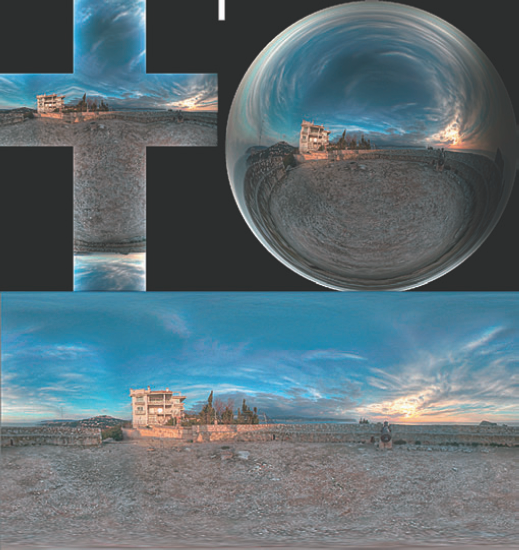
Figure 13.6. (Top left) Vertical cubic cross HDR image. (Top right) Light probe HDR image. (Bottom) Latitude/longitude HDR image.
To illuminate a simple scene with an HDR image, follow these steps:
Open
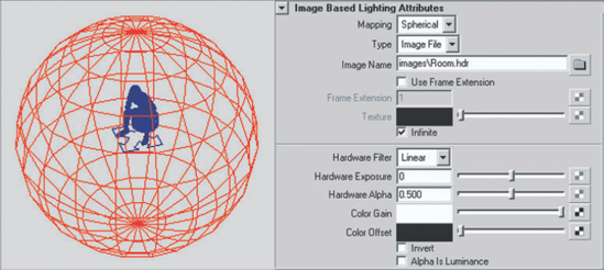
man_hdr.mafrom the Chapter 13 scene folder on the CD. Open the Render Settings window. In the Render Options section of the Common tab, uncheck Enable Default Light. If this is left checked, the default lighting will be added to the Final Gather render. Switch the Render Using attribute to mental ray. In the Environment section of the mental ray tab, click the Image Based Lighting Create button.A mental ray Image Based Lighting (IBL) shape node appears in the Lights tab of the Hypershade window. This generates the orange environment sphere that is placed in the workspace view. Open the environment sphere's Attribute Editor tab (see Figure 13.7).
In the Image Based Lighting Attributes section, click the File button beside the Image Name field and browse for
room.hdrin the Chapter 13 images folder. Set the Mapping attribute to Angular. Angular and light probe maps, although different in name, represent the same type of HDR image.Return to the Render Settings window. Set the Quality Presets attribute to PreviewFinalGather. Render a test frame. Initially, the scene will be dark. (
room.hdrfeatures a darkly lit space.)Return to the IBL shape node's Attribute Editor tab. Click the color swatch beside the Color Gain attribute in the Image Based Lighting Attributes section and enter 5 in the Value attribute field of the Color Chooser window (the color space drop-down menu must be set to HSV). This super-white value will raise the intensity of the HDR image.
Return to the Render Settings window, switch to the mental ray tab, and expand the Final Gathering section. Change Scale to an HSV value of 0, 0, 5. This increases the intensities of the Final Gather point contributions. Render a test. The mannequin appears brighter, but the light colors are very saturated.
One danger of a high IBL shape node Color Gain value is an increased saturation in the color contribution of the HDR image. To counteract this, change Color Offset, also found in the Image Based Lighting Attributes section, to 0.15. Whereas the image color values are multiplied by the Color Gain value, the Color Offset value is added to the image colors. In essence, this adds gray to the image colors, which reduces the saturation. Render out the image. The render is less saturated. A final version of this scene is included on the CD as
man_hdr_final.ma.

Here are a few traits of the IBL shape node renders to keep in mind:
When an image is mapped to an IBL shape node, it appears in the background of the render regardless of the camera's background color or clipping plane settings. However, you can uncheck the Primary Visibility attribute in the Render Stats section of the IBL shape node's Attribute Editor tab. If you do choose to leave the IBL shape node visible, it will not appear in the alpha channel.
In general, renders using HDR images for lighting are not able to produce strong, directional shadows. Nevertheless, you can add standard lights with depth map or raytrace shadows to the scene at any time.
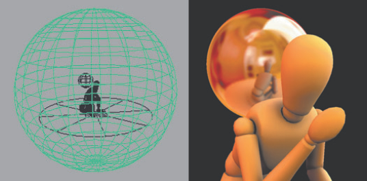
You can add realism by blurring the resulting reflections slightly. For the image in Figure 13.8, the Mi Reflection Blur attribute of the Blinn assigned to the sphere is set to 3 and the Reflection Rays attribute is set to 6.
You can adjust the alignment of the reflection by selecting the IBL environment sphere and rotating it in Y. (Scaling and translating the environment sphere will have no effect on the render if the Infinite attribute is checked in the Image Based Lighting Attributes section.)
If inappropriate dark spots appear in a Final Gather render, adjust the Point Interpolation attribute (found in the Final Gathering section of the mental ray tab of the Render Settings window). Point Interpolation sets the number of Final Gather points that are required when any given pixel is shaded. For the render in Figure 13.8, Point Interpolation was set to 10.
To refine the quality of the Final Gather image, raise the Accuracy value in the Final Gathering section of the mental ray tab of the Render Settings window.
Oddly enough, mental ray's IBL system does not need an HDR image to function. You can map any LDR image to the Image Name attribute of the IBL shape node. The main disadvantage is the difficulty of matching the Spherical or Angular mapping techniques, which are designed for HDR images. Nevertheless, a normal LDR image will illuminate the scene with Final Gather. To avoid the mapping issue, however, you can discard the IBL shape node and its corresponding environment sphere. If an LDR image is mapped to the Ambient Color or Incandescence of a material, mental ray's Final Gather system treats the image as indirect illumination. As such, the material to which the image is mapped need only be assigned to a primitive piece of geometry. For example, in Figure 13.9 a polygon sphere is placed around the mannequin. A blurry LDR JPEG of a room is mapped to the Incandescence of a Blinn, which in turn is assigned to the polygon sphere.
The IBL shape node is actually a collection of three mental ray shaders. The first, an Environment Shader, produces the environment sphere and is used for the basic IBL process. You can use the second, a Photon Emission Shader, to photon trace with caustics and Global Illumination. To do this, you must check the Emit Photons attribute in the Photon Emission section of the IBL shape node's Attribute Editor tab. The Caustics and Global Illumination attributes must also be checked in the Secondary Effects subsection of the Render Settings window. As an example, in Figure 13.10 the mannequin is re-rendered. The mannequin's Blinn material is made semitransparent and given a Refractive Index of 1.4.
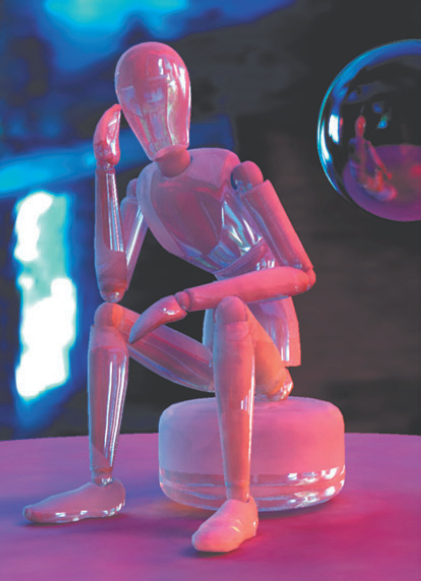
Figure 13.10. A mannequin is lit with an HDR image and rendered with Global Illumination and caustics. This scene is included on the CD as man_hdr_photon.ma.
Adjustments for the Photon Shader are similar to those of a light and include Global Illumination, Caustic Photons, and Exponent attributes. Global Illumination sets the number of photons produced by the environment sphere. Caustic Photons sets the number of caustic photons produced by the environment sphere. Exponent represents the photon energy falloff. An Exponent set to 2 mimics the real world. A low value causes a more gradual energy falloff. In addition, the Standard Emission attribute, when checked, allows the photons created by the Photon Emission Shader to scatter according to the Global Illumination settings in the Render Settings window. The attribute must be checked when rendering caustics. If Standard Emission is unchecked, only the first hit of each photon created by the Photon Emission Shader is stored in the photon map. Last, the Adjust Photon Emission Color Effects attribute, if checked, makes the Color Gain, Color Offset, and Invert attributes available. Color Gain serves as a multiplier for the photon energy. Color Offset serves as an offset for the photon energy. Invert inverts the photon energy. (An intensity of 1 becomes 0 and conversely 0 becomes 1.)
The third shader carried by the IBL shape node is a Light Shader. By checking the Emit Light attribute in the Light Emission section of the IBL shape node's Attribute Editor tab, you can convert the environment sphere into a light source. The Light Shader creates a series of virtual directional lights across the IBL environment sphere and derives their intensities and color from the IBL image file. The virtual lights are perpendicular to the sphere's surface and point toward the origin of world space.
The Quality U and Quality V attributes set the size of a control texture that generates the virtual lights. For each pixel of the control texture, one light is created. To make the render feasible, the Samples attribute places a cap of the number of lights used. The first Samples field determines the minimum number of lights generated. The second Samples field determines the maximum number of additional lights that are randomly added to make the lighting less regular.
Ultimately, the Light Shader creates diffuse lighting and shadows (see Figure 13.11). Since the Light Shader does not require raytracing, Global Illumination, or Final Gather to function, it renders efficiently and quickly. However, if the Quality U and Quality V attributes are raised to high values, the Light Shader render will slow significantly. At the same time, if the Quality U and Quality V values are set too low, the render will appear grainy.

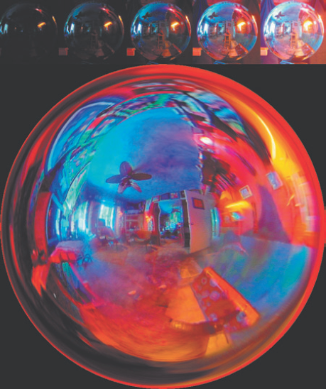
Light probe (angular) HDR images are unique in that they are created by photographing a high-reflective sphere. The sphere offers the advantage of capturing a nearly 360-degree view of an environment. The Env Ball environment texture in Maya, in fact, is designed to support light probe images.
To create a light probe HDR image from scratch, follow these basic steps:
Digitally photograph a reflective sphere in a desired location. The example illustrated in Figure 13.12 employs a 12-inch stainless steel "gazing ball" that is sold as a lawn ornament. Take multiple photos with different F-stops and/or shutter speeds to properly expose all areas of the scene.
Bring the photos into an HDR program that supports the light probe format, such as HDRShop. Combine the photos into a single light probe HDR image. (HDRShop includes detailed instructions in its help files.) It's possible to refine the result by taking photos from multiple angles and stitching the photos together. Taking photos from multiple angles allows you to remove the reflected image of the photographer and camera.
Export the HDR image as an OpenEXR,
.hdr, DDS, or floating-point TIFF bitmap.
To use a light probe image with the Env Ball texture to create a reflection, follow these steps:
Create a test surface and assign it to a Blinn or Phong material. Open the material's Attribute Editor tab. Click the checkered Map button beside Reflected Color. Choose the Env Ball texture from the Create Render Node window (in the Environment Textures section).
Load a light probe HDR image into the Env Ball's Image attribute. If the HDR image is in the OpenEXR or floating-point TIFF format, set the attributes within the High Dynamic Range Image Preview Options section of the file's Attribute Editor tab. If you are using an
.hdror DDS image, a median exposure level is automatically selected by the program.Interactively scale the Env Ball projection icon, found at 0, 0, 0, so that it tightly surrounds the surface. Render a test frame. Raytracing is not required.
If the test surface is spherical, a clear reflection of the light probe image will be visible. However, if the surface is faceted or complex, the reflection may be soft and portions of the image may be severely magnified. To prevent this, adjust the Sky Radius attribute of the envBall node's Attribute Editor tab (in the Projection Geometry section). Sky Radius establishes the world distance from the reflective ball to the real-world sky. In the case of Figure 13.12, there is no sky, so Sky Radius represents the distance to the ceiling.
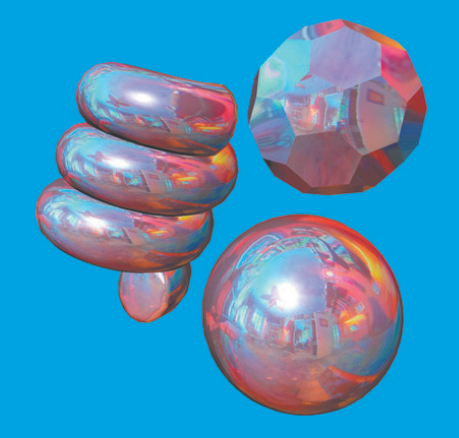
As an additional example, three Env Ball textures are mapped to three Phong materials assigned to three primitives in Figure 13.13. Although the Env Ball assigned to the sphere requires no Sky Radius adjustment, the Env Balls assigned to the helix and soccer ball shape require a Sky Radius value of 1.5. Unfortunately, choosing a Sky Radius value is not intuitive and requires test renders. The Sky Radius units are generic and do not correspond directly to Maya's world units.
RenderMan is a robust renderer developed by Pixar that has been used extensively in feature animation work for over a decade. In recent years, RenderMan has been made available as a plug-in for Maya. (For information on obtaining a copy of the RenderMan For Maya plug-in, visit http://renderman.pixar.com.)
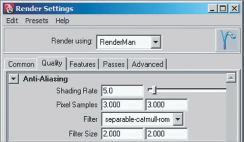
RenderMan For Maya can be activated by checking the RenderMan_for_maya.mll Loaded check box in the Plug-In Manager window. Once the plug-in is activated, RenderMan appears as an option of the Render Using attribute in the Render Settings window. Like other renderers, RenderMan carries its own set of rendering attributes. However, these are spread among four tabs—Quality, Features, Passes, and Advanced (see Figure 13.14).
RenderMan is able to render most of the geometry, materials, and effects in Maya, including depth-of-field, motion blur, raytracing, global illumination, caustics, subsurface scattering, HDR rendering, Maya Fur, Maya Hair, Paint Effects, and particles.
In addition, RenderMan offers a large set of specialty render attributes. You can access the attributes by selecting the object you want to affect and choosing Attributes > RenderMan > Manage Attributes from the Attribute Editor menu. The Add/Remove Attributes window opens (see Figure 13.15).
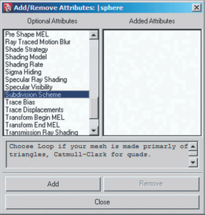
Available rendering attributes are listed in the Optional Attributes field. This is matched to the selected object. For instance, a NURBS surface produces a long list of attributes while a Paint Effects stroke produces a short list. To apply an attribute, highlight the attribute name and click the Add button. The attribute is added to the selected object node and is listed in the Extra RenderMan Attributes section of the node's Attribute Editor tab. Available rendering attributes create a wide array of results on a per-object basis, including:
Raytraced motion blur
Per-surface control of culling and visibility
Per-surface control of diffuse illumination interaction
Subdivision at point of render to negate faceting
Specialized assignment of NURBS curves and other normally unrenderable nodes to shading groups
RenderMan also provides its own advanced variation of a material editor named Slim. You can launch Slim by choosing Window > Rendering Editors > RenderMan > Slim. Much like the Hypershade, Slim allows you to create and edit materials, textures, and custom connections. However, Slim adds many advanced options not available to the Hypershade. In addition, Slim provides its own set of RenderMan materials, textures, and utilities. Any shading network created in Slim can be exported back to Maya. The new shading network appears in the Hypershade and thereafter is accessible to the RenderMan renderer.
The Transfer Maps tool can create normal maps and displacement maps by comparing surfaces. In addition, the tool can bake lighting and texturing information.
Although normal maps are related to bump maps, there are significant differences:
Bump maps store scalar values designed to perturb surface normal vectors on a per-pixel basis. In contrast, normal maps store pre-calculated normal vectors as RGB values; normal maps pay no heed to the surface normal vectors provided by the surface, replacing them instead.
Normal maps are often created by comparing a low-resolution surface to a high-resolution variation of the same surface. Thus, normal maps are able to impart high-resolution detail to a low-resolution surface. Bump maps lack this ability.
Normal maps are not dependent on specific world units and thereby travel more easily between different 3D programs.
To create a normal map with the Transfer Maps window, follow these steps:
Create a new scene. Build a high- and low-resolution version of a single-surface polygon model. (An example file, which includes a simple high- and low-resolution surface, is included as
high_low.maon the CD.)Transform the high- and low-resolution surface to 0, 0, 0 in world space. It's okay if they overlap.
Select the low-resolution surface, switch to the Rendering menu set, and choose Lighting/Shading
Switch the Display drop-down menu, found in the Target Meshes section, to Envelope. Choose Shading
Expand the Source Meshes section of the window. By default, All Other Meshes is listed under the Name attribute. This means that the tool will evaluate all nontarget meshes it encounters within the search envelope. To specify the high-resolution surface as a source surface, select the high-resolution surface and click the Add Selected button. The name of the high-resolution surface appears under the Name attribute.
Click the Normal button (represented by the dimpled ball). Choose a destination for the normal map by clicking the file browse button beside the Normal Map attribute. Choose a File Format. Normal maps can be written in any of the standard Maya image formats. Choose Map Height and Map Width values in the Maya Common Output section. Click the Bake And Close button at the bottom of the window.
At this point, the Transfer Maps tool creates a new material, assigns it to the low-resolution surface, and loads the newly written normal map into a connected bump2d node. The Use As attribute of the bump2d node is set to Tangent Space Normals. To see the result, move the low-resolution surface away from the high-resolution surface and render a test. The result should be similar to Figure 13.16.
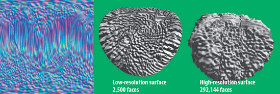
Figure 13.16. (Left to right) Normal map, low-resolution surface with normal map, high-resolution surface. This scene is included on the CD as normal_final.ma. The normal map is included as normal_map.tga in the textures folder.
To improve the quality of the normal mapping process, you can adjust additional attributes:
- Sampling Quality
Found in the Maya Common Output section, Sampling Quality sets the number of samples taken for each pixel of the normal map. This serves as a subpixel sampling system. The higher the values, the more accurate the resulting normal map.
- Transfer In
Found in the Maya Common Output section, Transfer In determines which space the normal map calculations are carried out in. If Transfer In is set to the default World Space, the target and source surfaces can be different sizes. However, they must be positioned at the same world location. If Transfer In is set to Object Space, target and source surfaces can be moved apart; however, the Freeze Transformation tool should be applied while they are positioned at the same world location. If Transfer In is set to UV Space, the surfaces can be dissimilar (different shape or different proportions); however, the surfaces must carry valid UVs for this option to work.
- Map Space
If the Map Space attribute (which is found in the Output Maps section) is set to Tangent Space, the normal vectors are encoded per vertex in tangent space. Tangent space is the local coordinate space of a vertex that is described by a tangent vector, a binormal vector, and the surface normal. The tangent vector is aligned with the surface's U direction. The binormal vector is aligned with the surface's V direction. If Map Space is set to Object Space, the resulting normal map takes on a rainbow hue. This is due to the surface normals always pointing in the same direction in object space regardless of the translation or rotation of the surface in world space. The Object Space option is only suitable for surfaces that are not animated.
You can also create normal maps through the Render Layer Editor; an example is included in the section "Using Presets" later in this chapter.
The best normal map cannot improve the quality of a low-resolution surface's edges. However, the Transfer Maps tool is able to preserve the edge details of the high-resolution surface by creating a displacement map for the low-resolution surface. Steps to create a displacement map are almost identical to the steps to create a normal map:
Move the high-resolution surface and the low-resolution surface to the same point in world space. Assign the low-resolution surface to a new material. With the low-resolution surface selected, choose Lighting/Shading > Transfer Maps. The low-resolution surface is listed in the Target Meshes section. Select the high-resolution surface and click the Add Selected button in the Source Meshes section.
Click the Displace button. Click the file browse button beside the Displacement Map field and choose a destination for the displacement map to be written out. Choose an appropriate File Format and Map Width and Map Height.
Switch the Connect Maps To attribute, found in the Connect Output Maps section, to Assigned Shader. Click the Bake And Close button at the bottom of the window.
Move the low-resolution surface away from the high-resolution surface. Render a test frame. In this case, the displacement map is automatically connected to a displacementShader node, which in turn is connected to the Displacement Shader attribute of the material's shading group node.
Unfortunately, displacement maps created with the Transfer Maps tool often produce a "quilting" effect along the original polygon edges. That is, the faces of the low-resolution surface appear to be "puffed out" among the high-resolution surface detail. To reduce this potential problem, follow these guidelines:
Change the Maximum Value attribute (found in the Output Maps section). Raising the value reduces the amount of contrast in the displacement map. In turn, this reduces the intensity of any quilting artifacts and prevents plateaus from forming when parts of the map become pure white. The ideal value varies with the surfaces involved.
Increase the Filter Size attribute (found in the Maya Common Output section) to add blur to the map.
Incrementally raise the Initial Sample Rate and Extra Sample Rate attributes of the target surface. (These attributes are found in the Displacement Map section of the surface's Attribute Editor tab.) This will increase the accuracy of the displacement.
Adjust the Alpha Gain and Alpha Offset attributes of the File node that carries the displacement map. (See Chapter 9 for more information.)
Touch up the map in Photoshop. The Displacement Shader interprets a 0 value as no displacement and a 1 value as maximum displacement.
As an example, in Figure 13.17 a displacement map is generated by the Transfer Maps tool using a high-resolution and low-resolution plane. The high-resolution plane, on the left, has 18,342 polygon triangles. The low-resolution plane, on the right, has 72 triangles. In the Transfer Maps window, the Map Resolution is set to 512×512, the Maximum Value to 5, and the Sampling Quality to Medium (4×4). The Alpha Gain of the resulting displacement map's file node is raised to 10. The Initial Sample Rate and Extra Sample Rate of the low-resolution surface are set to 20 and 10, respectively.

You can "bake" lighting, texture, and shadow information with the Transfer Maps tool. In this situation, a textured source creates a color bitmap for a target surface. The Transfer Maps tool provides two attributes to choose from for this operation: Diffuse Color Map and Lit And Shaded Color Map. Diffuse Color Map simply captures a source surface's color without regard to lighting or shadows. Lit And Shaded Color Map captures all the source surface's information, including specular highlights, bump maps, ambient color textures, and so on (see Figure 13.18). You can map the resulting color bitmap to the low-resolution surface to reduce render times (by avoiding bump mapping, shadow casting, and the like). The use of Diffuse Color Map and Lit And Shaded Color Map attributes is identical to the creation of a displacement map or normal map. The Diffuse Color Map is activated with the Diffuse button, and the Lit And Shaded Color Map is activated with the Shaded button.

Render management is an inescapable part of animation production. Complex projects can easily generate hundreds, if not thousands, of rendered images. The complexity is magnified when objects are rendered in separate passes or when shading components are addressed individually. Fortunately, Maya's Render Layer Editor makes the task more efficient.
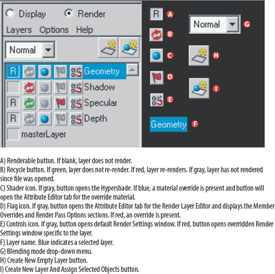
The Layer Editor is accessible by clicking the Show The Channel Box And Layer Editor icon on the status bar. The Layer Editor is composed of two sections, which you can toggle between by clicking the Display or Render radio button. The Display section of the Layer Editor is known as the Display Layer Editor. The Render section is known as the Render Layer Editor (see Figure 13.19). You can access the Render Layer Editor directly by choosing Window > Rendering Editors > Render Layer Editor.
By default, Maya places all objects on a master layer. The master layer is not visible in the Render Layer Editor until a new layer is created. To create a new layer and assign objects to that layer, you can choose one of these two approaches:
Choose objects in the scene and click the Create New Layer And Assign Selected Objects button.
Click the Create New Empty Layer button. While the master layer is highlighted in the layer list, select objects in the scene. Click the new layer in the layer list. The objects will be invisible but will remain selected. Right-click the new layer's name and choose Add Selected Objects from the shortcut menu.
You can add additional objects to a preexisting layer at any time by right-clicking a layer name and choosing Add Selected Objects. Conversely, you can remove objects by choosing Remove Selected Objects. To rename a layer, double-click the layer name and enter a new name in the Name field of the Edit Layer window. To change the order of the layers, MMB-click and drag any layer name up or down the layer stack.
You can edit the layer membership of any object by opening the Relationship Editor and switching to the Render Layers view (see Figure 13.20). You can access this view directly by choosing Window > Relationship Editors > Render Layers. You can add objects to a layer by clicking the layer name in the left column and clicking the object name in the right column. Once an object is included, its name appears in the left column under the layer name. To remove an object from a layer, click the object name in the right column.

When a new layer is created, it is rendered by default. To toggle off the render status, click off the R symbol beside the layer's name in the Render Layer Editor.
Maya provides six special effect methods for combining layers. These techniques are accessible through the Blend Mode drop-down menu (see Figure 13.19). The modes correspond to layer blend modes in Photoshop and include Normal, Lighten, Darken, Multiply, Screen, and Overlay. For example, if three layers are activated with the R symbol and each layer has a different blend mode, the final rendered image will contain a blended version of the three layers (see Figure 13.21). This assumes that the Render View window is set to composite. (In the Render View window, choose Render > Render All Layers >
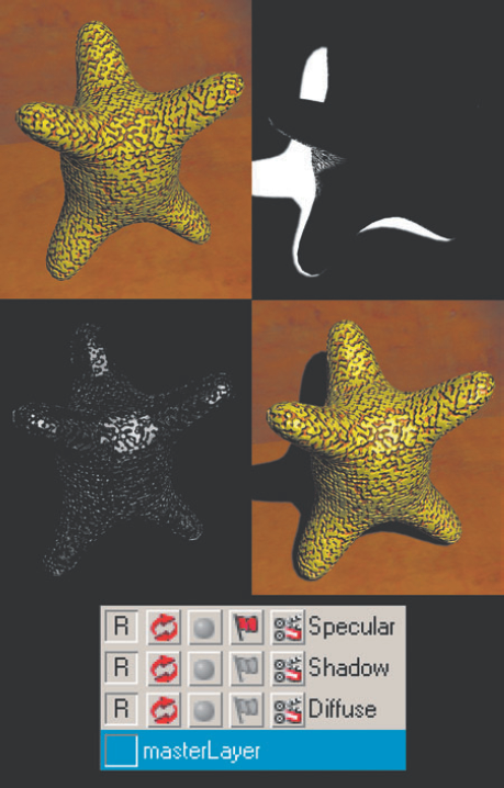
Figure 13.21. (Upper left) Diffuse layer render. (Upper right) Shadow layer render. (Middle left) Specular layer render. (Middle right) Blended layers result. (Bottom) Render Layer Editor. Diffuse layer Blending Mode is set to Normal. Shadow layer Blending mode is set to Multiply. Specular layer Blending Mode is set to Screen. This scene is included on the CD as layer_blending.ma.
Note
You can force Maya to save each layer of the Render Layer Editor as a separate layer in a Photoshop file. To do so, switch the Image Format in the Render Settings window to PSD Layered. In the Render View window, choose Render > Render All Layers >
Each render layer that you create receives a long list of Member Overrides. The overrides allow a particular layer to overturn specific attributes of the objects rendered in the layer (these attributes are also known as render flags). The master layer, by comparison, receives no overrides.
To access the Member Overrides section in the Render Layer Editor's attribute tab, click the flag icon beside the layer name (see Figure 13.19 earlier in this chapter).
For example, in the Member Overrides section, you can switch the Casts Shadows attribute from Use Scene to Override On and thus force all objects assigned to the layer to not cast shadows. When an override is activated, the flag icon in the Render Layer Editor turns red. Additional override attributes control motion blur, visibility, and double-siding.
The Render Layer Editor's attribute tab also contains a Render Pass Options section (see Figure 13.22). Checking or unchecking the Render Pass Options attributes isolates specific shading components. If Beauty is checked, all standard shading components are rendered. However, if only Color is checked, the color component renders by itself. Diffuse produces the diffuse component. Shadow isolates shadows in the alpha channel. Specular isolates the specular highlights. (The Render Pass Options technique will not create an appropriate alpha channel for the Specular attribute.) Splitting an animation into such shading components is a common technique in the animation industry; the resulting renders allow for a maximum amount of flexibility during the compositing process. For an example of this technique, see the section "Step-by-Step: Creating the Cover Illustration" at the end of this chapter.

You can override the settings of the Render Settings window per layer by clicking the small "controls" icon directly to the left of the layer name (see Figure 13.19 earlier in this chapter). (The icon features a tiny picture of a motion picture clapboard.)
When the controls icon is clicked, the Render Setting window opens in an override mode. The Render Setting window indicates this by including the layer name in the window title bar (for example, Render Settings (layer2)). You can change any of the Render Settings window attributes. However, to make the changes a recognized override for the layer, follow these steps:
Right-click over an attribute name and choose Create Layer Override from the shortcut menu. The attribute name turns orange, indicating that it carries an override for the active layer (see Figure 13.23).
Change the value or option for the overridden attribute.
To remove an override, right-click the attribute name and choose Remove Layer Override from the shortcut menu. The attribute automatically takes its value or option from the default Render Setting window.
You can launch the Render Settings window with its layer-centric overrides at any time by clicking the controls icon of a specific layer. You can change all the attributes and options within the Render Settings window per layer, including the renderer used. For example, if a scene features a glass on a table, you can render the glass layer with mental ray and raytracing while rendering the table layer with Maya Software and no raytracing.
The master layer receives its render settings from default Common and render-specific tabs of the Render Settings window. However, once a new layer is created, the default Render Settings window displays tabs for all available renderers. Any attribute that is not overridden for a layer takes its setting from the default Common and render-specific tabs.
The Render Layer Editor provides a series of presets that allow a given layer to be temporarily assigned to a new material and shading group node. All the surfaces assigned to the layer are affected by the assignment. The assignment only occurs on the layer the preset is applied to and does not influence the assignment of materials on other layers.
To apply a preset, right-click a layer name and choose Presets > preset name from the shortcut menu. Descriptions of the presets follow:
- Luminance Depth
Creates a Z-buffer style render in the RGB channel of the image. This is achieved by assigning the surfaces to a Surface Shader material. The material's Out Color is connected to a custom shading network, which derives the distance to camera from a Sampler Info node. You can use Luminance Depth images to create artificial depth-of-field and other "depth priority" effects in a compositing program.
- Geometry Matte
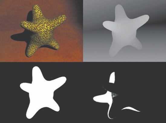
Generates a solid matte effect in the RGB channels by assigning the surfaces to a Surface Shader material with a 100 percent white Out Color. In the example shown in Figure 13.24, the star shape is assigned to the layer but the backdrop geometry is not. Solid mattes are useful for compositing operations and filters.
- Specular and Diffuse
Isolate their namesake shading components by remotely controlling attributes in the Render Pass Options section. (See "Creating Member Overrides and Render Pass Options" earlier in this chapter.)
- Occlusion
Ambient occlusion refers to the blocking of indirect or diffuse light. Creases, cracks, and crevices on real-world objects are often darker due to indirect and diffuse light being absorbed or reflected by nearby surfaces. In 3D, however, this does not occur automatically. Thus, ambient occlusion renders are useful for darkening renders where they are normally too bright or washed out.
The Occlusion preset achieves ambient occlusion by assigning surfaces to a Surface Shader material with a Mib_amb_occlusion mental ray shader mapped to the Out Color. Unfortunately, it is difficult to blend the Occlusion preset render with the master layer in the Render Layer Editor. Much more control is gained if the Occlusion preset render is combined with a beauty or diffuse render in a compositing program (see Figure 13.25).
- Normal Map
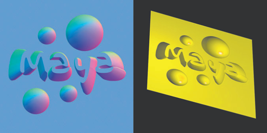
Renders a tangent-space normal map. You can use the image for compositing operations that require surface normal direction information. You can also map the render to the Bump Value of a Bump 2D utility; the result is similar to a bas-relief (see Figure 13.26). If the Use As attribute of the Bump 2D utility is set to Tangent Space Normals and the mental ray renderer is utilized, the result is fairly clean.
You can create your own custom presets by right-clicking the layer name and choosing Create New Material Override > material. You have the option to choose any material from the Maya and mental ray library. The new material appears in the Hypershade window, where it can be renamed and edited. The material override will not be active until it is assigned to a layer, however. Once assigned, every surface in the layer is assigned to the override material. To assign the override material, right-click the layer name and choose Assign Existing Material Override > override material name. You can access the Attribute Editor tab of a previously assigned material override by clicking the shader icon beside the layer name (see Figure 13.19 earlier in the chapter). You can remove an override by right-clicking the layer name and choosing Remove Material Override.
The cover illustration was created specifically for this book. Since the amount of time available to create the render was limited, I combined standard lighting and texturing techniques with various shortcuts.
The model of the woman, known as Masha, was built by Andrey Kravchenko and is commercially available via www.turbosquid.com. Masha's polygon count, including clothing, is approximately 45,000 triangles. For purposes of the illustration, however, modeling adjustments were made to the face. In addition, the torso was split into two overlapping surfaces—one for her skin and one for the semitransparent lace shirt. Masha was given a no-frills character rig and posed into place. Other models, such as the spotlights and mannequin, were either culled from the first edition of the book or commercially purchased (see Figure 13.27).
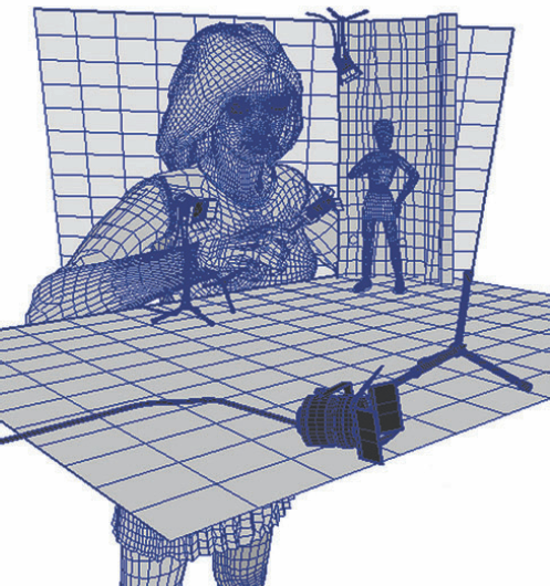
As for lighting, standard spot, directional, and ambient lights were employed (see Figure 13.28). Two spot lights illuminated the mannequin and represented the throw the prop spotlights. An additional spot light served as a key. A directional light created a rim and represented light arriving from the blue-green background. Two ambient lights shared the duty as fill light.

The rendering was managed with the Render Layer Editor. This allowed various parts of the scene, such as side curtain, the individual prop spotlights, the mannequin, and various parts of Masha herself, to be rendered out in separate passes. It also allowed for any given layer to have different material overrides and presets applied to further separate shading components. For example, the mannequin was rendered with beauty, diffuse, specular, ambient occlusion, and shadow passes (see Figure 13.29). This diversity of render passes allowed for a great deal of flexibility in the compositing phase, whereby each render was given different sets of filters, color adjustments, opacities, and blending modes.
Each render pass received a different renderer and secondary rendering effect based on its contents and desired result. While some passes used Global Illumination or Final Gather with mental ray, others relied on Maya Software. Global Illumination proved to be the most effective with the mannequin and curtain, while Final Gather proved invaluable for creating warmness for Masha's face. The spotlight props, on the other hand, proved satisfactory with Maya Software.
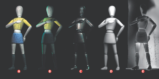
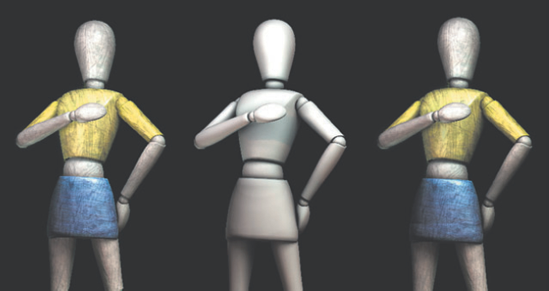
Figure 13.29. Render passes for mannequin shown side by side. A) Diffuse. B) Beauty with alternative lighting. C) Specular. D) Ambient occlusion. E) Shadow (with curtain).
Another advantage of splitting a render into multiple passes is the ability to re-light for each pass. That is, because each render pass was created separately, there was no need to keep the lighting static throughout the rendering process. For instance, lighting that made Masha's face look appealing was not successful for her hand. Therefore, when it came time to create the render pass for the hand, the lights were repositioned. Although the Render Layer Editor cannot keep tabs on the positions of lights, it is fairly easy to save different versions of the scene file. The trick, in this case, is to be explicit with the scene file naming. For instance, any given scene file would follow the naming convention part_component_version.mb (for instance, hand_diffuse_v2.mb).
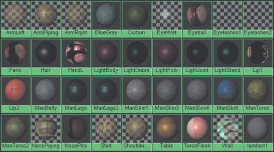
The Masha model was accompanied by a set of custom bitmaps. However, these were discarded in favor of new textures. In addition, the UVs of the face were remapped to support more detail. All other surfaces in the scene were assigned to custom materials with custom bitmap textures. In the end, 35 materials were created (see Figure 13.30).
While the majority of material shading networks remained mundane with standard Color, Bump Mapping, and Specular Color connections to File textures, the skin texture utilized a custom shading network (see Figure 13.31). Three different variations of the face bitmap texture were mapped to the Color, Ambient Color, Specular Color, and Bump Mapping. The face bitmaps were further adjusted by blending the File textures with other File, Mountain, or Leather textures through Layered Texture nodes. The Diffuse attribute was controlled by Sampler Info, Remap Value, and Multiply utilities, allowing a custom diffuse falloff to be created; this created the illusion of translucency. Time limitations prevented the use of more accurate subsurface scattering techniques.

To create the reflections on the stands of the spotlight props, an Env Sphere texture was mapped to the Reflected Color of an assigned Blinn. A rough draft render of the scene was loaded into the Image attribute of the Env Sphere, providing the basic colors established by the scene.
To create the transparency necessary for the lace shirt, a high-resolution, grayscale bitmap was created and mapped to the shirt material's Transparency (see Figure 13.32). The detail in the map was so fine, however, that rendering high-quality shadows of the lace on Masha's torso proved excessively time-consuming. As a result, the shirt surface had its Casts Shadows attribute checked off and the lace shadows were created in the composite.
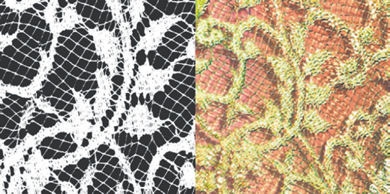
Figure 13.32. (Left) Detail of lace Transparency bitmap. (Right) Detail of lace in final illustration.
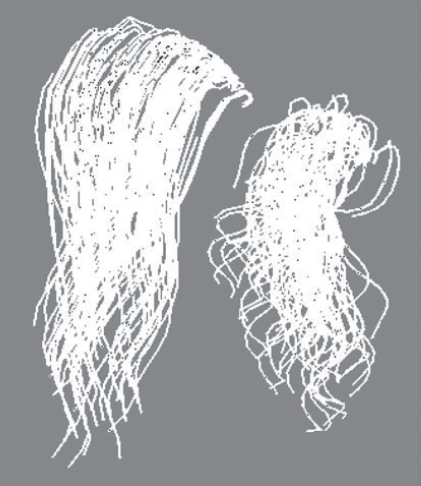
Another area that proved difficult was Masha's hair. The original model came with a surface that represented the hair's volume, but had little detail. In order to get a sense of individual hairs, the surface was removed and replaced by Paint Effects system. The Paint Effects were not left in their default state, however, but were converted to polygons. This allowed small sections of the hair mass to be dynamically simulated on a stand-in object, converted with the Modify > Convert > Paint Effects To Polygons tool, and then arranged within the scene. Once several basic hair "clumps" were created, in fact, they could be duplicated and overlapped to create greater complexity. Each clump was created with the hairWetCurl Paint Effects brush with custom attribute settings to give it an appropriate amount of randomness, segments, and curvature (see Figure 13.33). Each clump had approximately 25,000 polygons once converted. The final hair mass contained over 500,000 polygons. The clumps were assigned to a Hair Tube Shader material, which provided a unique variation of anisotropic specularity.
The final resolution of each render pass was 2130×2130. Render times varied from 10 minutes to 1 hour depending on the complexity of the render layer and the choice of renderers and secondary rendering effects. Images were saved as Targas with an alpha channel. All Targas were brought into Adobe After Effects, where they were adjusted, filtered, combined, and rendered as a final image. The final image was imported into Adobe Photoshop for touch-ups. The total time invested in the illustration was approximately 35 hours. A detail of the illustration is shown in Figure 13.34.
There are many ways to approach any given render in Maya. Although this book has demonstrated various methods, they are by no means the only approaches available. Flexibility and resourcefulness are equally valuable assets when creating 3D. I sincerely hope that Advanced Maya Texturing and Lighting, Second Edition inspires you to develop brand-new techniques.
