Simply put, a material determines the look of a surface. Although it's easy enough to assign a material and a texture to a surface and produce a render, many powerful attributes and options are available to you. At the same time, a rich historical legacy has determined why materials and textures work the way they do. You can map a wide range of 2D textures to materials, creating an almost infinite array of results. Simple combinations of textures and materials can lead to believable reproductions of real-world objects.
Chapter Contents
Theoretical underpinnings of shading models
Review of Maya materials
Review of 2D textures
Descriptions of extra texture attributes
Material and texture layering tricks
Using common mapping techniques to reproduce real materials
A shader is a program used to determine the final surface quality of a 3D object. A shader uses a shading model, which is a mathematical algorithm that simulates the interaction of light with a surface. In common terms, surfaces are described as rough, smooth, shiny, or dull.
In the Maya Hypershade and Multilister windows, a shading model is referred to as a material and is represented by a cylindrical or spherical icon. Ultimately, you can use the words shader and material interchangeably.
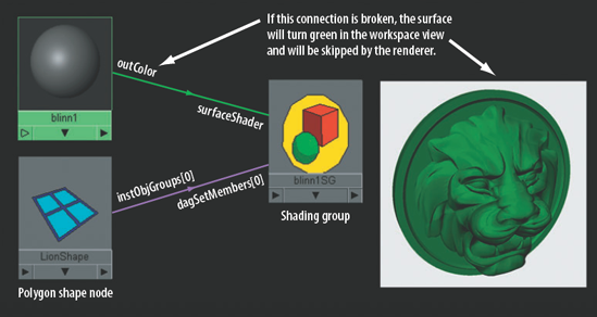
A shading group, on the other hand, is connected to the material as soon as it's assigned. The shading group's sole function is to associate sets of surfaces with a material so that the renderer knows which surface is assigned to which material. The shading group does not provide any definition of surface quality. If the connection between a shading group node and material is deleted, the assigned surface appears solid green in the workspace view and is skipped by the renderer (see Figure 4.1). When a material is MMB-dragged into the Hypershade work area, it is automatically connected to a new shading group. If you select a material through the Create Render Node window, however, you have the option to uncheck the With Shading Group attribute; in this case, no new shading group is created.
The Lambert material carries common attributes: Color, Transparency, Ambient Color, Incandescence, Bump Mapping, Diffuse, Translucence, Translucence Depth, and Translucence Focus. In Maya, the Lambert node is considered a "parent" node. That is, Phong, Phong E, Blinn, and Anisotropic materials inherit their common attributes from the Lambert material. In each case, the attributes function in an identical manner. (For a more detailed discussion of nodes and the Transparency attribute, see Chapter 6. For information on the Bump Mapping attribute, see Chapter 9.) Maya's Lambert material uses a diffuse-reflection model in which the intensity of any given surface point is based on the angle between the surface normal and light vector. In order for Maya's Lambert material to smoothly render across polygon faces, it borrows from other shading models, such as interpolated or Gouraud shading. With Gouraud, the intensity of any given point on a polygon face is linearly interpolated from the intensities of the polygon's vertex normals and two edge points intersected by a scan line.
Note
The Smooth Shade All option (Shading > Smooth Shade All through a workspace view menu) is able to interpolate across polygon faces to produce a smooth result. In contrast, the Flat Shade All option (Shading > Flat Shade All through a workspace view menu) applies a single illumination calculation per polygon face, which leads to faceting.
NURBS surfaces, while based on Bezier splines, are converted to polygon faces at the point of render by the renderer. Hence, all the shading model techniques in this chapter apply equally to NURBS surfaces. If Flat Shade All is checked through a workspace view menu, a NURBS primitive sphere appears nearly identical to its polygon counterpart.
Calculations involving diffuse reflections utilize Lambert's Cosine Law. The law states that the observed radiant intensity of a surface is directly proportional to the cosine of the angle between the viewer's line of sight and the surface normal. As a result, the radiant intensity of the surface, which is perceived as surface brightness, does not change with the viewing angle. Hence, a Lambertian surface is perfectly matte and does not generate highlights or specular hot spots. Physically, a real-world Lambertian surface has myriad surface imperfections that scatter reflected light in a random pattern. Paper and cardboard are examples of Lambertian surfaces. The law was developed by Johann Heinrich Lambert (1728–77), who also served as the inspiration for the Lambert material's name.
The term diffuse refers to that which is widely spread and not concentrated. Hence, the Diffuse attribute of the Lambert material represents the degree to which light rays are reflected in all directions. A high Diffuse value produces a bright surface. A low Diffuse value causes light rays to be absorbed and thereby makes the surface dark.
The Ambient Color attribute represents diffuse reflections arriving from all other surfaces in a scene. To simplify the rendering process, the diffuse reflections are assumed to be arriving from all points in the scene with equal intensities. In practical terms, Ambient Color is the color of a surface when it receives no light. A high Ambient Color value will cause the object to wash out and appear flat.
The Incandescence attribute, on the other hand, creates the illusion that the assigned surface is emitting light. The color of the Incandescence attribute is added to the Color attribute, thus making the material appear brighter.
Note
You can use the Ambient Color and Incandescence attributes as irradiant light sources when rendering with Final Gather. For more information, see Chapter 12.
The Translucence attribute simulates the diffuse penetration of light into a solid surface. In the real world, you can see this effect when holding a flashlight to the back of your hand. Translucence naturally occurs with hair, fur, wax, paper, leaves, and human flesh. Advanced renderers, such as mental ray, are able to simulate translucence through subsurface scattering (see Chapter 12 for an example). Maya's Translucence attribute, however, is a simplified system. The higher the attribute value, the more the scene's light penetrates the surface (see Figure 4.2).

Figure 4.2. Different combinations of Translucence, Translucence Depth, and Translucence Focus attributes on a primitive lit from behind. This scene is included on the CD as translucence.ma.
A Translucence value of 1 allows 100 percent of the light to pass through the surface. A value of 0 turns the translucent effect off. Translucence Depth sets the virtual distance into the object to which the light is able to penetrate. The attribute is measured in world units and may be raised above 5. Translucence Focus controls the scattering of light through the surface. A value of 0 makes the scatter of light random and diffuse. High values focus the light into a point.
The Phong shading model uses diffuse and ambient components but also generates a specular highlight based on an arbitrary shininess. In general, specularity is the consistent reflection of light in one direction that creates a "hot spot" on a surface. With the Phong model, the position and intensity of a specular highlight is determined by reading the angle between the reflection vector and the view vector (see Figure 4.3). A vector, in this situation, is a line segment that runs between two points in 3D Cartesian space that represents direction. (For a deeper discussion of vectors and vector math, see Chapter 8.)
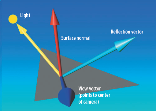
If the angle between the light vector and the surface normal is 60 degrees, the angle between the reflection vector and the surface normal is also 60 degrees. In this way, the reflection vector is a mirrored version of the light vector. If the angle between the reflection vector and view vector is large, the intensity of the specular highlight is either low or zero. If the angle between the reflection vector and view vector is small, the intensity of the specular highlight is high. The speed with which the specular highlight transitions from high intensity to no intensity is controlled by the Cosine Power attribute. The higher the Cosine Power value, the more rapid the falloff, and the smaller and "tighter" the highlight.
Both Gouraud and Phong shading models produce specular highlights. However, Phong produces a higher degree of accuracy, particularly with low-resolution geometry. As with the Gouraud technique, Phong reads vertex normals. Phong goes one step further, however, by interpolating new surface normals across the scan line. The angle between a surface normal at the point to be rendered (c) and the light vector determines the intensity of that point (see Figure 4.4).

Ultimately, 3D specular highlights are an artificial construct. Real-world specular highlights are reflections of intense light sources (see Figure 4.5).

Figure 4.5. (Top left) A classic specular highlight appears on an eye. (Top right) A closer look at the eye reveals that the specular highlight is the reflection of the photographer's light umbrella. (Bottom left) A glass float with a large specular highlight. (Bottom middle) With the exposure adjusted, the float's specular highlight is revealed to be the reflection of a window. (Bottom right) The window that creates the reflection.
The Blinn shading model borrows the specular shading component from the Phong model but treats the specular calculations in a more mathematically efficient way. Instead of determining the angle between the reflection vector and view vector, Blinn determines the angle between the view vector and a vector halfway between the light vector and view vector. This frees the specular calculation from specific surface curvature. In practical terms, you can make the Maya Phong and Blinn materials produce nearly identical highlights (see Figure 4.6). Maya's Blinn material uses the Eccentricity attribute to control specular size and the Specular Roll Off attribute to control specular intensity.
When it comes to the position of the specular highlight, both Phong and Blinn re-create Fresnel reflections, whereby the amount of light reflected from a surface depends on the angle of view (which is the opposite of diffuse reflections). That is, when the view changes, the highlight appears at a different point on the surface (see Figure 4.7).
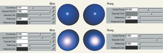
Figure 4.6. Small and large specular highlights on Blinn and Phong materials. This scene is included on the CD as blinn_phong.ma.
Note
Although Maya's Blinn and Phong materials are able to change the location of the specular highlight as the view changes, they are unable to accurately change the inherent intensity of the specular highlight. The Studio Clear Coat utility plug-in, however, solves this limitation. For a demonstration, see Chapter 7.
Maya's Phong E material is a variation of the Phong shading model. Phong E's specular quality is similar to both Phong and Blinn. The Roughness attribute controls the transition of the highlight core to the highlight edge. A low Roughness value will cause the highlight to fade off quickly, whereas a high Roughness value causes the highlight to have a diffuse taper in the style of a Blinn material. The Highlight Size attribute controls the total size of the highlight. The Whiteness attribute allows an additional color to be blended into the highlight between the colors established by the Color and Specular Color attributes. The Specular Color attribute is the color of the highlight at its greatest intensity.
Blinn, Phong, and Phong E highlights will become distorted as they approach the edge of a surface with a high degree of curvature. In addition, Blinn, Phong, and Phong E produce elongated highlights on cylindrical objects (see Figure 4.8).

Figure 4.8. Blinn, Phong, and Phong E materials assigned to primitive spheres, cylinders, and planes. This scene is included on the CD as blinn_phong_cylinders.ma.
When comparing the material's highlights to photographs of real-world equivalents, it's apparent that the Blinn, Phong, and Phong E models are fairly realistic (see Figure 4.9). Phong and Phong E materials do have a slight advantage on the edge of a spherical surface, where specular reflections naturally grow in width.
Note
Fresnel reflections are named after Augustin-Jean Fresnel (1788–1827), who drafted theories on light propagation. The Gouraud shading model was presented by Henri Gouraud in 1971. The Phong shading model was created by Bui Tuong Phong in 1975. The Blinn shading model was developed in 1977 by James Blinn, who was also a pioneer of bump and environment mapping.

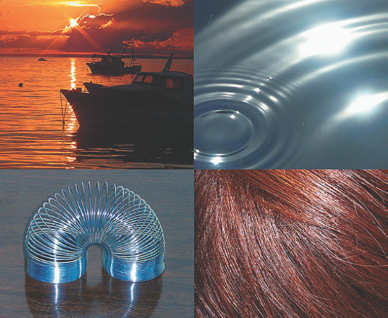
The anisotropic shading model produces stretched reflections and specular highlights. The model simulates surfaces that have microscopic grooves, channels, scratches, grains, or fibers running parallel to one another. In such a situation, specular highlights tend to be elongated and run perpendicular to the direction of the grooves. The effect occurs on choppy or rippled water, brushed, coiled, or threaded metal, velvet and like cloth, feathers, and human hair (see Figure 4.10).
The anisotropic shading model is opposite that of isotropic shading models used by such materials as Blinn or Phong. With isotropic models, the quality of the specular highlight does not change if the assigned surface is moved or rotated. With anisotropic models, a change in the surface's translation or rotation can significantly alter the resulting highlight. As a simple demonstration, two NURBS spheres are assigned to default Blinn and Anisotropic materials and are translated and rotated (see Figure 4.11).
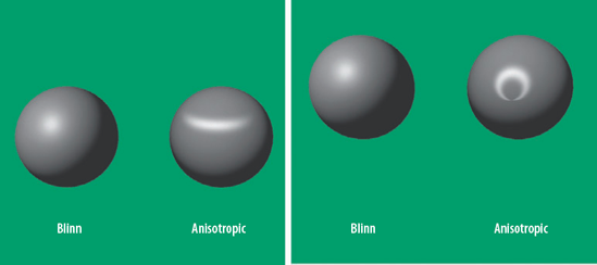
Figure 4.11. The specular highlight of an Anisotropic material changes with translation and rotation of the assigned sphere on the right. This scene is included on the CD as anisotropic_spin.ma. A QuickTime movie is included as anisotropic_spin.mov.
CDs and DVDs produce strong anisotropic highlights due to their method of manufacture. You can re-create these in Maya with the following steps:
Create a new scene. Choose Create > NURBS Primitives > Circle with the default settings. Select the resulting circle and choose Edit > Duplicate.
Select the duplicated circle and reduce the scale so that it is the appropriate size for the CD's center hole. Select both circles, switch to the Surfaces menu set, and choose Surfaces > Loft.
Select the new surface and assign it to a new Anisotropic material. Open the material's Attribute Editor tab. Set Spread X to 100, Spread Y to 1, Roughness to 0.8, and Fresnel Index to 9.5.
Create a point light and place it above the surface. Render a test. At this point, the specular highlight is white. To insert colors into the highlight, click the checkered Map button beside Specular Color. From the Create Render Node window, choose Ramp. Open the new ramp texture in the Attribute Editor tab. Set the Interpolation to Smooth. Render a test. The highlight now emulates the color shift of real CDs (see Figure 4.13). If the colors run in a direction opposite that of a real CD, switch the top and bottom handles of the ramp texture.
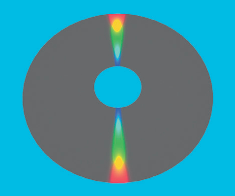
Figure 4.12. The anisotropic highlight of a CD is re-created in Maya. This scene is included on the CD as anisotropic_cd.ma.
The Anisotropic attributes work in the following way:
- Angle
Determines the angle of the specular highlight.
- Spread X
Sets the width of the grooves in x direction. The x direction is the U direction rotated counterclockwise by the Angle attribute.
- Spread Y
Sets the width of the grooves in y direction, which is perpendicular to the x direction. If Spread X and Spread Y are equal, the specular highlight is fairly circular.
- Roughness
Controls the roughness of the surface. The higher the value, the larger and the more diffuse the highlights appear.
- Fresnel Index
Sets the intensity of the specular highlight.
- Anisotropic Reflectivity
If checked, bases reflectivity on the Roughness attribute. If unchecked, the standard Reflectivity attribute determines reflectivity.
For information on raytracing and an additional example of an Anisotropic material used to create the specular highlights on glass, see Chapter 11.
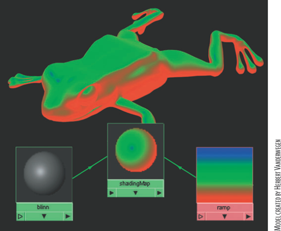
Maya's Shading Map material remaps the output of another material. In other words, the Shading Map discreetly replaces the colors of a material, even after the qualities of that material have been calculated. In a basic example, the Out Color attribute of a Blinn material is mapped to the Color of a Shading Map material (see Figure 4.13). The Out Color of a Ramp texture is mapped to the Shading Map Color of the Shading Map material. In turn, the Shading Map material is assigned to a polygon frog. Where the Blinn material normally shades the model with a dark color, the bottom of the Ramp is sampled. Where the Blinn normally shades the model with a light color, such as a specular highlight point, the top of the Ramp is sampled.
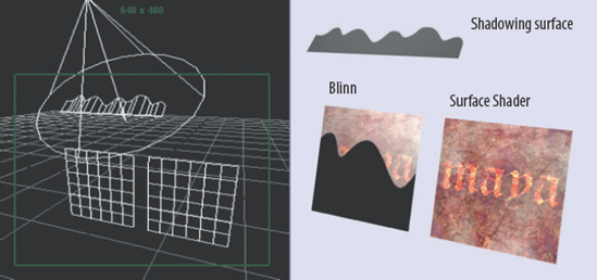
Maya's Surface Shader material is a "pass through" node. That is, the material was designed to make arbitrarily named inputs recognizable to the renderer. The material does not contain shading properties and will not take into account any light or shadow information. A surface assigned directly to a Surface Shader material appears self-illuminated. Any texture mapped to the Out Color attribute of the Surface Shader comes through the render with all its original vibrancy intact (see Figure 4.14). This makes the Surface Shader ideal for background skies and brightly lit signs. The material is also well suited for custom cartoon materials in which shadowing and highlights are provided by a custom network and not by actual lights. For a cartoon material example, see Chapter 7.
Maya's Use Background material allows the assigned surface to pick up color from a camera's Background Color attribute or image plane. For example, in Figure 4.15 a photo of a quiet town is loaded into the default persp camera as an image plane (choose View > Image Plane > Import Image from the camera's workspace view menu). A NURBS plane is aligned to the perspective of the photo's street. The plane is assigned to a Use Background material. The resulting render places the shadow of a polygon craft on top of the street.
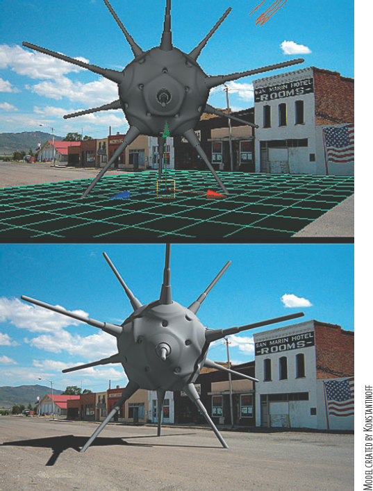
Figure 4.15. The Use Background material is assigned to a primitive plane, thus placing a shadow on a photo of a street. A simplified version of this scene is included on the CD as use_background.ma. The image is also included in the textures folder as street.tif.
If the image plane is removed from the camera and the polygon craft is assigned to a 100 percent transparent Lambert material, the shadow is rendered by itself and appears in the alpha channel (see Figure 4.16). This offers an excellent means to render shadows out on their own pass. If shadows are rendered separately, you can composite them back onto a static background. For an example of this technique, see Chapter 10. For more information on alpha channels, see Chapter 6.

Figure 4.16. The Use Background material isolates a shadow in the alpha channel. A simplified version of this scene is included on the CD as background_shadow.ma.
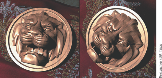
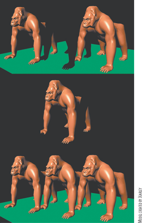
The Use Background material also serves as an "alpha punch" that cuts holes into other objects. For this to work, the camera's Background Color attribute (found in the Environment section of the camera's Attribute Editor tab) should be set to black. For example, in Figure 4.17 three polygon gorillas stand close together, partially occluding each other. In a first render pass (see the top of Figure 4.17), a Use Background material is assigned to the center gorilla while the other surfaces are assigned to several Blinn materials. As a result, the center gorilla cuts a hole into the other two. As a second render pass (see the middle of Figure 4.17), the Use Background material is assigned to the two outer gorillas and the ground plane. The center gorilla is assigned to a Blinn. As a result, the two outer gorillas cut a hole into the center gorilla. When the two render passes are brought into a compositing program, they fit together perfectly (see the bottom of Figure 4.17). This works whether the objects are static or are in motion. When used in this fashion, the Use Background material allows characters and objects in a scene to be rendered separately without any worry of which object is in the front and which is in the back.
Note
You can isolate shadows with Maya's Render Layer Editor. For a detailed description of the editor, see Chapter 13.
Note
Three materials—Hair Tube Shader, Ocean Shader, and Ramp Shader—are not discussed in this chapter. The Hair Tube Shader is designed for the Maya Hair System, which is covered briefly in Chapter 3. The Ocean Shader is designed specifically for fluid dynamic ocean simulations and has no other general purpose. The Ramp Shader is reviewed in Chapter 7.
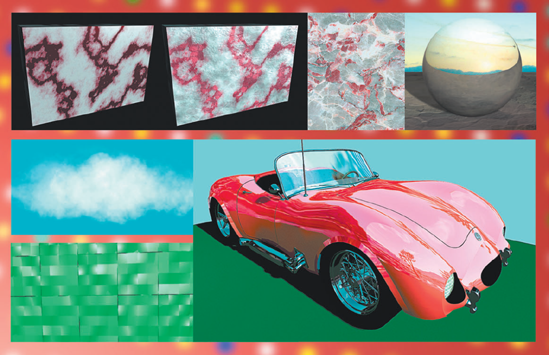
Maya 2D textures can be grouped into the following categories: cloth, water, Perlin noise, ramp, bitmap, and square. Aside from bitmaps, all these textures are generated procedurally. That is, Maya creates these textures with specialized algorithms that create repeating patterns.
The Cloth texture is unique in that it generates interlaced fibers. Aside from obvious use in clothing, it can be adjusted to generate various organic patterns such as reptile scales. For example, in Figure 4.18 a Cloth texture is mapped to the Bump Mapping attribute of a Blinn material.
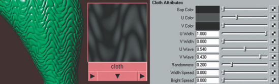
Figure 4.18. The Cloth texture is adjusted to create scales. This material is included on the CD as cloth_scales.ma.
The regularity, or irregularity, of the cloth pattern is controlled by ten attributes. Gap Color, U Color, and V Color set the color of the virtual threads. U Width and V Width determine the width of the threads in the U and V direction. U Wave and V Wave insert wave-like distortion into the cloth pattern. Randomness harshly distorts the pattern in the U and V directions. Width Spread randomly changes the thread widths. Bright Spread randomly darkens of lightens the thread colors.
By default, the Water texture produces overlapping wave patterns. Although the default is not particularly suited for realistic liquid, you can adjust the attributes to create other patterns found in nature. For example, in Figure 4.19 a Water texture is applied to a plane as a bump map and is adjusted to emulate wind-blown sand.

Figure 4.19. (Left) Wind-blown sand forms patterns on a dune. (Right) A 3D facsimile utilizing the Water texture. This scene is included on the CD as water_sand.ma.
Critical attributes of the Water texture include:
- Number Of Waves
Sets the number of waves used to create the pattern.
- Wave Time and Wave Velocity
Wave Time controls the placement of the waves. Gradually increasing the value will cause the waves to "roll" across the texture as if part of a body of water. Wave Velocity sets the speed by which the waves move if Wave Time is changed. Both attributes are designed for keyframe animation.
- Wave Amplitude
Controls the height of the waves. Higher values introduce greater degree of contrast into the pattern.
- Wave Frequency and Sub Wave Frequency
Wave Frequency sets the fundamental frequency of the waves. Higher values create waves that are narrower and more tightly packed. Sub Wave Frequency overlays a higher frequency onto the base waves, which makes the wave pattern more irregular.
- Smoothness
Smoothness blurs the wave pattern. A higher value makes the pattern softer and less detailed. (The generated pattern is never hard-edged, even when Smoothness is turned down to 0.)
The Concentric Ripple Attributes section sets aside another ten attributes for creating and controlling circular ripples. You can isolate the concentric ripples by setting Number Of Waves to 0.
In addition, you can use the Water texture to distort flags and other cloth-like surfaces. For example, in Figure 4.20 a Water texture is mapped to the Bump Mapping attribute of a Blinn material. The Repeat UV attribute of the Water's 2D Placement utility is kept below 1 in the U and V direction.
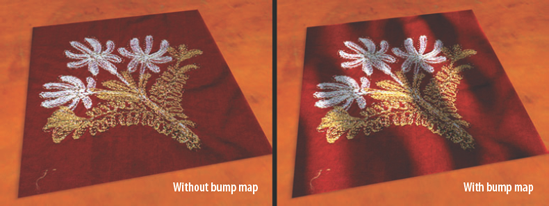
Figure 4.20. A Water texture is applied to a plane as a bump map, giving the cloth texture extra dimension. This scene is included on the CD as water_cloth.ma.
Note
The Ocean texture is designed for Maya's Ocean System. The Fluid Texture 2D texture uses Maya's fluid dynamic simulation. For more information, refer to the "Fluid Effects" Maya help file.
Perlin noise was invented by Ken Perlin in the early 1980s as a means of generating random patterns from random numbers. You can use Perlin-based 2D textures to break up surface regularity. For example, you can map the Maya Noise texture to a material's Specular Color to make a specular highlight appear more irregular (see Figure 4.21).

Figure 4.21. (Left) A Blinn assigned to a polygon frog shows little variation in the specular highlight. (Right) A Noise texture mapped to the Specular Color of the same Blinn produces a more complex result. A simplified version of this scene is included on the CD as specular_noise.ma.
In addition, you can map a Noise texture to a File texture's Color Gain to dirty up an otherwise clean bitmap. For an example, see "Stacking Materials and Textures" later in this chapter.
Maya's Fractal texture is a more complex variation of classic 2D Perlin noise in which turbulence (the averaging of multiple scales) is added for detail. The majority of attributes are identical to the Noise texture. The attribute list for both the Noise and Fractal texture is quite long but will be detailed in Chapter 5.
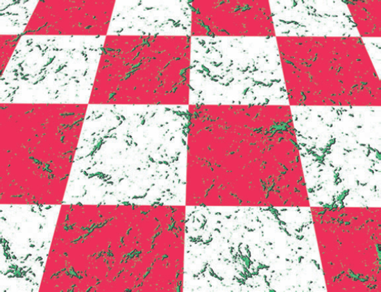
Maya's Mountain texture, on the other hand, is a variation of Perlin noise that lacks a smoothing function. It simulates a simplified mountain range where snow occurs at a particular elevation (as viewed from above). Although it's not possible to create a realistic mountain with the Mountain texture, you can use the texture to create granular patterns. For example, in Figure 4.22 two Mountain textures are respectively mapped to the Color and Bump Mapping attributes of a Phong material, creating the illusion of green debris and scum on a floor. A Checker texture is mapped to the Snow Color of the Mountain connected to the Phong's Color attribute, thus providing the red and white tiles.
The Mountain texture's unique attributes follow:
- Amplitude, Snow Color, and Rock Color
Amplitude sets the amount of Rock Color that appears "through" the Snow Color. A low value favors Snow Color in the coloring scheme. As demonstrated in Figure 4.22, Snow Color can be mapped with another texture. The same is true for Rock Color.
- Boundary
Controls the raggedness of the Snow Color to Rock Color transition. A low value creates smoother transitions and favors the Snow Color. A high value creates numerous interlocking nooks and crannies.
- Snow Altitude, Snow Dropoff, and Snow Slope
Snow Altitude determines the "altitude" at which Snow Color appears. Higher values increase the overall amount of snow. Snow Dropoff controls the rapidity at which the snow disappears at lower altitudes. The lower the Snow Dropoff value, the less snow there is. Snow Slope is the angle at which snow sticks to the virtual mountain. The higher the Snow Slope value, the more snow there is.
The Ramp texture allows selected colors to transition in the U or V direction. The texture carries a total of nine ramp Type attribute options and seven Interpolation attribute options, supporting a wide range of results (see Figure 4.23).
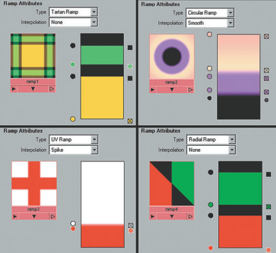
Figure 4.23. Unusual combinations of ramp types and interpolations. These textures are included on the CD as ramps.ma.
Note
Ramp textures are often employed in custom shading networks. For a demonstration of a Ramp used to create a custom wireframe render, see Section 4.1 of the Additional_Techniques.pdf on the CD. For a demonstration of a Ramp used to create a window reflection in an eye, see Section 4.2 of the same file. Ramp textures are also used to create an iron shading network later in this chapter, a custom cartoon material in Chapter 7, and per-particle colors in Chapter 8.
Importing custom bitmaps, whether as File, PSD File, or Movie textures, is the most powerful way to achieve realism and detail in Maya. File textures are used extensively in the custom shading networks demonstrated in Chapters 5 through 7. Movie textures are simply variations of File textures. Movie textures will read any movie format supported by Maya, including Windows Media Player AVI files on Windows systems and QuickTime on Macintosh systems. In order to use all the frames contained within the movie, you must check the Use Image Sequence attribute. Both File and Movie textures are able to accept numbered image sequences. Once again, Use Image Sequence must be checked for all the frames to be read.
Square textures are generated by repeating color blocks or lines in the U and V directions. Square textures include Bulge, Grid, and Checker. The Bulge texture can be thought of as a blurry Grid texture. Both Bulge and Grid are often useful for bump mapping. If either the U Width or V Width attribute of the Grid texture is set to 0, parallel grooves are generated in one direction. The Checker texture is handy for checking UV distortions on surfaces (see Chapter 9).
Several texture attributes are often overlooked, but are nonetheless quite useful. These include Filter, Filter Offset, Filter Type, Invert, and Color Remap.
By default, many Maya textures are filtered, whether they are procedural or bitmap. This is necessary to prevent aliasing problems. In general, aliasing artifacts occur when the detail contained within a texture is smaller than corresponding screen pixels. The problems are most noticeable when textures have a high degree of contrast and the camera or surface is in motion. In this situation, a moiré pattern is often formed (see Figure 4.24 for an extreme example). Although many of the anti-aliasing attributes in the Render Settings window reduce such problems (see Chapter 10), texture filtering remains a necessity of the 3D process.
In Maya, the filtering process is controlled by the Filter and Filter Offset attributes, found in the Effects section of the texture's Attribute Editor tab. Filter forces the renderer to employ a lesser or greater degree of filtering. In essence, filtering averages the texture pixels, thus blurring the texture. The lower the Filter value, the lesser the degree of filtering and the sharper the texture. The higher the Filter value, the greater the degree of filtering and the blurrier the texture. You can stylistically add or subtract detail from a texture by adjusting the Filter attribute. For example, in Figure 4.25 the effect of a large Filter value is a blurry Grid texture. Whereas Filter controls the degree of filtering in camera space, Filter Offset controls the amount of blur in texture space. In practical terms, the Filter Offset value is added to the Filter value for an extra degree of blurring.
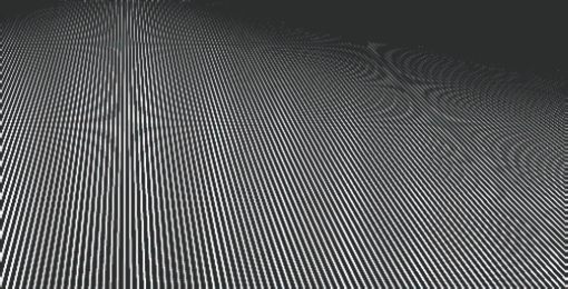
Figure 4.24. Moiré patterns formed by texture details that are smaller than corresponding screen pixels
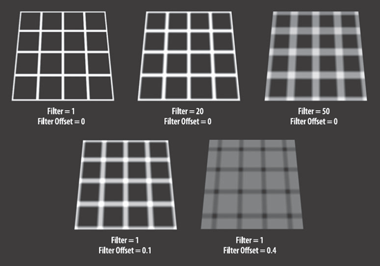
Figure 4.25. A Grid texture with six different Filter and Filter Offset settings. This scene is included on the CD as grid_filter.ma.
Note
Cloth, Bulge, Ramp, Water, Fluid Texture 2D, Fluid Texture 3D, Granite, Leather, and Snow textures do not possess filtering attributes.
File, Movie, and PSD File textures offer additional controls for the filtering process. You can set the Filter Type attribute, found at the top of the textures' Attribute Editor tab, to Off, Mipmap, Quadratic, Quartic, Gaussian, and Box.
Off turns off the filtering process and removes the Filter and Filter Offset attributes. Although this will speed up the render, moiré and stair-stepping artifacts will most likely appear.
Mipmap applies the mipmapping process. In this case, Maya stores averaged color values for multiple sizes of each texture. The sizes linearly decrease (for example, 512 × 512, 256 × 256, 128 × 128, and so on). When the renderer tackles an individual screen pixel, it determines the most appropriately sized mipmap. If the pixel falls over a distant surface, it recalls a small size. If the pixel falls over a surface in the immediate foreground, it recalls a large size. The angle between the surface and the camera is part of the equation. An oblique surface (one that is not perpendicular to the line of sight) induces a smaller mipmap, and a non-oblique surface induces a larger one. To increase the accuracy of the mipmap selection, Maya often averages a consecutive pair of mipmaps (for example, 512 × 512 and 256 × 256).
Gaussian shares its name with filters common to digital paint programs, such as Adobe Photoshop. Gaussian filters blur an image by convolving an array representing the original image and a second, smaller array known as a kernel. In simple terms, convolution allows the arrays to be multiplied together by "sliding" the kernel across the image array. The kernel itself contains a bell-shaped distribution of values that causes a predictable effect on different frequencies within the image. Higher frequencies equate to small details. Low frequencies equate to large image features. The end effect of a Gaussian filter is a blur that softens fine details without destroying large image features or negating edges.
Quadratic and Quartic are approximations of the Gaussian filter type that employ different bell-shaped distributions in their kernels. Both filters are optimized for speed. Quadratic offers the best balance of efficiency and quality, and is therefore the default option for Filter Type.
Box is the simplest filtering option available. Box gives equal weight to all sampled image pixels; hence, it does not preserve edges as well as other filter types. As a comparison, a TIFF image of a street is loaded into a File texture (see Figure 4.26). The File texture is mapped to the Out Color attribute of a Surface Shader material, which is assigned to a plane. The plane is rendered with Off, Mipmap, Quadratic, and Box Filter Type options. Off produces the most contrast; unfortunately, the sharp edges are likely to cause stair-stepping artifacts when the camera or plane is animated. Mipmap produces a softer result while allowing the building's "Meat Market" sign to be fairly readable. Quadratic is very close to Mipmap, but offers a slight increase in edge contrast. In this example, Quadratic erodes away the center horizontal line of the sign's first "E." Box creates the blurriest result, which make the sign difficult to read. In addition, Box creates harsh kinks in vertical lines. In particular, the left vertical edge of the sign has a severe stair-step artifact.
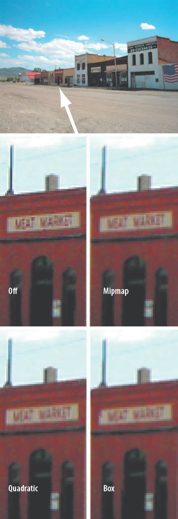
Figure 4.26. Detail of a 1024 × 768 bitmap, loaded into a File texture and rendered with four Filter Type options. This scene is included on the CD as filter_comparison.ma.
Two extra attributes are available to File, Movie, and PSD File textures: Pre Filter and Pre Filter Radius. Pre Filter, if checked, applies additional image-space filtering to the loaded map. The filtering occurs before any other operation is applied to the map. The higher the Pre Filter Radius value, the blurrier the image.
Note
If a texture's Filter Type is set to Box, Quadratic, Quartic, or Gaussian and the texture's Filter is set to an excessively high value, the texture will become pixilated and blocky. To intentionally create a heavy blur on a texture, leave Filter at its default value and raise Filter Offset by small increments (such as 0.1). Although Pre Filter will blur the texture, its blur cannot reach the strength supplied by the Filter Offset.
The Invert check box, found in the Effects section of a texture's Attribute Editor tab, inverts the colors of the texture. The result is identical to the Reverse utility (see Chapter 8). If a color is pure white (RGB: 1, 1, 1), the inverted result is black (RGB: 0, 0, 0). If a color is yellow (RGB: 1, 1, 0), the inverted result is blue (RGB: 0, 0, 1). You can predict the results by picking an opposite side of the Maya color wheel.
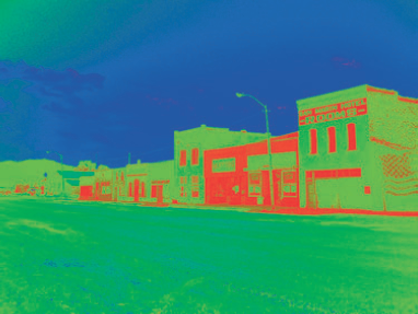
The Color Remap Insert button, also found in the Effects section, attaches an Rgb To Hsv utility and a Ramp texture to the shading network. The new network color-shifts the original texture (see Figure 4.27). The portion of the texture that has low color values is given colors from the bottom of the Ramp. The portion of the texture that has high color values is given colors from the top of the Ramp. If you change the Ramp colors, the colors of the texture automatically change. (See Chapter 6 for a demonstration of the Rgb To Hsv utility in a custom network.)
The Layered Shader material offers an easy method by which to combine two or more materials. For example, in Figure 4.28 a Blinn and a Lambert material are mapped to a Layered Shader material. The Blinn's Color is set to red with a hot specular highlight. The Lambert's Color is set to yellow and carries no specularity. The Blinn and Lambert are represented by the purple box icons in the icon field of the Layered Shader Attributes section of the Layered Shader's Attribute Editor tab. The Blinn and Lambert each receive a Transparency attribute. Which set of attributes is visible depends on which box icon is highlighted. You can switch between the box icons at any time by clicking them. If you hold your mouse over an icon, the name of the connected material is revealed. Although only two materials are connected to the Layered Shader in this example, you can connect three, four, five, or more. You can disconnect materials by clicking the small × below the corresponding icon. How the materials are mixed depends on each material's Transparency value. In the case of Figure 4.28, the Blinn, represented by the left icon, has a Transparency value set to 50 percent gray. The Lambert, represented by the right icon, has a Transparency value set to 0 percent black. The resulting Layered Shader contains a 50 percent mix of each material, producing an orange color. The specular highlight becomes more intense since the colors are added.
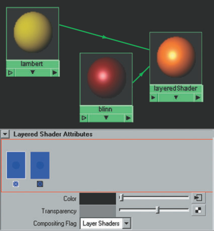
Figure 4.28. Two materials are blended with the Layered Shader material. This material is included on the CD as layered_shader.ma.
To choose the correct value for the various Transparency sliders in the Layered Shader material, follow these guidelines:
The horizontal row of purple box icons is similar to a vertical stack of layers in Adobe Photoshop. The leftmost icon is equivalent to the highest layer in Photoshop, and the rightmost box is equivalent to the lowest layer.
If the Transparency value of the first material (the one that is represented by the leftmost icon) is set to 0 percent black, the first material obscures all other materials.
The last material mapped to the Layered Shader (represented by the rightmost icon) does not need its Transparency adjusted above 0 percent black. If the Transparency value is raised above 0 percent black, the resulting material becomes semitransparent.
The Layered Shader material works equally well with textures. As such, the material provides the Compositing Flag attribute to determine how to output the blended items. If you are blending materials, set Compositing Flag to Layer Shaders. If you are blending textures, set Compositing Flag to Layer Texture.
Note
You can map materials and textures to the Layered Shader material by MMB-dragging material and texture icons into the Layered Shader Attributes icon field of the Layered Shader's Attribute Editor tab. A purple box icon appears for each material or texture added.
The Layered Texture texture is almost identical to the Layered Shader material. However, it prefers connections from textures and will not function with materials. Any mapped texture receives a purple box icon. In the place of Transparency sliders, Layered Texture includes Alpha sliders. In addition, each texture connected to the Layered Texture receives a Blend Mode attribute. The Blend Mode attribute determines how each texture will combine with the texture just below it. In terms of icons, the Blend Mode attribute controls how each icon will be combined with the icon to its immediate right. A number of Blend Mode options (Add, Subtract, Multiply, Difference, Lighten, Darken, Saturate, Desaturate, and Illuminate) are identical to the equivalent layer blend modes in Adobe Photoshop and other digital-imaging programs. The None option makes the texture 100 percent opaque, preventing any lower texture (or right-hand icon) from appearing. If an Alpha attribute is mapped with a black and white texture, the In option cuts out the lower texture in the shape of the Alpha map; black areas become holes in the lower texture. With the same alpha map, the Out option inverts the cut. The Over option places the texture with the Alpha map on top of the lower texture as if it were a decal; black areas become holes for the upper map.
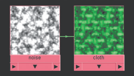
Although the Layered Texture texture offers a great deal of control when blending separate textures, you can simply map the Color Gain attribute of a texture (found in the Color Balance section of a texture's Attribute Editor tab). Color Gain works as a scaling factor—the texture's Out Color attribute is multiplied by the Color Gain color or map. For example, in Figure 4.29 a Noise texture is mapped to the Color Gain of Cloth texture, thus dirtying it. Conversely, the Color Offset attribute works as an offset factor. Whereas Color Gain functions as a multiplier, Color Offset simply adds its value to Out Color. Thus, a black Color Offset will have no effect on the texture. A 50 percent gray Color Offset will brighten the texture by adding RGB values of 0.5, 0.5, 0.5 to the texture's Out Color.
You can adjust a Blinn material to emulate a wide range of surfaces. In this section, steps for achieving wood, metal, and plastic using common map attributes are detailed. To simplify the demonstration, a single bitmap texture, rusty.tif, is used in each case (see Figure 4.30). (For details on creating glass, water, and ice, see Chapter 11.)
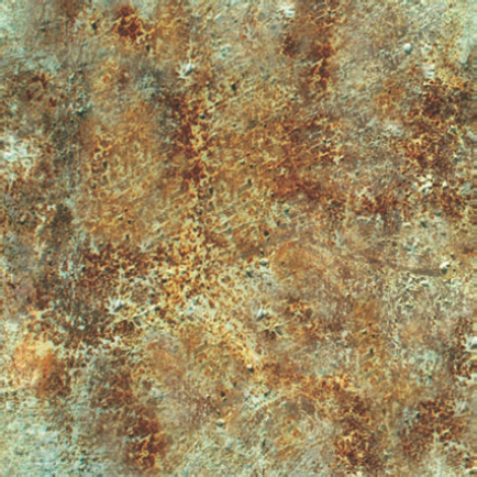
Figure 4.30. A noisy, dirty, rusty bitmap texture that can be applied in numerous ways. This bitmap is included on the CD as rusty.tif.
Before I discuss specific texturing examples, a quick look at placement utilities and naming conventions is necessary. The 2D Placement utility is connected automatically to a shading network when a material's checkered Map button is clicked and any 2D texture is selected from the Create Render Node window. If a 3D texture is selected from the Create Render Node window, a 3D Placement utility is connected automatically. Both utilities control the UV tiling of the texture. At the same time, MMB-dragging a 2D or 3D texture into the Hypershade work area automatically connects the appropriate placement utility.
Materials, textures, and utilities, once connected to a shading network or MMB-dragged into the Hypershade work area, pick up a new naming convention. For example, a 2D Placement utility may be named place2dTexture1. In general, the spelling and capitalization will vary slightly. This applies to attributes as well. For example, the Out Color attribute may appear as outColor or blinn.outColor when connected to a shading network.
For the purpose of this chapter and Chapter 5, I will use the full name of the material, texture, or utility as it appears in Create Maya Nodes menu and Create Render Node window. In addition, I will use the full attribute name as it appears in the corresponding Attribute Editor tab. Starting with Chapter 6, however, custom connections are covered in great detail, and I will use the specific node and connection names.
For realistic wood, it's best to use an actual photo or scan. However, if a decent photo or scan is not available, you can generate the illusion of wood grain by adjusting the UV tiling of an otherwise inappropriate bitmap. For example, in Figure 4.31 rusty.tif is loaded into a File texture, which in turn is mapped to the Color attribute of a Blinn material (named Wood).
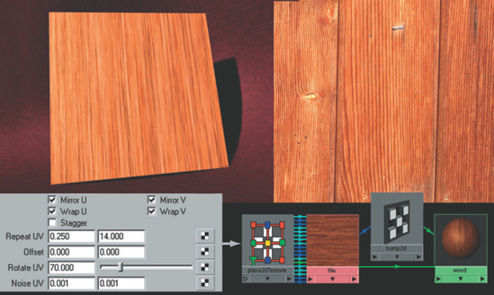
Figure 4.31. (Top left) 3D wood. (Top right) Reference photo of wood. (Bottom) Wood shading network. This scene is included on the CD as wood.ma.
The Blinn has the following custom settings:
Diffuse | 0.95 |
Eccentricity | 0.35 |
Specular Roll Off | 0.22 |
Specular Color | light orange |
The File texture's 2D Placement utility has the following custom settings:
Mirror U | On |
Mirror V | On |
Repeat UV | 0.25, 14 |
Rotate UV | 70 |
Noise UV | 0.001, 0.001 |
The Noise UV attribute creates subtle distortions in the File texture, making the texture repeat less obvious. The Mirror U and Mirror V attributes flip the texture each time it's repeated, adding even more variety. In addition, the Color Gain of File texture is tinted brown. The Filter Offset of the File is set to 0.02, which softens the texture slightly. The File texture is also applied as a bump map. The Bump 2D utility's Bump Depth value is set to 0.005.
Note
If Noise UV is raised above 0, 0, the only Filter Type available to the renderer is Mipmap.
Metal is perhaps the most difficult surface to re-create. Chrome, polished silver, stainless steel, and similar metals can be reproduced with raytraced reflections. (See Chapter 11 for raytracing tips.) Many metal finishes, however, do not create coherent reflections. In such a situation, believability comes from the metal's color and the contrast of the metal to its specular highlight. For instance, cast iron is a very "dark" metal. Although iron has a moderately bright secular highlight, the section of the surface that does not receive direct light becomes dark quickly. In this situation, the iron is a poor light reflector. You can create this look by creating a dark surface color with a diffuse specular highlight. For example, in Figure 4.32 a Blinn material is assigned to a torus with the following custom settings:
Diffuse | 0.09 |
Eccentricity | 0.47 |
Specular Roll Off | 0.5 |
Reflectivity | 0.25 |
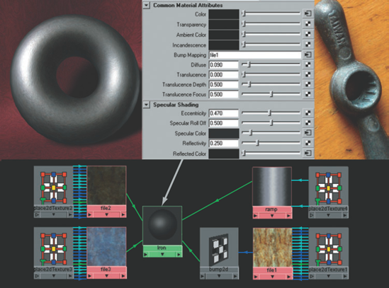
Figure 4.32. (Top left) 3D iron. (Top middle) Blinn material settings. (Top right) Reference photo of iron. (Bottom) Iron shading network. This scene is included on the CD as iron.ma.
The rusty.tif file is loaded into three File textures. The first File (file1) is mapped to the Bump Mapping attribute of the Blinn material (named Iron). The Bump 2D utility's Bump Depth value is set to 0.01, creating a subtle roughness to the surface. The Placement 2D utility for file1 has its Repeat UV set to 2, 1. The second File texture (file2) is mapped to the Blinn's Color. The Color Gain of file2 is lowered to darken the bitmap and thereby reduce the contrast visible as a color. When a File texture is mapped to the Blinn's Color, more variation is present in the render than could be provided by a solid color. The third File (file3) is mapped to the Blinn's Reflected Color. The Reflected Color attribute creates the illusion of reflection without the need to raytrace. The Filter Offset of file3 is set to 0.5, blurring the bitmap. The Invert attribute of file3 is checked, thereby tinting the surface color blue and reducing the contrast. With these settings, the Reflected Color attribute creates a subtle, bluish ambient reflection across the surface. The Reflectivity attribute controls the strength of the Reflected Color effect. Last, a Ramp texture is mapped to the Specular Color of the Blinn. The Ramp has the following custom settings:
Type | U Ramp |
Interpolation | Smooth |
Noise | 0.017 |
Noise Freq | 1.25 |
The Ramp has five handles running from black to light gray. This creates a light band across the center of the torus.
Plastic should never be thought of as a solid color. Even the most finely manufactured plastic product will contain numerous surface imperfections and variations in the specularity. The quickest way to emulate dark plastic is to apply a bitmap as a bump and a specular color. For example, in Figure 4.33 rusty.tif is loaded into a File texture (named file1). The Color Offset of file1 is set to a light blue, which reduces the bitmap's contrast; file1 is mapped to the Specular Color attribute of a Blinn material (named Plastic), which is assigned to a sphere.
The 2D Placement utility for file1 has the following custom settings:
Repeat UV | 40, 40 |
Noise UV | 0.1, 0.2 |
Stagger | On |
The combination of a high Repeat UV value with a relatively high Noise UV value creates very small, near-random detail. Stagger, when checked, offsets each repeat by the half-length of the texture, creating an even more uneven pattern. rusty.tif is also loaded into a second File texture (file2), which is mapped to the Bump Mapping attribute of the Blinn. The Bump 2D utility's Bump Depth is set to 0.01. The 2D Placement utility of file2 also has a high Repeat UV value of 20, 20, a Noise UV value of 0, 0.005, and a Rotate UV value of 90. Last, the Color of the Blinn itself is set a dark gray. The Blinn has the following custom settings:
Diffuse | 0.52 |
Eccentricity | 0.34 |
Specular Roll Off | 0.24 |

Figure 4.33. (Top left) 3D plastic. (Top right) Reference photo of plastic. (Bottom) Plastic shading network. This scene is included on the CD as plastic.ma.
Note
Highly repeated texture maps, such as those described in the previous example, can lead to buzzing and other anti-aliasing problems. The trick is to keep the Repeat UV value as low as possible while maintaining the correct look. A proper Repeat UV value depends on the camera placement, how the surface is lit, if the surface and/or camera is animated, and if motion blur is present. For an additional discussion on anti-aliasing issues, see Chapter 10.
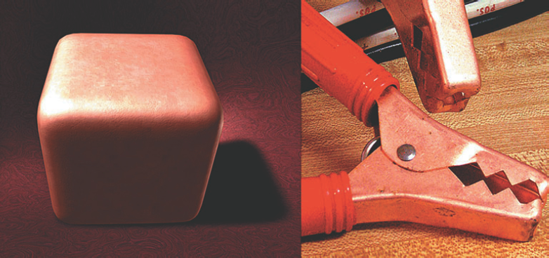
In this tutorial, you will re-create the look of copper with basic texturing techniques. You will use a generic noisy bitmap (rusty.tif) as a color and bump map for a Blinn material.
Copper is a "bright" metal and is highly reflective. If copper has not been polished, however, it creates a highly diffuse reflection. This is due to numerous, microscopic imperfections. Unpolished copper is therefore slightly "glowy" and has an unfocused specular highlight (see Figure 4.34).
Note
Open
copper.mafrom the Chapter 4 scene folder on the CD.Open the Hypershade window. MMB-drag a Blinn material into the work area and rename name it Copper. Assign Copper to the polygon cube.
Open Copper's Attribute Editor tab. Set the Color attribute to a semidark, reddish brown. Use Figure 4.35 as reference. Set the Ambient Color attribute to a lighter reddish brown. A high Ambient Color value replicates the bright quality of the metal. Set Diffuse to 0.7, Eccentricity to 0.49, Specular Roll Off to 0.85, and Reflectivity to 0.15. This combination of settings creates an intense specular highlight that spreads over the edge of the cube without overexposing the top face. Render a test frame. Adjust the Color and Ambient Color attributes to emulate the distinctive copper look.
Click the Bump Mapping attribute's checkered Map button. Click the File button in the Create Render Node window. The Bump 2D utility appears in the Attribute Editor. Set the Bump Depth attribute to −0.003.
In the work area, select the newly created File texture and rename it File1. Click the file browse button beside the Image Name attribute and retrieve
rusty.tiffrom the Chapter 4 texture folder on the CD. In the work area, select the 2D Placement utility (now named place2dTexture1) connected to File1 and open its Attribute Editor tab. Set Repeat UV to 3, 3 and check Stagger. Custom UV settings ensure that the scale of the texture detail is appropriate for the model. Render a test frame.Select Copper and open its Attribute Editor tab. Click the Reflected Color attribute's checkered Map button. Click the File texture button in the Create Render Node window. The new File texture appears in the work area with a 2D Placement utility. Rename the new File texture File2. Click the file browse button beside the Image Name attribute and retrieve
rusty.tiffrom the Chapter 4 texture folder on the CD. Set File2's Filter Offset to 0.005. The Filter Offset value will blur the texture and resulting simulated reflection. The strength of the reflection is controlled by Copper's Reflectivity. The simulated reflection is most noticeable in the dark front face of the cube. Render a test frame.Open Copper's Attribute Editor tab. Click the Specular Color attribute's checkered Map button. Click the File button in the Create Render Node window. The new File texture appears in the work area with a 2D Placement utility. Rename the new File texture File3. Set File3's Filter Offset to 0.005. Change the Color Gain attribute to an RGB value of 66, 62, 72. You can enter color values by clicking the Color Gain color swatch and opening the Color Chooser window (set the color space drop-down to RGB and the color range drop-down to "0 to 255"). This tints the Color Gain with a washed-out lavender, which balances the red of Copper's Color and Ambient Color and creates a copperlike look. Change the Color Offset attribute to a 50 percent gray.
Render a test frame. If the material's color does not look correct, change Copper's Color attribute to an RGB value of 82, 44, 35 and the Ambient Color attribute to an RGB value of 116, 48, 38.
In the work area, select the newest 2D Placement utility (now named place2dTexture3) connected to File3 and open its Attribute Editor tab. Set Repeat UV to 2, 2 and check Stagger. The copper material is complete! If you get stuck, a finished version is saved as
copper_finished.main the Chapter 4 scene folder.