CHAPTER 18
Complex Analysis and Potential Theory

In Chapter 17 we developed the geometric approach of conformal mapping. This meant that, for a complex analytic function w = f(z) defined in a domain D of the z-plane, we associated with each point in D a corresponding point in the w-plane. This gave us a conformal mapping (angle-preserving), except at critical points where f′(z) = 0.
Now, in this chapter, we shall apply conformal mappings to potential problems. This will lead to boundary value problems and many engineering applications in electrostatics, heat flow, and fluid flow. More details are as follows.
Recall that Laplace's equation ∇2Φ = 0 is one of the most important PDEs in engineering mathematics because it occurs in gravitation (Secs. 9.7, 12.11), electrostatics (Sec. 9.7), steady-state heat conduction (Sec. 12.5), incompressible fluid flow, and other areas. The theory of this equation is called potential theory (although “potential” is also used in a more general sense in connection with gradients (see Sec. 9.7)). Because we want to treat this equation with complex analytic methods, we restrict our discussion to the “two-dimensional case.” Then Φ depends only on two Cartesian coordinates x and y, and Laplace's equation becomes
![]()
An important idea then is that its solutions Φ are closely related to complex analytic functions Φ + iΨ as shown in Sec. 13.4. (Remark: We use the notation Φ + iΨ to free u and v, which will be needed in conformal mapping u + iv.) This important relation is the main reason for using complex analysis in problems of physics and engineering.
We shall examine this connection between Laplace's equation and complex analytic functions and illustrate it by modeling applications from electrostatics (Secs. 18.1, 18.2), heat conduction (Sec. 18.3), and hydrodynamics (Sec. 18.4). This in turn will lead to boundary value problems in two-dimensional potential theory. As a result, some of the functions of Chap. 17 will be used to transform complicated regions into simpler ones.
Section 18.5 will derive the important Poisson formula for potentials in a circular disk. Section 18.6 will deal with harmonic functions, which, as you recall, are solutions of Laplace's equation and have continuous second partial derivatives. In that section we will show how results on analytic functions can be used to characterize properties of harmonic functions.
Prerequisite: Chaps. 13, 14, 17.
References and Answers to Problems: App. 1 Part D, App. 2.
18.1 Electrostatic Fields
The electrical force of attraction or repulsion between charged particles is governed by Coulomb's law (see Sec. 9.7). This force is the gradient of a function Φ, called the electrostatic potential. At any points free of charges, Φ is a solution of Laplace's equation
![]()
The surfaces Φ = const are called equipotential surfaces. At each point P at which the gradient of Φ is not the zero vector, it is perpendicular to the surface Φ = const through P; that is, the electrical force has the direction perpendicular to the equipotential surface. (See also Secs. 9.7 and 12.11.)
The problems we shall discuss in this entire chapter are two-dimensional (for the reason just given in the chapter opening), that is, they model physical systems that lie in three-dimensional space (of course!), but are such that the potential Φ is independent of one of the space coordinates, so that Φ depends only on two coordinates, which we call x and y. Then Laplace's equation becomes

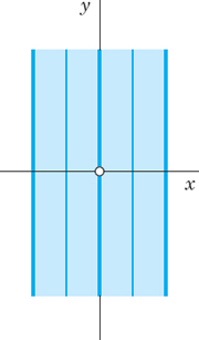
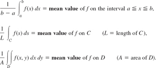
Fig. 396. Potential in Example 1
Equipotential surfaces now appear as equipotential lines (curves) in the xy-plane.
Let us illustrate these ideas by a few simple examples.
EXAMPLE 1 Potential Between Parallel Plates
Find the potential Φ of the field between two parallel conducting plates extending to infinity (Fig. 396), which are kept at potentials Φ1 and Φ2, respectively.
Solution. From the shape of the plates it follows that Φ depends only on x, and Laplace's equation becomes Φ″ = 0. By integrating twice we obtain Φ = ax + b, where the constants a and b are determined by the given boundary values of Φ on the plates. For example, if the plates correspond to x = −1 and x = 1, the solution is
![]()
The equipotential surfaces are parallel planes.
EXAMPLE 2 Potential Between Coaxial Cylinders
Find the potential Φ between two coaxial conducting cylinders extending to infinity on both ends (Fig. 397) and kept at potentials Φ1 and Φ2, respectively.
Solution. Here Φ depends only on ![]() for reasons of symmetry, and Laplace's equation r2urr + rur + uθθ = 0 [(5), Sec. 12.10] with uθθ = 0 and u = Φ becomes rΦ″ + Φ′ = 0. By separating variables and integrating we obtain
for reasons of symmetry, and Laplace's equation r2urr + rur + uθθ = 0 [(5), Sec. 12.10] with uθθ = 0 and u = Φ becomes rΦ″ + Φ′ = 0. By separating variables and integrating we obtain
![]()
and a and b are determined by the given values of Φ on the cylinders. Although no infinitely extended conductors exist, the field in our idealized conductor will approximate the field in a long finite conductor in that part which is far away from the two ends of the cylinders.

Fig. 397. Potential in Example 2
EXAMPLE 3 Potential in an Angular Region
Find the potential Φ between the conducting plates in Fig. 398, which are kept at potentials Φ1 (the lower plate) and Φ2, and make an angle α, where 0 < α ![]() π. (In the figure we have α = 120° = 2π/3
π. (In the figure we have α = 120° = 2π/3
Solution. θ = Arg z (z = x + iy ≠ 0) is constant on rays θ = const. It is harmonic since it is the imaginary part of an analytic function, Ln z (Sec. 13.7). Hence the solution is
![]()
with a and b determined from the two boundary conditions (given values on the plates)
![]()
Thus a = (Φ2 + Φ1)/2, b = (Φ2 − Φ1)/α. The answer is
![]()

Fig. 398. Potential in Example 3
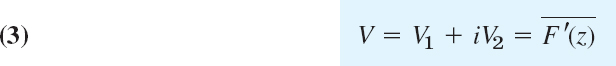
Complex Potential
Let Φ (x, y) be harmonic in some domain D and Ψ(x, y) a harmonic conjugate of Ψ in D. (Note the change of notation from u and v of Sec. 13.4 to Φ and Ψ. From the next section on, we had to free u and v for use in conformal mapping. Then

is an analytic function of z = x + iy. This function F is called the complex potential corresponding to the real potential Φ. Recall from Sec. 13.4 that for given Φ, a conjugate Ψ is uniquely determined except for an additive real constant. Hence we may say the complex potential, without causing misunderstandings.
The use of F has two advantages, a technical one and a physical one. Technically, F is easier to handle than real or imaginary parts, in connection with methods of complex analysis. Physically, Ψ has a meaning. By conformality, the curves Ψ = const intersect the equipotential lines Φ = const in the xy-plane at right angles [except where F′(z) = 0]. Hence they have the direction of the electrical force and, therefore, are called lines of force. They are the paths of moving charged particles (electrons in an electron microscope, etc.).
In Example 1, a conjugate is Ψ = ay. It follows that the complex potential is
![]()
and the lines of force are horizontal straight lines y = const parallel to the x-axis.
In Example 2 we have Φ = a ln + r + b = a ln |z| + b. A conjugate is Ψ = a Arg z. Hence the complex potential is
![]()
and the lines of force are straight lines through the origin. F(z) may also be interpreted as the complex potential of a source line (a wire perpendicular to the xy-plane) whose trace in the xy-plane is the origin.
In Example 3 we get F(z) by noting that i Ln z = i ln |z| − Arg z, multiplying this by −b, and adding a:
![]()
We see from this that the lines of force are concentric circles |z| = const. Can you sketch them?
Superposition
More complicated potentials can often be obtained by superposition.
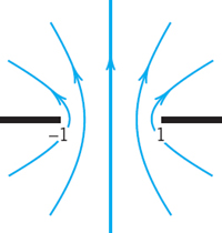
EXAMPLE 7 Potential of a Pair of Source Lines (a Pair of Charged Wires)
Determine the potential of a pair of oppositely charged source lines of the same strength at the points z = c and z = −c on the real axis.
Solution. From Examples 2 and 5 it follows that the potential of each of the source lines is
![]()
respectively. Here the real constant K measures the strength (amount of charge). These are the real parts of the complex potentials
![]()
Hence the complex potential of the combination of the two source lines is
![]()
The equipotential lines are the curves
![]()
These are circles, as you may show by direct calculation. The lines of force are
![]()
We write this briefly (Fig. 399)
![]()
Now θ1 − θ2 is the angle between the line segments from z to c and −c (Fig. 399). Hence the lines of force are the curves along each of which the line segment S: −c ![]() x
x ![]() c appears under a constant angle. These curves are the totality of circular arcs over S, as is (or should be) known from elementary geometry. Hence the lines of force are circles. Figure 400 shows some of them together with some equipotential lines.
c appears under a constant angle. These curves are the totality of circular arcs over S, as is (or should be) known from elementary geometry. Hence the lines of force are circles. Figure 400 shows some of them together with some equipotential lines.
In addition to the interpretation as the potential of two source lines, this potential could also be thought of as the potential between two circular cylinders whose axes are parallel but do not coincide, or as the potential between two equal cylinders that lie outside each other, or as the potential between a cylinder and a plane wall. Explain this using Fig. 400.
The idea of the complex potential as just explained is the key to a close relation of potential theory to complex analysis and will recur in heat flow and fluid flow.
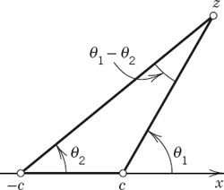
Fig. 399. Arguments in Example 7

Fig. 400. Equipotential lines and lines of force (dashed) in Example 7
1–4 COAXIAL CYLINDERS
Find and sketch the potential between two coaxial cylinders of radii r1 and r2 having potential U1 and U2, respectively.
- r1 = 2.5 mm, r2 = 4.0 cm, U1 = 0 V, U2 = 220 V
- r1 = 1 cm, r2 = 2 cm, U1 = 400 V, U2 = 0 V
- r1 = 10 cm, r2 = 1 m, U1 = 10 kV, U2 = −10 kV
- If r1 = 2 cm, r2 = 6 cm and U1 = 300 V, U2 = 100 V, respectively, is the potential at r = 4 cm equal to 200 V? Less? More? Answer without calculation. Then calculate and explain.
5–7 PARALLEL PLATES
Find and sketch the potential between the parallel plates having potentials U1 and U2. Find the complex potential.
- 5. Plates at x1 = −5 cm, x2 = 5 cm, potentials U1 = 250 V, U2 = 500 V, respectively.
- 6. Plates at y = x and y = x + k, potentials U1 = 0V, U2 = 220 V, respectively.
- 7. Plates at x1 = 12 cm, x2 = 24 cm, potentials U1 = 20 kV, U2 = 8 kV, respectively.
- 8. CAS EXPERIMENT. Complex Potentials. Graph the equipotential lines and lines of force in (a)–(d) (four graphs, Re F(z) and Im F(z) on the same axes). Then explore further complex potentials of your choice with the purpose of discovering configurations that might be of practical interest.
- F(z) = z2
- F(z) = iz2
- F(z) = 1/z
- F(z) = i/z
- 9. Argument. Show that Φ = θ/π = (1/π) arctan (y/x) is harmonic in the upper half-plane and satisfies the boundary condition Φ(x, 0) = 1 if x < 0 and 0 if x > 0, and the corresponding complex potential is F(z) = −(i/π)Ln z.
- 10. Conformal mapping. Map the upper z-half-plane onto |w|
 1 so that 0, ∞, −1 are mapped onto 1, i, −i, respectively. What are the boundary conditions on |w| = 1 resulting from the potential in Prob. 9? What is the potential at w = 0?
 - 11. Text Example 7. Verify, by calculation, that the equipotential lines are circles.
12–15 OTHER CONFIGURATIONS
- 12. Find and sketch the potential between the axes (potential 500 V) and the hyperbola xy = 4 (potential 100 V).
- 13. Arccos. Show that F(z) = arccos z (defined in Problem Set 13.7) gives the potential of a slit in Fig. 401.

- 14. Arccos. Show that F(z) in Prob. 13 gives the potentials in Fig. 402.

- 15. Sector. Find the real and complex potentials in the sector −π/6 θ π/6 between the boundary θ = ±π/6, kept at 0 V, and the curve x3 − 3xy2 = 1, kept at 220 V.
18.2 Use of Conformal Mapping. Modeling
We have just explored the close relation between potential theory and complex analysis. This relationship is so close because complex potentials can be modeled in complex analysis. In this section we shall explore the close relation that results from the use of conformal mapping in modeling and solving boundary value problems for the Laplace equation. The process consists of finding a solution of the equation in some domain, assuming given values on the boundary (Dirichlet problem, see also Sec. 12.6). The key idea is then to use conformal mapping to map a given domain onto one for which the solution is known or can be found more easily. This solution thus obtained is then mapped back to the given domain. The reason this approach works is due to Theorem 1, which asserts that harmonic functions remain harmonic under conformal mapping:
THEOREM 1 Harmonic Functions Under Conformal Mapping
Let Φ* be harmonic in a domain D* in the w-plane. Suppose that w = u + iv = f(z) is analytic in a domain D in the z-plane and maps D conformally onto D*. Then the function
![]()
is harmonic in D.
PROOF
The composite of analytic functions is analytic, as follows from the chain rule. Hence, taking a harmonic conjugate Ψ*(u, v) of Φ*, as defined in Sec. 13.4, and forming the analytic function F*(w) = Φ*(u, v) + iΨ*(u, v) we conclude that F(z) = F*(f(z)) is analytic in D. Hence its real part Φ(x, y) = Re F(z) is harmonic in D. This completes the proof.
We mention without proof that if D* is simply connected (Sec. 14.2), then a harmonic conjugate of Φ* exists. Another proof of Theorem 1 without the use of a harmonic conjugate is given in App. 4.
EXAMPLE 1 Potential Between Noncoaxial Cylinders
Model the electrostatic potential between the cylinders C1: |z| = 1 and ![]() in Fig. 403. Then give the solution for the case that C1 is grounded, U1 = 0 V, and C2 has the potential U2 = 110 V.
in Fig. 403. Then give the solution for the case that C1 is grounded, U1 = 0 V, and C2 has the potential U2 = 110 V.
Solution. We map the unit disk |z| = 1 onto the unit disk |w| = 1 in such a way that C2 is mapped onto some cylinder ![]() By (3), Sec. 17.3, a linear fractional transformation mapping the unit disk onto the unit disk is
By (3), Sec. 17.3, a linear fractional transformation mapping the unit disk onto the unit disk is


Fig. 403. Example 1: z-plane
Fig. 404. Example 1: w-plane
where we have chosen b = z0 real without restriction. z0 is of no immediate help here because centers of circles do not map onto centers of the images, in general. However, we now have two free constants b and r0 and shall succeed by imposing two reasonable conditions, namely, that 0 and ![]() (Fig. 403) should be mapped onto r0 and −r0 (Fig. 404), respectively. This gives by (2)
(Fig. 403) should be mapped onto r0 and −r0 (Fig. 404), respectively. This gives by (2)

a quadratic equation in r0 with solutions r0 = 2 (no good because r0 < 1) and ![]() Hence our mapping function (2) with
Hence our mapping function (2) with ![]() becomes that in Example 5 of Sec. 17.3,
becomes that in Example 5 of Sec. 17.3,

From Example 5 in Sec. 18.1, writing w for z we have as the complex potential in the w-plane the function F*(w) = a Ln w + k and from this the real potential
![]()
This is our model. We now determine a and k from the boundary conditions. If |w| = 1, then Φ* = a ln 1 + k = 0, hence k = 0. If ![]() then Φ* = a ln
then Φ* = a ln ![]() hence a = 110/ln
hence a = 110/ln ![]() Substitution of (3) now gives the desired solution in the given domain in the z-plane
Substitution of (3) now gives the desired solution in the given domain in the z-plane

The real potential is

Can we “see” this result? Well, Φ(x, y) = const if and only if |(2z − 1)/(z − 2)| = const, that is, |w| = const by (2) with ![]() . These circles are images of circles in the z-plane because the inverse of a linear fractional transformation is linear fractional (see (4), Sec. 17.2), and any such mapping maps circles onto circles (or straight lines), by Theorem 1 in Sec. 17.2. Similarly for the rays arg w = const. Hence the equipotential lines Φ(x, y) = const are circles, and the lines of force are circular arcs (dashed in Fig. 404). These two families of curves intersect orthogonally, that is, at right angles, as shown in Fig. 404.
. These circles are images of circles in the z-plane because the inverse of a linear fractional transformation is linear fractional (see (4), Sec. 17.2), and any such mapping maps circles onto circles (or straight lines), by Theorem 1 in Sec. 17.2. Similarly for the rays arg w = const. Hence the equipotential lines Φ(x, y) = const are circles, and the lines of force are circular arcs (dashed in Fig. 404). These two families of curves intersect orthogonally, that is, at right angles, as shown in Fig. 404.
EXAMPLE 2 Potential Between Two Semicircular Plates
Model the potential between two semicircular plates P1 and P2 in Fig. 405 having potentials −3000 V and 3000 V, respectively. Use Example 3 in Sec. 18.1 and conformal mapping.
Solution. Step 1. We map the unit disk in Fig. 405 onto the right half of the w-plane (Fig. 406) by using the linear fractional transformation in Example 3, Sec. 17.3:


Fig. 405. Example 2: z-plane

Fig. 406. Example 2: w-plane
The boundary |z| = 1 is mapped onto the boundary u = 0 (the v-axis), with z = −1, i, 1 going onto w = 0, i, ∞, respectively, and z = −i onto w = −i. Hence the upper semicircle of |z| = 1 is mapped onto the upper half, and the lower semicircle onto the lower half of the v-axis, so that the boundary conditions in the w-plane are as indicated in Fig. 406.
Step 2. We determine the potential Φ*(u, v) in the right half-plane of the w-plane. Example 3 in Sec. 18.1 with α = π, U1 = −3000, and U2 = 3000 [with Φ*(u, v) instead of Φ(x, y)] yields
![]()
On the positive half of the imaginary axis (φ = π/2), this equals 3000 and on the negative half −3000, as it should be. Φ* is the real part of the complex potential
![]()
Step 3. We substitute the mapping function into F* to get the complex potential F(z) in Fig. 405 in the form
![]()
The real part of this is the potential we wanted to determine:
![]()
As in Example 1 we conclude that the equipotential lines Φ(x, y) = const are circular arcs because they correspond to Arg [(1 + z)/(1 − z)] = const, hence to Arg w = const. Also, Arg w = const are rays from 0 to ∞, the images of z = −1 and z = 1, respectively. Hence the equipotential lines all have −1 and 1 (the points where the boundary potential jumps) as their endpoints (Fig. 405). The lines of force are circular arcs, too, and since they must be orthogonal to the equipotential lines, their centers can be obtained as intersections of tangents to the unit circle with the x-axis, (Explain!)
Further examples can easily be constructed. Just take any mapping w = f(z) in Chap. 17, a domain D in the z-plane, its image D* in the w-plane, and a potential Φ* in D*. Then (1) gives a potential in D. Make up some examples of your own, involving, for instance, linear fractional transformations.
Basic Comment on Modeling
We formulated the examples in this section as models on the electrostatic potential. It is quite important to realize that this is accidental. We could equally well have phrased everything in terms of (time-independent) heat flow; then instead of voltages we would have had temperatures, the equipotential lines would have become isotherms (= lines of constant temperature), and the lines of the electrical force would have become lines along which heat flows from higher to lower temperatures (more on this in the next section). Or we could have talked about fluid flow; then the electrostatic lines of force would have become streamlines (more on this in Sec. 18.4). What we again see here is the unifying power of mathematics: different phenomena and systems from different areas in physics having the same types of model can be treated by the same mathematical methods. What differs from area to area is just the kinds of problems that are of practical interest.
- Derivation of (3) from (2). Verify the steps.
- Second proof. Give the details of the steps given on p. A93 of the book. What is the point of that proof?
3–5 APPLICATION OF THEOREM 1
- 3. Find the potential Φ in the region R in the first quadrant of the z-plane bounded by the axes (having potential U1) and the hyperbola y = 1/x (having potential U2) by mapping R onto a suitable infinite strip. Show that Φ is harmonic. What are its boundary values?
- 4. Let Φ* = 4uv, w = f(z) = ez, and D: x < 0, 0 < y < π. Find Φ. What are its boundary values?
- 5. CAS PROJECT. Graphing Potential Fields. Graph equipotential lines (a) in Example 1 of the text, (b) if the complex potential is F(z) = z2, iz2, ez. (c) Graph the equipotential surfaces for F(z) = Ln z as cylinders in space.
- 6. Apply Theorem 1 to Φ*(u, v) = u2 − v2, w = f(z) = ez, and any domain D, showing that the resulting potential Φ is harmonic.
- 7. Rectangle, sin z. Let D:
 , 0 y 1; D* the image of D under w = sin z; and Φ* = u2 − v2. What is the corresponding potential Φ in D? What are its boundary values? Sketch D and D*.
 - 8. Conjugate potential. What happens in Prob. 7 if you replace the potential by its conjugate harmonic?
- 9. Translation. What happens in Prob. 7 if we replace by sin z by
 ?
? - 10. Noncoaxial Cylinders. Find the potential between the cylinders C1: |z| = 1 (potential U1 = 0) and C2: |z − c| = c (potential U2 = 220 V), where 0 < c <
 . Sketch or graph equipotential lines and their orthogonal trajectories for
  Can you guess how the graph changes if you increase
  ?
? - 11. On Example 2. Verify the calculations.
- 12. Show that in Example 2 the y-axis is mapped onto the unit circle in the w-plane.
- 13. At z = ±1 in Fig. 405 the tangents to the equipotential lines as shown make equal angles. Why?
- 14. Figure 405 gives the impression that the potential on the y-axis changes more rapidly near 0 than near ±i. Can you verify this?
- 15. Angular region. By applying a suitable conformal mapping, obtain from Fig. 406 the potential Φ in the sector
 such that Φ = −3 kV if
  and Φ = 3 kV if .
 - 16. Solve Prob. 15 if the sector is
- 17. Another extension of Example 2. Find the linear fractional transformation z = g(Z) that maps |Z| 1 onto |z| 1 with Z = i/2 being mapped onto z = 0. Show that Z1 = −0.6 + 0.8i is mapped onto z = −1 and Z2 = −0.6 + 0.8i onto z = 1, so that the equipotential lines of Example 2 look in |Z| 1 as shown in Fig. 407.

- 18. The equipotential lines in Prob. 17 are circles. Why?
- 19. Jump on the boundary. Find the complex and real potentials in the upper half-plane with boundary values 5 kV if x < 2 and 0 if x > 2 on the x-axis.
- 20. Jumps. Do the same task as in Prob. 19 if the boundary values on the x-axis are V0 when −a < x < a and 0 elsewhere.
18.3 Heat Problems
Heat conduction in a body of homogeneous material is modeled by the heat equation
![]()
where the function T is temperature, Tt = ∂T/∂t, t is time, and c2 is a positive constant (specific to the material of the body; see Sec. 12.6).
Now if a heat flow problem is steady, that is, independent of time, we have Tt = 0. If it is also two-dimensional, then the heat equation reduces to
![]()
which is the two-dimensional Laplace equation. Thus we have shown that we can model a two-dimensional steady heat flow problem by Laplace's equation.
Furthermore we can treat this heat flow problem by methods of complex analysis, since T (or T(x, y)) is the real part of the complex heat potential
![]()
We call T(x, y) the heat potential. The curves T(x, y) = const are called isotherms, which means lines of constant temperature. The curves Ψ(x, y) = const are called heat flow lines because heat flows along them from higher temperatures to lower temperatures.
It follows that all the examples considered so far (Secs. 18.1, 18.2) can now be reinterpreted as problems on heat flow. The electrostatic equipotential lines Φ(x, y) = const now become isotherms T(x, y) = const, and the lines of electrical force become lines of heat flow, as in the following two problems.
EXAMPLE 1 Temperature Between Parallel Plates
Find the temperature between two parallel plates x = 0 and x = d in Fig. 408 having temperatures 0 and 100°C, respectively.
Solution. As in Example 1 of Sec. 18.1 we conclude that T(x, y) = ax + b. From the boundary conditions, b = 0 and a = 100/d. The answer is
![]()
The corresponding complex potential is F(z) = (100/d)z. Heat flows horizontally in the negative x-direction along the lines y = const.
EXAMPLE 2 Temperature Distribution Between a Wire and a Cylinder
Find the temperature field around a long thin wire of radius r1 = 1 mm that is electrically heated to T1 = 500°F and is surrounded by a circular cylinder of radius r2 = 100 mm, which is kept at temperature T2 = 60°F by cooling it with air. See Fig. 409. (The wire is at the origin of the coordinate system.)
Solution.T depends only on r, for reasons of symmetry. Hence, as in Sec. 18.1 (Example 2),
![]()
The boundary conditions are
![]()
Hence b = 500 (since ln 1 = 0) and a = (60 − b)/ln 100 = −95.54. The answer is
![]()
The isotherms are concentric circles. Heat flows from the wire radially outward to the cylinder. Sketch T as a function of r. Does it look physically reasonable?

Fig. 408. Example 1

Fig. 409. Example 2

Fig. 410. Example 3
Mathematically the calculations remain the same in the transition to another field of application. Physically, new problems may arise, with boundary conditions that would make no sense physically or would be of no practical interest. This is illustrated by the next two examples.
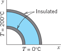
EXAMPLE 3 A Mixed Boundary Value Problem
Find the temperature distribution in the region in Fig. 410 (cross section of a solid quarter-cylinder), whose vertical portion of the boundary is at 20°C, the horizontal portion at 50°C, and the circular portion is insulated.
Solution. The insulated portion of the boundary must be a heat flow line, since, by the insulation, heat is prevented from crossing such a curve, hence heat must flow along the curve. Thus the isotherms must meet such a curve at right angles. Since T is constant along an isotherm, this means that
![]()
Here ∂T/∂n is the normal derivative of T, that is, the directional derivative (Sec. 9.7) in the direction normal (perpendicular) to the insulated boundary. Such a problem in which T is prescribed on one portion of the boundary and ∂T/∂n on the other portion is called a mixed boundary value problem.
In our case, the normal direction to the insulated circular boundary curve is the radial direction toward the origin. Hence (2) becomes ∂T/∂r = 0, meaning that along this curve the solution must not depend on r. Now Arg z = θ satisfies (1), as well as this condition, and is constant (0 and π/2) on the straight portions of the boundary. Hence the solution is of the form
![]()
The boundary conditions yield a · π/2 + b = 20 and a · 0 + b = 50. This gives
![]()
The isotherms are portions of rays θ = const. Heat flows from the x-axis along circles r = const (dashed in Fig. 410) to the y-axis.

Fig. 411. Example 4: z-plane
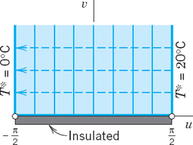
Fig. 412. Example 4: w-plane
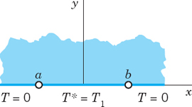
EXAMPLE 4 Another Mixed Boundary Value Problem in Heat Conduction
Find the temperature field in the upper half-plane when the x-axis is kept at T = 0°C for x < −1, is insulated for −1 < x < 1, and is kept at T = 20°C for x > 1 (Fig. 411).
Solution. We map the half-plane in Fig. 411 onto the vertical strip in Fig. 412, find the temperature T*(u, v) there, and map it back to get the temperature T(x, y) in the half-plane.
The idea of using that strip is suggested by Fig. 391 in Sec. 17.4 with the roles of z = x + iy and w = u + iv interchanged. The figure shows that z = sin w maps our present strip onto our half-plane in Fig. 411. Hence the inverse function
![]()
maps that half-plane onto the strip in the w-plane. This is the mapping function that we need according to Theorem 1 in Sec. 18.2.
The insulated segment −1 < x < 1 on the x-axis maps onto the segment −π/2 < u < π/2 on the u-axis. The rest of the x-axis maps onto the two vertical boundary portions u = −π/2 and π/2, v > 0, of the strip. This gives the transformed boundary conditions in Fig. 412 for T*(u, v), where on the insulated horizontal boundary, ∂T*/∂n = ∂T*/∂v = 0 because v is a coordinate normal to that segment.
Similarly to Example 1 we obtain
![]()
which satisfies all the boundary conditions. This is the real part of the complex potential F*(w) = 10 + (20/π)w. Hence the complex potential in the z-plane is
![]()
and T(x, y) = Re F(z) is the solution. The isotherms are u = const in the strip and the hyperbolas in the z-plane, perpendicular to which heat flows along the dashed ellipses from the 20°-portion to the cooler 0°-portion of the boundary, a physically very reasonable result.
Sections 18.3 and 18.5 show some of the usefulness of conformal mappings and complex potentials. Furthermore, complex potential models fluid flow in Sec. 18.4.
- Parallel plates. Find the temperature between the plates y = 0 and y = d kept at 20 and 100°C, respectively. (i) Proceed directly. (ii) Use Example 1 and a suitable mapping.
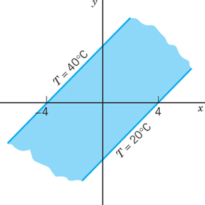
- Infinite plate. Find the temperature and the complex potential in an infinite plate with edges y = x − 4 and y = x + 4 kept at −20 and 40°C, respectively (Fig. 413). In what case will this be an approximate model?
- CAS PROJECT. Isotherms. Graph isotherms and lines of heat flow in Examples 2–4. Can you see from the graphs where the heat flow is very rapid?
4–18 TEMPERATURE T(x, y) IN PLATES
Find the temperature distribution T(x, y) and the complex potential F(z) in the given thin metal plate whose faces are insulated and whose edges are kept at the indicated temperatures or are insulated as shown.
- 4.

- 5.

- 6.

- 7.

- 8.

- 9.
- 10.

- 11.

- 12.
 Hint. Apply w = cosh z to Prob. 11.
 - 13.

- 14.
- 15.

- 16.
- 17. First quadrant of the z-plane with y-axis kept at 100°C, the segment 0 < x < 1 of the x-axis insulated and the x-axis for x > 1 kept at 200°C. Hint. Use Example 4.
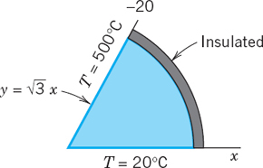
- 18. Figure 410, T(0, y) = −30°C, T(x, 0) = 100°C
- 19. Interpretation. Formulate Prob. 11 in terms of electrostatics.
- 20. Interpretation. Interpret Prob. 17 in Sec. 18.2 as a heat problem, with boundary temperatures, say, 10°C on the upper part and 200°C on the lower.
18.4 Fluid Flow
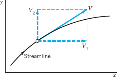
Laplace's equation also plays a basic role in hydrodynamics, in steady nonviscous fluid flow under physical conditions discussed later in this section. For methods of complex analysis to be applicable, our problems will be two-dimensional, so that the velocity vector V by which the motion of the fluid can be given depends only on two space variables x and y, and the motion is the same in all planes parallel to the xy-plane.
Then we can use for the velocity vector V a complex function
![]()
giving the magnitude |V| and direction Arg V of the velocity at each point z = x + iy. Here V1 and V2 are the components of the velocity in the x and y directions. V is tangential to the path of the moving particles, called a streamline of the motion (Fig. 414).
We show that under suitable assumptions (explained in detail following the examples), for a given flow there exists an analytic function

called the complex potential of the flow, such that the streamlines are given by Ψ(x, y) = const, and the velocity vector or, briefly, the velocity is given by
where the bar denotes the complex conjugate. Ψ is called the stream function. The function Φ is called the velocity potential. The curves Φ(x, y) = const are called equipotential lines. The velocity vector V is the gradient of Φ; by definition, this means that

Indeed, for F = Φ + iΨ, Eq. (4) in Sec. 13.4 is F′ = Φx + iΨx with Ψx = −Φy by the second Cauchy–Riemann equation. Together we obtain (3):
![]()
Furthermore, since F(z) is analytic, Φ and Ψ satisfy Laplace's equation

Whereas in electrostatics the boundaries (conducting plates) are equipotential lines, in fluid flow the boundaries across which fluid cannot flow must be streamlines. Hence in fluid flow the stream function is of particular importance.
Before discussing the conditions for the validity of the statements involving (2)–(5), let us consider two flows of practical interest, so that we first see what is going on from a practical point of view. Further flows are included in the problem set.
EXAMPLE 1 Flow Around a Corner
The complex potential F(z) = z2 = x2 − y2 + 2ixy models a flow with

From (3) we obtain the velocity vector
![]()
The speed (magnitude of the velocity) is
![]()
The flow may be interpreted as the flow in a channel bounded by the positive coordinates axes and a hyperbola, say, xy = 1 (Fig. 415). We note that the speed along a streamline S has a minimum at the point P where the cross section of the channel is large.

Fig. 415. Flow around a corner (Example 1)
EXAMPLE 2 Flow Around a Cylinder
Consider the complex potential
![]()
Using the polar form z = reiθ, we obtain

Hence the streamlines are
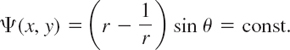
In particular, Ψ(x, y) = 0 gives r − 1/r = 0 or sin θ = 0. Hence this streamline consists of the unit circle (r = 1/r gives r = 1) and the x-axis (θ = 0 and θ = π). For large |z| the term 1/z in F(z) is small in absolute value, so that for these z the flow is nearly uniform and parallel to the x-axis. Hence we can interpret this as a flow around a long circular cylinder of unit radius that is perpendicular to the z-plane and intersects it in the unit circle |z| = 1 and whose axis corresponds to z = 0.
The flow has two stagnation points (that is, points at which the velocity V is zero), at z = ±1. This follows from (3) and
![]()

Fig. 416. Flow around a cylinder (Example 2)
Assumptions and Theory Underlying (2)–(5)
THEOREM 1 Complex Potential of a Flow
If the domain of flow is simply connected and the flow is irrotational and incompressible, then the statements involving (2)–(5) hold. In particular, then the flow has a complex potential F(z), which is an analytic function. (Explanation of terms below.)
PROOF
We prove this theorem, along with a discussion of basic concepts related to fluid flow.
(a) First Assumption: Irrotational. Let C be any smooth curve in the z-plane given by z(s) = x(s) + iy(s), where s is the arc length of C. Let the real variable Vt be the component of the velocity V tangent to C (Fig. 417). Then the value of the real line integral
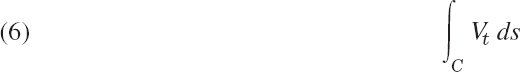

Fig. 417. Tangential component of the velocity with respect to a curve C
taken along C in the sense of increasing s is called the circulation of the fluid along C, a name that will be motivated as we proceed in this proof. Dividing the circulation by the length of C, we obtain the mean velocity1 of the flow along the curve C. Now
![]()
Hence Vt is the dot product (Sec. 9.2) of V and the tangent vector dz/ds of C (Sec. 17.1); thus in (6),

The circulation (6) along C now becomes

As the next idea, let C be a closed curve satisfying the assumption as in Green's theorem (Sec. 10.4), and let C be the boundary of a simply connected domain D. Suppose further that V has continuous partial derivatives in a domain containing D and C. Then we can use Green's theorem to represent the circulation around C by a double integral,
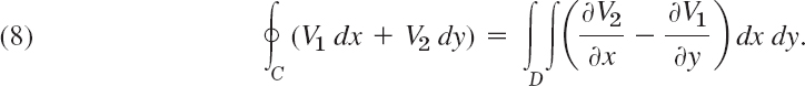
The integrand of this double integral is called the vorticity of the flow. The vorticity divided by 2 is called the rotation

We assume the flow to be irrotational, that is, ω(x, y) ≡ 0 throughout the flow; thus,

To understand the physical meaning of vorticity and rotation, take for C in (8) a circle. Let r be the radius of C. Then the circulation divided by the length 2πr of C is the mean
velocity of the fluid along C. Hence by dividing this by r we obtain the mean angular velocity ω0 of the fluid about the center of the circle:
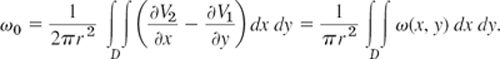
If we now let r → 0, the limit of ω0 is the value of ω at the center of C. Hence ω(x, y) is the limiting angular velocity of a circular element of the fluid as the circle shrinks to the point (x, y). Roughly speaking, if a spherical element of the fluid were suddenly solidified and the surrounding fluid simultaneously annihilated, the element would rotate with the angular velocity ω.
(b) Second Assumption: Incompressible. Our second assumption is that the fluid is incompressible. (Fluids include liquids, which are incompressible, and gases, such as air, which are compressible.) Then
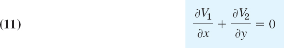
in every region that is free of sources or sinks, that is, points at which fluid is produced or disappears, respectively. The expression in (11) is called the divergence of V and is denoted by div V. (See also (7) in Sec. 9.8.)
(c) Complex Velocity Potential. If the domain D of the flow is simply connected (Sec. 14.2) and the flow is irrotational, then (10) implies that the line integral (7) is independent of path in D (by Theorem 3 in Sec. 10.2, where F1 = V1, F2 = V2, F3 = 0, and z is the third coordinate in space and has nothing to do with our present z). Hence if we integrate from a fixed point (a, b) in D to a variable point (x, y) in D, the integral becomes a function of the point (x, y), say, Φ(x, y):

We claim that the flow has a velocity potential Φ, which is given by (12). To prove this, all we have to do is to show that (4) holds. Now since the integral (7) is independent of path, V1 dx + V2 dy is exact (Sec. 10.2), namely, the differential of Φ, that is,
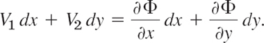
From this we see that V1 = ∂Φ/∂x and V2 = ∂Φ/∂y, which gives (4).
That Φ is harmonic follows at once by substituting (4) into (11), which gives the first Laplace equation in (5).
We finally take a harmonic conjugate Ψ of Φ. Then the other equation in (5) holds. Also, since the second partial derivatives of Φ and Ψ are continuous, we see that the complex function
![]()
is analytic in D. Since the curves Ψ(x, y) = const are perpendicular to the equipotential curves Φ(x, y) = const (except where F′(z) = 0), we conclude that Ψ(x, y) = const are the streamlines. Hence Ψ is the stream function and F(z) is the complex potential of the flow. This completes the proof of Theorem 1 as well as our discussion of the important role of complex analysis in compressible fluid flow.
- Differentiability. Under what condition on the velocity vector V in (1) will F(z) in (2) be analytic?
- Corner flow. Along what curves will the speed in Example 1 be constant? Is this obvious from Fig. 415?
- Cylinder. Guess from physics and from Fig. 416 where on the y-axis the speed is maximum. Then calculate.
- Cylinder. Calculate the speed along the cylinder wall in Fig. 416, also confirming the answer to Prob. 3.
- Irrotational flow. Show that the flow in Example 2 is irrotational.
- Extension of Example 1. Sketch or graph and interpret the flow in Example 1 on the whole upper half-plane.
- Parallel flow. Sketch and interpret the flow with complex potential F(z) = z.
- Parallel flow. What is the complex potential of an upward parallel flow of speed K > 0 in the direction of y = x? Sketch the flow.
- Corner. What F(z) would be suitable in Example 1 if the angle of the corner were π/4 instead of π/2?
- Corner. Show that F(z) = iz2 also models a flow around a corner. Sketch streamlines and equipotential lines. Find V.
- What flow do you obtain from F(z) = −iKz, K positive real?
- Conformal mapping. Obtain the flow in Example 1 from that in Prob. 11 by a suitable conformal mapping.
- 60°- Sector. What F(z) would be suitable in Example 1 if the angle at the corner were π/3?
- Sketch or graph streamlines and equipotential lines of F(z) = iz3. Find V. Find all points at which V is horizontal.
- Change F(z) in Example 2 slightly to obtain a flow around a cylinder of radius r0 that gives the flow in Example 2 if r0 → 1.
- Cylinder. What happens in Example 2 if you replace z by z2? Sketch and interpret the resulting flow in the first quadrant.
- Elliptic cylinder. Show that F(z) = arccos z gives confocal ellipses as streamlines, with foci at z = ±1, and that the flow circulates around an elliptic cylinder or a plate (the segment from −1 to 1 in Fig. 418).

- Aperture. Show that F(z) = arccosh z gives confocal hyperbolas as streamlines, with foci at z = ±1, and the flow may be interpreted as a flow through an aperture (Fig. 419).
- Potential F(z) = 1/z. Show that the streamlines of F(z) = 1/z and circles through the origin with centers on the y-axis.
- TEAM PROJECT. Role of the Natural Logarithm in Modeling Flows. (a) Basic flows: Source and sink. Show that F(z) = (c/2π) ln z with constant positive real c gives a flow directed radially outward (Fig. 420), so that F models a point source at z = 0 (that is, a source line x = 0, y = 0 in space) at which fluid is produced. c is called the strength or discharge of the source. If c is negative real, show that the flow is directed radially inward, so that F models a sink at z = 0, a point at which fluid disappears. Note that z = 0 is the singular point of F(z).
- (b) Basic flows: Vortex. Show that F(z) = −(Ki/2π) ln z with positive real K gives a flow circulating counterclockwise around z = 0 (Fig. 421). z = 0 is called a vortex. Note that each time we travel around the vortex, the potential increases by K.
- (c) Addition of flows. Show that addition of the velocity vectors of two flows gives a flow whose complex potential is obtained by adding the complex potentials of those flows.

- (d) Source and sink combined. Find the complex potentials of a flow with a source of strength 1 at z = −a and of a flow with a sink of strength 1 at z = a. Add both and sketch or graph the streamlines. Show that for small |a| these lines look similar to those in Prob. 19.
- (e) Flow with circulation around a cylinder. Add the potential in (b) to that in Example 2. Show that this gives a flow for which the cylinder wall |z| = 1 is a streamline. Find the speed and show that the stagnation points are
if K = 0 they are at ±1; as K increases they move up on the unit circle until they unite at z = i(K = 4π, see Fig. 422), and if K > 4π they lie on the imaginary axis (one lies in the field of flow and the other one lies inside the cylinder and has no physical meaning).
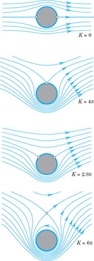
Fig. 422. Flow around a cylinder without circulation (K = 0) and with circulation

18.5 Poisson's Integral Formula for Potentials
So far in this chapter we have seen powerful methods based on conformal mappings and complex potentials. They were used for modeling and solving two-dimensional potential problems and demonstrated the importance of complex analysis.
Now we introduce a further method that results from complex integration. It will yield the very important Poisson integral formula (5) for potentials in a standard domain (a circular disk). In addition, from (5), we will derive a useful series (7) for these potentials. This allows us to solve problems for disks and then map solutions conformally onto other domains.
Derivation of Poisson's Integral Formula
Poisson's formula will follow from Cauchy's integral formula (Sec. 14.3)

Here C is the circle z* = Reiα (counterclockwise, 0 ![]() α
α ![]() 2π), and we assume that F(z*) is analytic in a domain containing C and its full interior. Since dz* = iReiα dα = iz* dα, we obtain from (1)
2π), and we assume that F(z*) is analytic in a domain containing C and its full interior. Since dz* = iReiα dα = iz* dα, we obtain from (1)

Now comes a little trick. If instead of z inside C we take a Z outside C, the integrals (1) and (2) are zero by Cauchy's integral theorem (Sec. 14.2). We choose ![]() which is outside C because |Z| = R2/|z| = R2/r > R. From (2) we thus have
which is outside C because |Z| = R2/|z| = R2/r > R. From (2) we thus have

and by straightforward simplification of the last expression on the right,
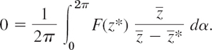
We subtract this from (2) and use the following formula that you can verify by direct calculation (![]() cancels):
cancels):

We then have

From the polar representations of z and z* we see that the quotient in the integrand is real and equal to

We now write F(z) = Φ(r, θ) + iΨ(r, θ) and take the real part on both sides of (4). Then we obtain Poisson's integral formula2
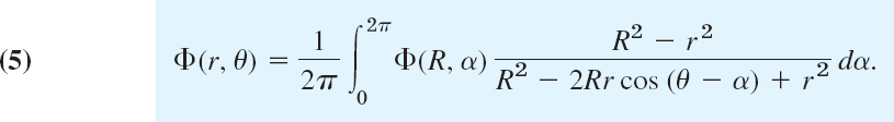
This formula represents the harmonic function Φ in the disk |z| ![]() R in terms of its values Φ(R, α) on the boundary (the circle) |z| = R.
R in terms of its values Φ(R, α) on the boundary (the circle) |z| = R.
Formula (5) is still valid if the boundary function Φ(R, α) is merely piecewise continuous (as is practically often the case; see Figs. 405 and 406 in Sec. 18.2 for an example). Then (5) gives a function harmonic in the open disk, and on the circle |z| = R equal to the given boundary function, except at points where the latter is discontinuous. A proof can be found in Ref. [D1] in App. 1.
Series for Potentials in Disks
From (5) we may obtain an important series development of Φ in terms of simple harmonic functions. We remember that the quotient in the integrand of (5) was derived from (3). We claim that the right side of (3) is the real part of
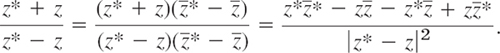
Indeed, the last denominator is real and so is ![]() in the numerator, whereas
in the numerator, whereas ![]() in the numerator is pure imaginary. This verifies our claim. Now by the use of the geometric series we obtain (develop the denominator)
in the numerator is pure imaginary. This verifies our claim. Now by the use of the geometric series we obtain (develop the denominator)

Since z = reiθ and z* = Reiα, we have

On the right, cos(nθ − nα) = cos nθ cos nα + sin nθ sin nα. Hence from (6) we obtain
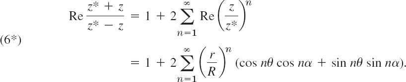
This expression is equal to the quotient in (5), as we have mentioned before, and by inserting it into (5) and integrating term by term with respect to α from 0 to 2π we obtain

where the coefficients are [the 2 in (6*) cancels the 2 in 1/(2π) in (5)]
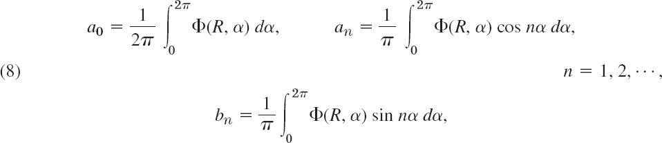
the Fourier coefficients of Φ(R, α); see Sec. 11.1. Now, for r = R, the series (7) becomes the Fourier series of Φ(R, α). Hence the representation (7) will be valid whenever the given Φ(R, α) on the boundary can be represented by a Fourier series.
EXAMPLE 1 Dirichlet Problem for the Unit Disk
Find the electrostatic potential Φ(r, θ) in the unit disk r < 1 having the boundary values
![]()
Solution. Since Φ(1, α) is even, bn = 0, and from (8) we obtain ![]() and
and
![]()
Hence, an = −4/(n2π2) if n is odd, an = 0 if n = 2, 4, …, and the potential is
Figure 424 shows the unit disk and some of the equipotential lines (curves Φ = const).

Fig. 423. Boundary values in Example 1

Fig. 424. Potential in Example 1
- Give the details of the derivation of the series (7) from the Poisson formula (5).
- Verify (3).
- Show that each term of (7) is a harmonic function in the disk r < R.
- Why does the series in Example 1 reduce to a cosine series?
5–18 HARMONIC FUNCTIONS IN A DISK
Using (7), find the potential Φ(r, θ) in the unit disk r < 1 having the given boundary values Φ(1, θ). Using the sum of the first few terms of the series, compute some values of Φ and sketch a figure of the equipotential lines.
- 5.

- 6. Φ(1, θ) = 5 − cos 2θ
- 7. Φ(1, θ) = a cos2 4θ
- 8. Φ(1, θ) = 4 sin3 θ
- 9. Φ(1, θ) = 8 sin4 θ
- 10. Φ(1, θ) = 16 cos32θ
- 11. Φ(1, θ) = θ/π if −π < θ < π
- 12. Φ(1, θ) = k if 0 < θ < π and 0 otherwise
- 13. Φ(1, θ) = θ if
 and 0 otherwise
 - 14. Φ(1, θ) = |θ|/π if −π < θ < π
- 15. Φ(1, θ) = 1 if and 0 otherwise
- 16.

- 17. Φ(1, θ) = θ2/π2 if −π < θ < π
- 18.

- 19. CAS EXPERIMENT. Series (7). Write a program for series developments (7). Experiment on accuracy by computing values from partial sums and comparing them with values that you obtain from your CAS graph. Do this (a) for Example 1 and Fig. 424, (b) for Φ in Prob. 11 (which is discontinuous on the boundary!), (c) for a Φ of your choice with continuous boundary values, and (d) for Φ with discontinuous boundary values.
- 20. TEAM PROJECT. Potential in a Disk. (a) Mean value property. Show that the value of a harmonic function Φ at the center of a circle C equals the mean of the value of Φ on C (see Sec. 18.4, footnote 1, for definitions of mean values).
- (b) Separation of variables. Show that the terms of (7) appear as solutions in separating the Laplace equation in polar coordinates.
- (c) Harmonic conjugate. Find a series for a harmonic conjugate Ψ of Φ from (7). Hint. Use the Cauchy–Riemann equations.
- (d) Power series. Find a series for F(z) = Φ + iΨ.
18.6 General Properties of Harmonic Functions. Uniqueness Theorem for the Dirichlet Problem
Recall from Sec. 10.8 that harmonic functions are solutions to Laplace's equation and their second-order partial derivatives are continuous. In this section we explore how general properties of harmonic functions often can be obtained from properties of analytic functions. This can frequently be done in a simple fashion. Specifically, important mean value properties of harmonic functions follow readily from those of analytic functions. The details are as follows.
THEOREM 1 Mean Value Property of Analytic Functions
Let F(z) be analytic in a simply connected domain D. Then the value of F(z) at a point in D is equal to the mean value of F(z) on any circle in D with center at z0.
In Cauchy's integral formula (Sec. 14.3)
we choose for C the circle z = z0 + reiα in D. Then z − z0 = reiα, dz = ireiα dα, and (1) becomes

The right side is the mean value of F on the circle (= value of the integral divided by the length 2π of the interval of integration). This proves the theorem.
For harmonic functions, Theorem 1 implies
THEOREM 2 Two Mean Value Properties of Harmonic Functions
Let Φ(x, y) be harmonic in a simply connected domain D. Then the value of Φ(x, y) at a point (x0, y0) in D is equal to the mean value of Φ(x, y) on any circle in D with center at (x0, y0). This value is also equal to the mean value of Φ(x, y) on any circular disk in D with center (x0, y0). [See footnote 1 in Sec. 18.4.]
PROOF
The first part of the theorem follows from (2) by taking the real parts on both sides,

The second part of the theorem follows by integrating this formula over r from 0 to r0 (the radius of the disk) and dividing by ![]()

The right side is the indicated mean value (integral divided by the area of the region of integration).
Returning to analytic functions, we state and prove another famous consequence of Cauchy's integral formula. The proof is indirect and shows quite a nice idea of applying the ML-inequality. (A bounded region is a region that lies entirely in some circle about the origin.)
THEOREM 3 Maximum Modulus Theorem for Analytic Functions
Let F(z) be analytic and nonconstant in a domain containing a bounded region R and its boundary. Then the absolute value |F(z)| cannot have a maximum at an interior point of R. Consequently, the maximum of |F(z)| is taken on the boundary of R. If F(z) ≠ 0 in R, the same is true with respect to the minimum of |F(z)|.
We assume that |F(z)| has a maximum at an interior point z0 of R and show that this leads to a contradiction. Let |F(z0)| = M be this maximum. Since F(z) is not constant, |F(z)| is not constant, as follows from Example 3 in Sec. 13.4. Consequently, we can find a circle C of radius r with center at z0 such that the interior of C is in R and |F(z)| smaller than M at some point P of C. Since |F(z)| is continuous, it will be smaller than M on an arc C1 of C that contains P (see Fig. 425), say,
![]()
Let C1 have the length L1. Then the complementary arc C2 of C has the length 2πr − L1. We now apply the ML-inequality (Sec. 14.1) to (1) and note that |z − z0| = r. We then obtain (using straightforward calculation in the second line of the formula)

that is, M < M, which is impossible. Hence our assumption is false and the first statement is proved.
Next we prove the second statement. If F(z) ≠ 0 in R, then 1/F(z) is analytic in R. From the statement already proved it follows that the maximum of 1/|F(z)| lies on the boundary of R. But this maximum corresponds to the minimum of |F(z)|. This completes the proof.

Fig. 425. Proof of Theorem 3
This theorem has several fundamental consequences for harmonic functions, as follows.
Let Φ(x, y) be harmonic in a domain containing a simply connected bounded region R and its boundary curve C. Then:
(I) (Maximum principle) If Φ(x, y) is not constant, it has neither a maximum nor a minimum in R. Consequently, the maximum and the minimum are taken on the boundary of R.
(II) If Φ(x, y) is constant on C, then Φ(x, y) is a constant.
(III) If h(x, y) is harmonic in R and on C and if h(x, y) = Φ(x, y) on C, then h(x, y) = Φ(x, y) everywhere in R.
(I) Let Ψ(x, y) be a conjugate harmonic function of Φ(x, y) in R. Then the complex function F(z) = Φ(x, y) + iΦ(x, y) is analytic in R, and so is G(z) = eF(z). Its absolute value is
![]()
From Theorem 3 it follows that |G(z)| cannot have a maximum at an interior point of R. Since eΦ is a monotone increasing function of the real variable Φ, the statement about the maximum of Φ follows. From this, the statement about the minimum follows by replacing Φ by −Φ.
(II) By (I) the function Φ(x, y) takes its maximum and its minimum on C. Thus, if Φ(x, y) is constant on C, its minimum must equal its maximum, so that Φ(x, y) must be a constant.
(III) If h and Φ are harmonic in R and on C, then h − Φ is also harmonic in R and on C, and by assumption, h − Φ = 0 everywhere on C. By (II) we thus have h − Φ = 0 everywhere in R, and (III) is proved.
The last statement of Theorem 4 is very important. It means that a harmonic function is uniquely determined in R by its values on the boundary of R. Usually, Φ(x, y) is required to be harmonic in R and continuous on the boundary of R, that is,

Under these assumptions the maximum principle (I) is still applicable. The problem of determining Φ(x, y) when the boundary values are given is called the Dirichlet problem for the Laplace equation in two variables, as we know. From (III) we thus have, as a highlight of our discussion,
THEOREM 5 Uniqueness Theorem for the Dirichlet Problem
If for a given region and given boundary values the Dirichlet problem for the Laplace equation in two variables has a solution, the solution is unique.
PROBLEMS RELATED TO THEOREMS 1 AND 2
1–4 Verify Theorem 1 for the given F(z), z0, and circle of radius 1.
- (z + 1)3,

- 2z4, z0 = −2
- (3z − 2)2, z0 = 4
- (z − 1)−2, z0 = −1
- Integrate |z| around the unit circle. Does the result contradict Theorem 1?
- Derive the first statement in Theorem 2 from Poisson's integral formula.
7–9 Verify (3) in Theorem 2 for the given Φ(x, y), (x0, y0), and circle of radius 1.
- 7. (x − 1)(y − 1), (2, −2)
- 8. x2 − y2, (3, 8)
- 9. x + y + xy, (1, 1)
- 10. Verify the calculations involving the inequalities in the proof of Theorem 3.
- 11. CAS EXPERIMENT. Graphing Potentials. Graph the potentials in Probs. 7 and 9 and for two other functions of your choice as surfaces over a rectangle in the xy-plane. Find the locations of the maxima and minima by inspecting these graphs.
- 12. TEAM PROJECT. Maximum Modulus of Analytic Functions. (a) Verify Theorem 3 for (i) F(z) = z2 and the rectangle 1 x 5, 2 y 4, (ii) F(z) = sin z and the unit disk, and (iii) F(z) = ez and any bounded domain.
- (b) F(z) = 1 + |z| is not zero in the disk |z| 2 and has a minimum at an interior point. Does this contradict Theorem 3?
- (c) F(x) = sin x (x real) has a maximum 1 at π/2. Why can this not be a maximum of |F(z)| = |sin z| in a domain containing z = π/2?
- (d) If F(z) is analytic and not constant in the closed unit disk D: |z| 1 and |F(z)| = c = const on the unit circle, show that F(z) must have a zero in D.
- (b) F(z) = 1 + |z| is not zero in the disk |z|
13–17 MAXIMUM MODULUS
Find the location and size of the maximum of |F(z)| in the unit disk |z| ![]() 1.
1.
- 13. F(z) = cos z
- 14. F(z) = exp z2
- 15. F(z) = sinh 2z
- 16. F(z) = az + b (a, b complex, a ≠ 0)
- 17. F(z) = 2z2 − 2
- 18. Verify the maximum principle for Φ(x, y) = ex sin y and the rectangle a x b, 0 y 2π.
- 19. Harmonic conjugate. Do Φ and a harmonic conjugate Ψ in a region R have their maximum at the same point of R?
- 20. Conformal mapping. Find the location (u1, v1) of the maximum of Φ* = eu cos v in R*: |w| 1, v
 0, where w = u + iv. Find the region R that is mapped onto R* by w = f(z) = z2. Find the potential in R resulting from Ψ and the location (x1, y1) of the maximum. Is (u1, v1) the image of (x1, y1)? If so, is this just by chance?
CHAPTER 18 REVIEW QUESTIONS AND PROBLEMS
- Why can potential problems be modeled and solved by methods of complex analysis? For what dimensions?
- What parts of complex analysis are mainly of interest to the engineer and physicist?
- What is a harmonic function? A harmonic conjugate?
- What areas of physics did we consider? Could you think of others?
- Give some examples of potential problems considered in this chapter. Make a list of corresponding functions.
- What does the complex potential give physically?
- Write a short essay on the various assumptions made in fluid flow in this chapter.
- Explain the use of conformal mapping in potential theory.
- State the maximum modulus theorem and mean value theorems for harmonic functions.
- State Poisson's integral formula. Derive it from Cauchy's formula.
- Find the potential and the complex potential between the plates y = x and y = x + 10 kept at 10 V and 110 V, respectively.
- Find the potential and complex potential between the coaxial cylinders of axis 0 (hence the vertical axis in space) and radii r1 = 1 cm, r2 = 10 cm, kept at potential U1 = 200 V and U2 = 2 kV, respectively.
- Do the task in Prob. 12 if U1 = 220 V and the outer cylinder is grounded, U2 = 0.
- If plates at x1 = 1 and x2 = 10 are kept at potentials U1 = 200 V, U2 = 2 kV, is the potential at x = 5 larger or smaller than the potential at r = 5 in Prob. 12? No calculation. Give reason.
- Make a list of important potential functions, with applications, from memory.
- Find the equipotential lines of F(z) = i Ln z.
- Find the potential in the first quadrant of the xy-plane if the x-axis has potential 2 kV and the y-axis is grounded.
- Find the potential in the angular region between the plates Arg z = π/6 kept at 800 V and Arg z = π/3 kept at 600 V.
- Find the temperature T in the upper half-plane if, on the x-axis, T = 30°C for x > 1 and −30°C for x < 1.
- Interpret Prob. 18 as an electrostatic problem. What are the lines of electric force?
- Find the streamlines and the velocity for the complex potential F(z) = (1 + i)z. Describe the flow.
- Describe the streamlines for

- Show that the isotherms of F(z) = −iz2 + z are hyperbolas.
- State the theorem on the behavior of harmonic functions under conformal mapping. Verify it for Φ* = eu sin v and w = u + iv = z2.
- Find V in Prob. 22 and verify that it gives vectors tangent to the streamlines.
SUMMARY OF CHAPTER 18 Complex Analysis and Potential Theory
Potential theory is the theory of solutions of Laplace's equation
![]()
Solutions whose second partial derivatives are continuous are called harmonic functions. Equation (1) is the most important PDE in physics, where it is of interest in two and three dimensions. It appears in electrostatics (Sec. 18.1), steady-state heat problems (Sec. 18.3), fluid flow (Sec. 18.4), gravity, etc. Whereas the three-dimensional case requires other methods (see Chap. 12), two-dimensional potential theory can be handled by complex analysis, since the real and imaginary parts of an analytic function are harmonic (Sec. 13.4). They remain harmonic under conformal mapping (Sec. 18.2), so that conformal mapping becomes a powerful tool in solving boundary value problems for (1), as is illustrated in this chapter. With a real potential Φ in (1) we can associate a complex potential
![]()
Then both families of curves Φ = const and Ψ = const have a physical meaning. In electrostatics, they are equipotential lines and lines of electrical force (Sec. 18.1). In heat problems, they are isotherms (curves of constant temperature) and lines of heat flow (Sec. 18.3). In fluid flow, they are equipotential lines of the velocity potential and streamlines (Sec. 18.4).
For the disk, the solution of the Dirichlet problem is given by the Poisson formula (Sec. 18.5) or by a series that on the boundary circle becomes the Fourier series of the given boundary values (Sec. 18.5).
Harmonic functions, like analytic functions, have a number of general properties; particularly important are the mean value property and the maximum modulus property (Sec. 18.6), which implies the uniqueness of the solution of the Dirichlet problem (Theorem 5 in Sec. 18.6).