
CHAPTER 11
Fourier Analysis

This chapter on Fourier analysis covers three broad areas: Fourier series in Secs. 11.1–11.4, more general orthonormal series called Sturm–Liouville expansions in Secs. 11.5 and 11.6 and Fourier integrals and transforms in Secs. 11.7–11.9.
The central starting point of Fourier analysis is Fourier series. They are infinite series designed to represent general periodic functions in terms of simple ones, namely, cosines and sines. This trigonometric system is orthogonal, allowing the computation of the coefficients of the Fourier series by use of the well-known Euler formulas, as shown in Sec. 11.1. Fourier series are very important to the engineer and physicist because they allow the solution of ODEs in connection with forced oscillations (Sec. 11.3) and the approximation of periodic functions (Sec. 11.4). Moreover, applications of Fourier analysis to PDEs are given in Chap. 12. Fourier series are, in a certain sense, more universal than the familiar Taylor series in calculus because many discontinuous periodic functions that come up in applications can be developed in Fourier series but do not have Taylor series expansions.
The underlying idea of the Fourier series can be extended in two important ways. We can replace the trigonometric system by other families of orthogonal functions, e.g., Bessel functions and obtain the Sturm–Liouville expansions. Note that related Secs. 11.5 and 11.6 used to be part of Chap. 5 but, for greater readability and logical coherence, are now part of Chap. 11. The second expansion is applying Fourier series to nonperiodic phenomena and obtaining Fourier integrals and Fourier transforms. Both extensions have important applications to solving PDEs as will be shown in Chap. 12.
In a digital age, the discrete Fourier transform plays an important role. Signals, such as voice or music, are sampled and analyzed for frequencies. An important algorithm, in this context, is the fast Fourier transform. This is discussed in Sec. 11.9.
Note that the two extensions of Fourier series are independent of each other and may be studied in the order suggested in this chapter or by studying Fourier integrals and transforms first and then Sturm–Liouville expansions.
Prerequisite: Elementary integral calculus (needed for Fourier coefficients).
Sections that may be omitted in a shorter course: 11.4–11.9.
References and Answers to Problems: App. 1 Part C, App. 2.
11.1 Fourier Series
Fourier series are infinite series that represent periodic functions in terms of cosines and sines. As such, Fourier series are of greatest importance to the engineer and applied mathematician. To define Fourier series, we first need some background material. A function f(x) is called a periodic function if f(x) is defined for all real x, except
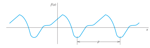
Fig. 258. Periodic function of period p
possibly at some points, and if there is some positive number p, called a period of, f(x) such that
![]()
(The function f(x) = tan x is a periodic function that is not defined for all real x but undefined for some points (more precisely, countably many points), that is x = ±π/2, ±π/2, ….)
The graph of a periodic function has the characteristic that it can be obtained by periodic repetition of its graph in any interval of length p (Fig. 258).
The smallest positive period is often called the fundamental period. (See Probs. 2–4.)
Familiar periodic functions are the cosine, sine, tangent, and cotangent. Examples of functions that are not periodic are x, x2, x3, ex, cosh x, and In x, to mention just a few.
If f(x) has period p, it also has the period 2p because (1) implies f(x + 2p) = f([x + p] + p) = f(x + p) = f(x), etc.; thus for any integer n = 1, 2, 3, …,
![]()
Furthermore if f(x) and g(x) have period p, then af(x) + bg(x) with any constants a and b also has the period p.
Our problem in the first few sections of this chapter will be the representation of various functions f(x) of period 2π in terms of the simple functions
![]()
All these functions have the period 2π. They form the so-called trigonometric system. Figure 259 shows the first few of them (except for the constant 1, which is periodic with any period).

Fig. 259. Cosine and sine functions having the period 2π (the first few members of the trigonometric system (3), except for the constant 1)
The series to be obtained will be a trigonometric series, that is, a series of the form
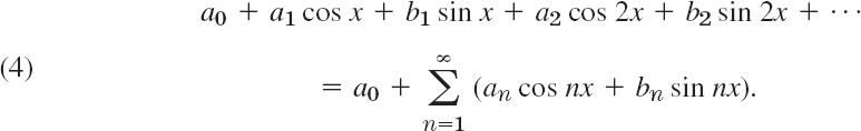
a0, a1, b1, a2, b2, … are constants, called the coefficients of the series. We see that each term has the period 2π. Hence if the coefficients are such that the series converges, its sum will be a function of period 2π.
Expressions such as (4) will occur frequently in Fourier analysis. To compare the expression on the right with that on the left, simply write the terms in the summation. Convergence of one side implies convergence of the other and the sums will be the same.
Now suppose that f(x) is a given function of period 2π and is such that it can be represented by a series (4), that is, (4) converges and, moreover, has the sum f(x). Then, using the equality sign, we write

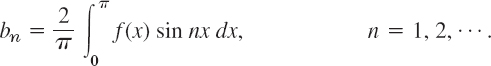
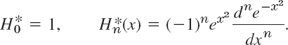
and call (5) the Fourier series of f(x). We shall prove that in this case the coefficients of (5) are the so-called Fourier coefficients of f(x), given by the Euler formulas
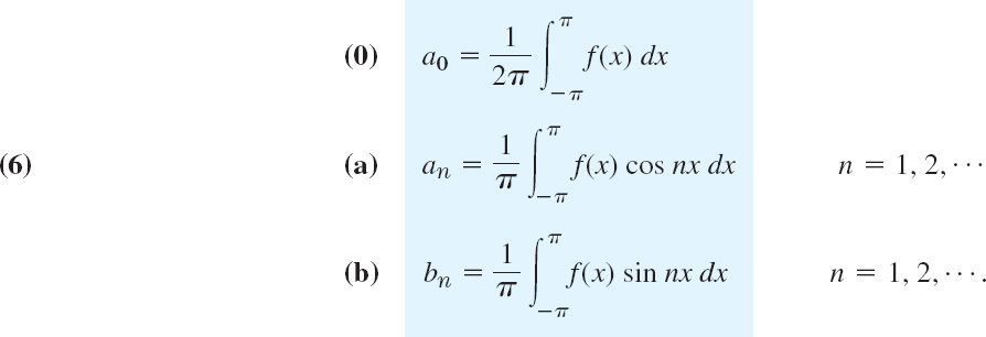
The name “Fourier series” is sometimes also used in the exceptional case that (5) with coefficients (6) does not converge or does not have the sum f(x)—this may happen but is merely of theoretical interest. (For Euler see footnote 4 in Sec. 2.5.)
A Basic Example
Before we derive the Euler formulas (6), let us consider how (5) and (6) are applied in this important basic example. Be fully alert, as the way we approach and solve this example will be the technique you will use for other functions. Note that the integration is a little bit different from what you are familiar with in calculus because of the n. Do not just routinely use your software but try to get a good understanding and make observations: How are continuous functions (cosines and sines) able to represent a given discontinuous function? How does the quality of the approximation increase if you take more and more terms of the series? Why are the approximating functions, called the partial sums of the series, in this example always zero at 0 and π? Why is the factor 1/n (obtained in the integration) important?
EXAMPLE 1 Periodic Rectangular Wave (Fig. 260)
Find the Fourier coefficients of the periodic function f(x) in Fig. 260. The formula is

Functions of this kind occur as external forces acting on mechanical systems, electromotive forces in electric circuits, etc. (The value of f(x) at a single point does not affect the integral; hence we can leave f(x) undefined at x = 0 and x = ±π.)
Solution. From (6.0) we obtain a0 = 0. This can also be seen without integration, since the area under the curve of f(x) between −π and π (taken with a minus sign where f(x) is negative) is zero. From (6a) we obtain the coefficients a1, a2, … of the cosine terms. Since f(x) is given by two expressions, the integrals from −π to π split into two integrals:

because sin nx = 0 at −π, 0, and π for all n = 1, 2, …. We see that all these cosine coefficients are zero. That is, the Fourier series of (7) has no cosine terms, just sine terms, it is a Fourier sine series with coefficients b1, b2, … obtained from (6b);
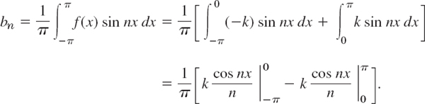
Since cos (−α) = cos α and cos 0 = 1, this yields
![]()
Now, cos π = −1, cos 2π = 1, cos 3π = −1 etc.; in general,

Hence the Fourier coefficients bn of our function are

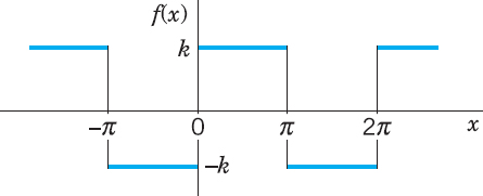
Fig. 260. Given function f(x) (Periodic reactangular wave)
Since the an are zero, the Fourier series f(x) of is
![]()
The partial sums are

Their graphs in Fig. 261 seem to indicate that the series is convergent and has the sum f(x), the given function. We notice that at x = 0 and x = π, the points of discontinuity of f(x), all partial sums have the value zero, the arithmetic mean of the limits −k and k of our function, at these points. This is typical.
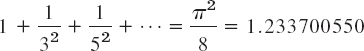
Furthermore, assuming that f(x) is the sum of the series and setting x = π/2, we have
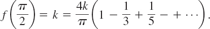
Thus

This is a famous result obtained by Leibniz in 1673 from geometric considerations. It illustrates that the values of various series with constant terms can be obtained by evaluating Fourier series at specific points.

Fig. 261. First three partial sums of the corresponding Fourier series
Derivation of the Euler Formulas (6)
The key to the Euler formulas (6) is the orthogonality of (3), a concept of basic importance, as follows. Here we generalize the concept of inner product (Sec. 9.3) to functions.
THEOREM 1 Orthogonality of the Trigonometric System (3)
The trigonometric system (3) is orthogonal on the interval −π ![]() x
x ![]() π (hence also on 0
π (hence also on 0 ![]() x
x ![]() 2π or any other interval of length 2π because of periodicity); that is, the integral of the product of any two functions in (3) over that interval is 0, so that for any integers n and m,
2π or any other interval of length 2π because of periodicity); that is, the integral of the product of any two functions in (3) over that interval is 0, so that for any integers n and m,

PROOF
This follows simply by transforming the integrands trigonometrically from products into sums. In (9a) and (9b), by (11) in App. A3.1,

Since m ≠ n (integer!), the integrals on the right are all 0. Similarly, in (9c), for all integer m and n (without exception; do you see why?)

Application of Theorem 1 to the Fourier Series (5)
We prove (6.0). Integrating on both sides of (5) from to −π to π, we get
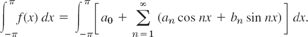
We now assume that termwise integration is allowed. (We shall say in the proof of Theorem 2 when this is true.) Then we obtain

The first term on the right equals 2πa0. Integration shows that all the other integrals are 0. Hence division by 2π gives (6.0).
We prove (6a). Multiplying (5) on both sides by cos mx with any fixed positive integer m and integrating from −π to π, we have

We now integrate term by term. Then on the right we obtain an integral of a0 cos mx which is 0; an integral of an cos nx cos mx, which is amπ for n = m and 0 for n ≠ m by (9a); and an integral of bn sin nx cos mx, which is 0 for all n and m by (9c). Hence the right side of (10) equals amπ. Division by π gives (6a) (with m instead of n).
We finally prove (6b). Multiplying (5) on both sides by sin mx with any fixed positive integer m and integrating from −π to π, we get

Integrating term by term, we obtain on the right an integral of a0 sin mx, which is 0; an integral of an cos nx sin mx, which is 0 by (9c); and an integral of bn sin nx sin mx, which is bmπ if n = m and 0 if n ≠ m, by (9b). This implies (6b) (with n denoted by m). This completes the proof of the Euler formulas (6) for the Fourier coefficients.
Convergence and Sum of a Fourier Series
The class of functions that can be represented by Fourier series is surprisingly large and general. Sufficient conditions valid in most applications are as follows.
THEOREM 2 Representation by a Fourier Series
Let f(x) be periodic with period 2π and piecewise continuous (see Sec. 6.1) in the interval −π ![]() x
x ![]() π. Furthermore, let f(x) have a left-hand derivative and a right-hand derivative at each point of that interval. Then the Fourier series (5) of f(x) [with coefficients (6)] converges. Its sum is f(x), except at points x0 where f(x) is discontinuous. There the sum of the series is the average of the left- and right-hand limits2 of f(x) at x0.
π. Furthermore, let f(x) have a left-hand derivative and a right-hand derivative at each point of that interval. Then the Fourier series (5) of f(x) [with coefficients (6)] converges. Its sum is f(x), except at points x0 where f(x) is discontinuous. There the sum of the series is the average of the left- and right-hand limits2 of f(x) at x0.
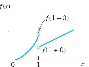
Fig. 262. Left- and right-hand limits  of the function
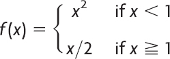
We prove convergence, but only for a continuous function f(x) having continuous first and second derivatives. And we do not prove that the sum of the series is f(x) because these proofs are much more advanced; see, for instance, Ref. [C12] listed in App. 1. Integrating (6a) by parts, we obtain

The first term on the right is zero. Another integration by parts gives

The first term on the right is zero because of the periodicity and continuity of f′(x). Since f″ is continuous in the interval of integration, we have
![]()
for an appropriate constant M. Furthermore, |cos nx| ![]() 1. It follows that
1. It follows that
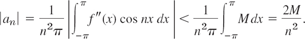
Similarly, |bn| < 2M/n2 for all n. Hence the absolute value of each term of the Fourier series of f(x) is at most equal to the corresponding term of the series

which is convergent. Hence that Fourier series converges and the proof is complete. (Readers already familiar with uniform convergence will see that, by the Weierstrass test in Sec. 15.5, under our present assumptions the Fourier series converges uniformly, and our derivation of (6) by integrating term by term is then justified by Theorem 3 of Sec. 15.5.)
EXAMPLE 2 Convergence at a Jump as Indicated in Theorem 2
The rectangular wave in Example 1 has a jump at x = 0. Its left-hand limit there is −k and its right-hand limit is k (Fig. 261). Hence the average of these limits is 0. The Fourier series (8) of the wave does indeed converge to this value when x = 0 because then all its terms are 0. Similarly for the other jumps. This is in agreement with Theorem 2.
Summary. A Fourier series of a given function f(x) of period 2π is a series of the form (5) with coefficients given by the Euler formulas (6). Theorem 2 gives conditions that are sufficient for this series to converge and at each x to have the value f(x), except at discontinuities of f(x), where the series equals the arithmetic mean of the left-hand and right-hand limits of f(x) at that point.
1–5 PERIOD, FUNDAMENTAL PERIOD
The fundamental period is the smallest positive period. Find it for
- cos x, sin x, cos 2x, sin 2x, cos πx, sin πx, cos 2πx, sin 2πx

- If f(x) and g(x) have period p, show that h(x) = af(x) + bg(x) (a, b, constant) has the period p. Thus all functions of period p from a vector space.
- Change of scale. If f(x) has period p, show that f(ax), a ≠ 0, and f(x/b), b ≠ 0, are periodic functions of x periods p/a and bp, repectively. Give examples.
- Show that f = const is periodic with any period but has no fundamental period.
6–10 GRAPHS OF 2π–PERIODIC FUNCTIONS
Sketch or graph f(x) which for −π < x < π is given as follows.
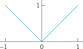
- 6. f(x) = |x|
- 7. f(x) = |sin x|, f(x) = sin |x|
- 8. f(x) = e−|x|, f(x) = |e−x|
- 9.

- 10.

- 11. Calculus review. Review integration techniques for integrals as they are likely to arise from the Euler formulas, for instance, definite integrals of x cos nx, x2 sin nx, e−2x cos nx, etc.
12–21 FOURIER SERIES
Find the Fourier series of the given function f(x), which is assumed to have the period 2π. Show the details of your work. Sketch or graph the partial sums up to that including cos 5x and sin 5x.
- 12. f(x) in Prob. 6
- 13. f(x) in Prob. 9
- 14. f(x) = x2 (−π < x < π)
- 15. f(x) = x2 (0 < x < 2π)
- 16.

- 17.

- 18.

- 19.
- 20.

- 21.

- 22. CAS EXPERIMENT. Graphing. Write a program for graphing partial sums of the following series. Guess from the graph what f(x) the series may represent. Confirm or disprove your guess by using the Euler formulas.

- 23. Discontinuities. Verify the last statement in Theorem 2 for the discontinuities of f(x) in Prob. 21.
- 24. CAS EXPERIMENT. Orthogonality. Integrate and graph the integral of the product cos mx cos nx (with various integer m and n of your choice) from −a to a as a function of a and conclude orthogonality of cos mx and cos nx (m ≠ n) for a = π from the graph. For what m and n will you get orthogonality for a = π/2, π/3, π/4? Other a? Extend the experiment to cos mx sin nx and sin mx sin nx.
- 25. CAS EXPERIMENT. Order of Fourier Coefficients. The order seems to be 1/n if f is discontinous, and 1/n2 if f is continuous but f′ = df/dx is discontinuous, 1/n3 if f and f′ are continuous but f″ is discontinuous, etc. Try to verify this for examples. Try to prove it by integrating the Euler formulas by parts. What is the practical significance of this?
11.2 Arbitrary Period. Even and Odd Functions. Half-Range Expansions
We now expand our initial basic discussion of Fourier series.
Orientation. This section concerns three topics:
- Transition from period 2π to any period 2L, for the function f, simply by a transformation of scale on the x-axis.
- Simplifications. Only cosine terms if f is even (“Fourier cosine series”). Only sine terms if f is odd (“Fourier sine series”).
- Expansion of f given for 0
 x L in two Fourier series, one having only cosine terms and the other only sine terms (“half-range expansions”).
1. From Period 2π to Any Period p = 2L
Clearly, periodic functions in applications may have any period, not just 2π as in the last section (chosen to have simple formulas). The notation p = 2L for the period is practical because L will be a length of a violin string in Sec. 12.2, of a rod in heat conduction in Sec. 12.5, and so on.
The transition from period 2π to be period p = 2L is effected by a suitable change of scale, as follows. Let f(x) have period p = 2L. Then we can introduce a new variable υ such that f(x), as a function of υ, has period 2π. If we set

then υ = ±π corresponds to x = ±L. This means that f, as a function of υ, has period 2π and, therefore, a Fourier series of the form

with coefficients obtained from (6) in the last section
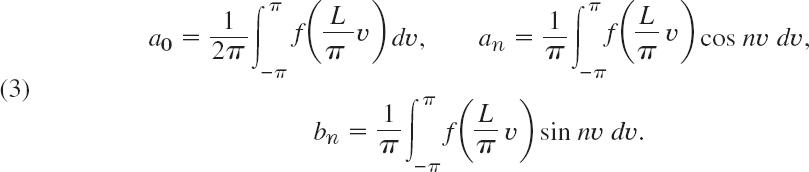
We could use these formulas directly, but the change to x simplifies calculations. Since
![]()
and we integrate over x from −L to L. Consequently, we obtain for a function f(x) of period 2L the Fourier series

with the Fourier coefficients of f(x) given by the Euler formulas (π/L in dx cancels 1/π in (3))

Just as in Sec. 11.1, we continue to call (5) with any coefficients a trigonometric series. And we can integrate from 0 to 2L or over any other interval of length p = 2L.
EXAMPLE 1 Periodic Rectangular Wave
Find the Fourier series of the function (Fig. 263)
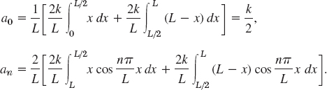
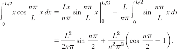
Solution. From (6.0) we obtain a0 = k/2 (verify!). From (6a) we obtain

Thus an = 0 if n is even and
![]()
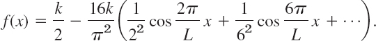
From (6b) we find that bn = 0 for n = 1, 2, …. Hence the Fourier series is a Fourier cosine series (that is, it has no sine terms)
![]()

Fig. 263. Example 1
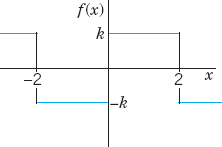
Fig. 264. Example 2
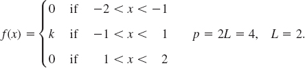
EXAMPLE 2 Periodic Rectangular Wave. Change of Scale
Find the Fourier series of the function (Fig. 264)

Solution. Since L = 2, we have in (3) υ = πx/2 and obtain from (8) in Sec. 11.1 with υ instead of x, that is,
![]()
the present Fourier series
![]()
Confirm this by using (6) and integrating.
A sinusoidal voltage E sin ωt, where t is time, is passed through a half-wave rectifier that clips the negative portion of the wave (Fig. 265). Find the Fourier series of the resulting periodic function

Solution. Since u = 0 when −L < t < 0, we obtain from (6.0), with t instead of x,
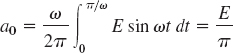
and from (6a), by using formula (11) in App. A3.1 with x = ωt and y = nωt,

If n = 1, the integral on the right is zero, and if n = 2, 3, …, we readily obtain
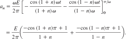
If n is odd, this is equal to zero, and for even n we have
![]()
In a similar fashion we find from (6b) that b1 = E/2 and bn = 0 for n = 2, 3, …. Consequently,
![]()

2. Simplifications: Even and Odd Functions
If f(x) is an even function, that is, f(−x) = f(x) (see Fig. 266), its Fourier series (5) reduces to a Fourier cosine series

with coefficients (note: integration from 0 to L only!)


If f(x) is an odd function, that is, f(−x) = −f(x) (see Fig. 267), its Fourier series (5) reduces to a Fourier sine series

with coefficients

These formulas follow from (5) and (6) by remembering from calculus that the definite integral gives the net area (= area above the axis minus area below the axis) under the curve of a function between the limits of integration. This implies

Formula (7b) implies the reduction to the cosine series (even f makes f(x) sin (nπx/L) odd since sin is odd) and to the sine series (odd f makes f(x) cos (nπx/L) odd since cos is even.) Similarly, (7a) reduces the integrals in (6*) and (6**) to integrals from 0 to L. These reductions are obvious from the graphs of an even and an odd function. (Give a formal proof.)
Even Function of Period 2π. If f is even and L = π, then
with coefficients

Odd Function of Period 2π. If f is odd and L = π, then

with coefficients
EXAMPLE 4 Fourier Cosine and Sine Series
The rectangular wave in Example 1 is even. Hence it follows without calculation that its Fourier series is a Fourier cosine series, the bn are all zero. Similarly, it follows that the Fourier series of the odd function in Example 2 is a Fourier sine series.
In Example 3 you can see that the Fourier cosine series represents ![]() . Can you prove that this is an even function?
. Can you prove that this is an even function?
Further simplifications result from the following property, whose very simple proof is left to the student.
THEOREM 1 Sum and Scalar Multiple
The Fourier coefficients of a sum f1 + f2 are the sums of the corresponding Fourier coefficients of f1 and f2.
The Fourier coefficients of cf are c times the corresponding Fourier coefficients of f.
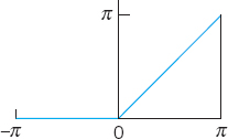
Find the Fourier series of the function (Fig. 268)
![]()

Fig. 268. The function f(x). Sawtooth wave

Fig. 269. Partial sums S1, S2, S3, S20 in Example 5
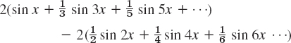
Solution. We have f = f1 + f2, where f1 = x and f2 = π. The Fourier coefficients of f2 are zero, except for the first one (the constant term), which is π. Hence, by Theorem 1, the Fourier coefficients an, bn are those of f1, except for a0, which is π. Since f1 is odd, an = 0 for n = 1, 2, …, and

Integrating by parts, we obtain

Hence ![]() , and the Fourier series of f(x) is
, and the Fourier series of f(x) is
![]()
3. Half-Range Expansions
Half-range expansions are Fourier series. The idea is simple and useful. Figure 270 explains it. We want to represent f(x) in Fig. 270. 0 by a Fourier series, where f(x) may be the shape of a distorted violin string or the temperature in a metal bar of length L, for example. (Corresponding problems will be discussed in Chap. 12.) Now comes the idea.
We could extend f(x) as a function of period L and develop the extended function into a Fourier series. But this series would, in general, contain both cosine and sine terms. We can do better and get simpler series. Indeed, for our given f we can calculate Fourier coefficients from (6*) or from (6**). And we have a choice and can take what seems more practical. If we use (6*), we get (5*). This is the even periodic extension f1 of f in Fig. 270a. If we choose (6**) instead, we get the (5**), odd periodic extension f2 of f in Fig. 270b.
Both extensions have period 2L. This motivates the name half-range expansions: f is given (and of physical interest) only on half the range, that is, on half the interval of periodicity of length 2L.
Let us illustrate these ideas with an example that we shall also need in Chap. 12.

Fig. 270. Even and odd extensions of period 2L
EXAMPLE 6 “Triangle” and Its Half-Range Expansions
Find the two half-range expansions of the function (Fig. 271)


Fig. 271. The given function in Example 6
Solution. (a) Even periodic extension. From (6*) we obtain
We consider an. For the first integral we obtain by integration by parts
Similarly, for the second integral we obtain

We insert these two results into the formula for an. The sine terms cancel and so does a factor L2. This gives

Thus,
![]()
and an = 0 if n ≠ 2, 6, 10, 14, …. Hence the first half-range expansion of f(x) is (Fig. 272a)
This Fourier cosine series represents the even periodic extension of the given function f(x), of period 2L.
(b) Odd periodic extension. Similarly, from (6**) we obtain
![]()
Hence the other half-range expansion of f(x) is (Fig. 272b)

The series represents the odd periodic extension of f(x), of period 2L.
Basic applications of these results will be shown in Secs. 12.3 and 12.5.

Fig. 272. Periodic extensions of f(x) in Example 6
PROBLEM SET 11.2
1–7 EVEN AND ODD FUNCTIONS
Are the following functions even or odd or neither even nor odd?
- ex, e−|x|, x3 cos nx, x2 tan πx, sinh x − cosh x
- sin2x, sin(x2), In x, x/(x2 + 1), x cot x
- Sums and products of even functions
- Sums and products of odd functions
- Absolute values of odd functions
- Product of an odd times an even function
- Find all functions that are both even and odd.
8–17 FOURIER SERIES FOR PERIOD p = 2L
Is the given function even or odd or neither even nor odd? Find its Fourier series. Show details of your work.
- 8.
- 9.
- 10.

- 11. f(x) = x2 (−1 < x < 1), p = 2
- 12. f(x) = 1 − x2/4 (−2 < x < 2), p = 4
- 13.

- 14.

- 15.

- 16. f(x) = x|x| (−1 < x < 1), p = 2
- 17.

- 18. Rectifier. Find the Fourier series of the function obtained by passing the voltage υ(t) = V0 cos 100πt through a half-wave rectifier that clips the negative half-waves.
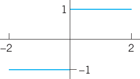
- 19. Trigonometric Identities. Show that the familiar identities
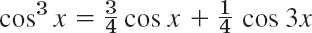 and
and 
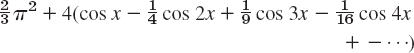
 can be interpreted as Fourier series expansions. Develop cos4x.
 - 20. Numeric Values. Using Prob. 11, show that

- 21. CAS PROJECT. Fourier Series of 2L-Periodic Functions. (a) Write a program for obtaining partial sums of a Fourier series (5). (b) Apply the program to Probs. 8–11, graphing the first few partial sums of each of the four series on common axes. Choose the first five or more partial sums until they approximate the given function reasonably well. Compare and comment.
- 22. Obtain the Fourier series in Prob. 8 from that in Prob. 17.
23–29 HALF-RANGE EXPANSIONS
Find (a) the Fourier cosine series, (b) the Fourier sine series. Sketch f(x) and its two periodic extensions. Show the details.
- 23.

- 24.

- 25.
- 26.

- 27.

- 28.
- 29. f(x) = sin x (0 < x < π)
- 30. Obtain the solution to Prob. 26 from that of Prob. 27.
11.3 Forced Oscillations
Fourier series have important applications for both ODEs and PDEs. In this section we shall focus on ODEs and cover similar applications for PDEs in Chap. 12. All these applications will show our indebtedness to Euler's and Fourier's ingenious idea of splitting up periodic functions into the simplest ones possible.
From Sec. 2.8 we know that forced oscillations of a body of mass m on a spring of modulus k are governed by the ODE

where y = y(t) is the displacement from rest, c the damping constant, k the spring constant (spring modulus), and r(t) the external force depending on time t. Figure 274 shows the model and Fig. 275 its electrical analog, an RLC- circuit governed by

We consider (1). If r(t) is a sine or cosine function and if there is damping (c > 0), then the steady-state solution is a harmonic oscillation with frequency equal to that of r(t). However, if r(t) is not a pure sine or cosine function but is any other periodic function, then the steady-state solution will be a superposition of harmonic oscillations with frequencies equal to that of r(t) and integer multiples of these frequencies. And if one of these frequencies is close to the (practical) resonant frequency of the vibrating system (see Sec. 2.8), then the corresponding oscillation may be the dominant part of the response of the system to the external force. This is what the use of Fourier series will show us. Of course, this is quite surprising to an observer unfamiliar with Fourier series, which are highly important in the study of vibrating systems and resonance. Let us discuss the entire situation in terms of a typical example.

Fig. 274. Vibrating system under consideration

Fig. 275. Electrical analog of the system in Fig. 274 (RLC-circuit)
EXAMPLE 1 Forced Oscillations under a Nonsinusoidal Periodic Driving Force
In (1), let m = 1 (g), c = 0.05 (g/sec), and k = 25 (g/sec2), so that (1) becomes
![]()
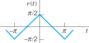
Fig. 276. Force in Example 1
where r(t) is measured in g · cm/sec2. Let (Fig. 276)

Find the steady-state solution y(t).
Solution. We represent r(t) by a Fourier series, finding

Then we consider the ODE

whose right side is a single term of the series (3). From Sec. 2.8 we know that the steady-state solution yn(t) of (4) is of the form
![]()
By substituting this into (4) we find that

Since the ODE (2) is linear, we may expect the steady-state solution to be
![]()
where yn is given by (5) and (6). In fact, this follows readily by substituting (7) into (2) and using the Fourier series of r(t), provided that termwise differentiation of (7) is permissible. (Readers already familiar with the notion of uniform convergence [Sec. 15.5] may prove that (7) may be differentiated term by term.)
From (6) we find that the amplitude of (5) is (a factor ![]() cancels out)
cancels out)

Values of the first few amplitudes are
![]()
Figure 277 shows the input (multiplied by 0.1) and the output. For n = 5 the quantity Dn is very small, the denominator of C5 is small, and C5 is so large that is the dominating term in (7). Hence the output is almost a harmonic oscillation of five times the frequency of the driving force, a little distorted due to the term y1, whose amplitude is about of that of y5. You could make the situation still more extreme by decreasing the damping constant c. Try it.
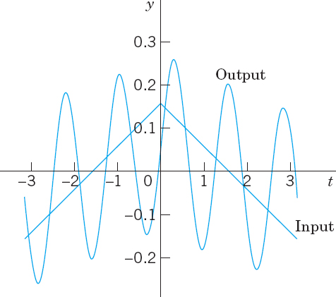
Fig. 277. Input and steady-state output in Example 1
PROBLEM SET 11.3
- Coefficients Cn. Derive the formula for Cn from An and Bn.
- Change of spring and damping. In Example 1, what happens to the amplitudes Cn if we take a stiffer spring, say, of k = 49? If we increase the damping?
- Phase shift. Explain the role of the Bn’s. What happens if we let c → 0?
- Differentiation of input. In Example 1, what happens if we replace r(t) with its derivative, the rectangular wave? What is the ratio of the new Cn to the old ones?
- Sign of coefficients. Some of the An in Example 1 are positive, some negative. All Bn are positive. Is this physically understandable?
6–11 GENERAL SOLUTION
Find a general solution of the ODE y″ + ω2y = r(t) with r(t) as given. Show the details of your work.
- 6. r(t) = sin αt + sin βt, ω2 ≠ α2, β2
- 7. r(t) = sin t, ω = 0.5, 0.9, 1.1, 1.5, 10
- 8. Rectifier. r(t) = π/4 |cos t| if − π < t < π and r(t + 2π) = r(t), |ω| ≠ 0, 2, 4, …
- 9. What kind of solution is excluded in Prob. 8 by |ω| ≠ 0, 2, 4, …?
- 10. Rectifier. r(t) = π/4 |sin t| if 0 < t < 2π and r(t + 2π) = r(t), |ω| ≠ 0, 2, 4, …
- 11.

- 12. CAS Program. Write a program for solving the ODE just considered and for jointly graphing input and output of an initial value problem involving that ODE. Apply the program to Probs. 7 and 11 with initial values of your choice.
13–16 STEADY-STATE DAMPED OSCILLATIONS
Find the steady-state oscillations of y″ + cy′ + y = r(t) with c > 0 and r(t) as given. Note that the spring constant is k = 1. Show the details. In Probs. 14–16 sketch r(t).
- 13.

- 14.

- 15. r(t) = t(π2 − t2) if −π < t < π and r(t + 2π) = r(t)
- 16.

17–19 RLC-CIRCUIT
Find the steady-state current I(t) in the RLC-circuit in Fig. 275, where R = 10Ω, L = 1 H, C = 10−1 F and with E(t) V as follows and periodic with period 2π. Graph or sketch the first four partial sums. Note that the coefficients of the solution decrease rapidly. Hint. Remember that the ODE contains E′(t), not E(t), cf. Sec. 2.9.
- 17.

- 18.

- 19.

- 20. CAS EXPERIMENT. Maximum Output Term. Graph and discuss outputs of y″ + cy′ + ky = r(t) with r(t) as in Example 1 for various c and k with emphasis on the maximum Cn and its ratio to the second largest |Cn|.
11.4 Approximation by Trigonometric Polynomials
Fourier series play a prominent role not only in differential equations but also in approximation theory, an area that is concerned with approximating functions by other functions—usually simpler functions. Here is how Fourier series come into the picture.
Let f(x) be a function on the interval −π ![]() x
x ![]() π that can be represented on this interval by a Fourier series. Then the Nth partial sum of the Fourier series
π that can be represented on this interval by a Fourier series. Then the Nth partial sum of the Fourier series

is an approximation of the given f(x). In (1) we choose an arbitrary N and keep it fixed. Then we ask whether (1) is the “best” approximation of f by a trigonometric polynomial of the same degree N, that is, by a function of the form

Here, “best” means that the “error” of the approximation is as small as possible.
Of course we must first define what we mean by the error of such an approximation. We could choose the maximum of |f(x) − F(x)|. But in connection with Fourier series it is better to choose a definition of error that measures the goodness of agreement between f and F on the whole interval −π ![]() x
x ![]() π. This is preferable since the sum f of a Fourier series may have jumps: F in Fig. 278 is a good overall approximation of f, but the maximum of |f(x) − F(x)| (more precisely, the supremum) is large. We choose
π. This is preferable since the sum f of a Fourier series may have jumps: F in Fig. 278 is a good overall approximation of f, but the maximum of |f(x) − F(x)| (more precisely, the supremum) is large. We choose
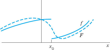
Fig. 278. Error of approximation
This is called the square error of F relative to the function f on the interval −π ![]() x
x ![]() π. Clearly, E
π. Clearly, E ![]() 0.
0.
N being fixed, we want to determine the coefficients in (2) such that E is minimum. Since (f − F)2 = f2 − 2fF + F2, we have

We square (2), insert it into the last integral in (4), and evaluate the occurring integrals. This gives integrals of cos2 nx and sin2 nx(n ![]() 1), which equal π, and integrals of cos nx, sin nx, and (cos nx)(sin mx), which are zero (just as in Sec. 11.1). Thus
1), which equal π, and integrals of cos nx, sin nx, and (cos nx)(sin mx), which are zero (just as in Sec. 11.1). Thus

We now insert (2) into the integral of f F in (4). This gives integrals of f cos nx as well as f sin nx, just as in Euler's formulas, Sec. 11.1, for an and bn (each multiplied by An or Bn).
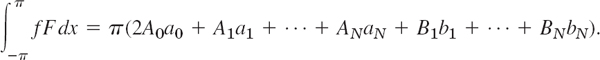
With these expressions, (4) becomes
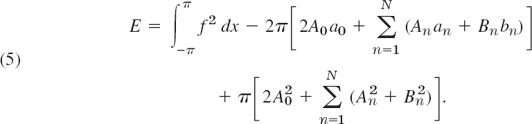
We now take An = an and Bn = bn in (2). Then in (5) the second line cancels half of the integral-free expression in the first line. Hence for this choice of the coefficients of F the square error, call it E*, is

We finally subtract (6) from (5). Then the integrals drop out and we get terms ![]() and similar terms (Bn − bn)2:
and similar terms (Bn − bn)2:

Since the sum of squares of real numbers on the right cannot be negative,
![]()
and E = E* if and only if A0 = a0, …, BN = bN. This proves the following fundamental minimum property of the partial sums of Fourier series.
THEOREM 1 Minimum Square Error
The square error of F in (2) (with fixed N) relative to f on the interval −π ![]() x
x ![]() π is minimum if and only if the coefficients of F in (2) are the Fourier coefficients of f. This minimum value E* is given by (6).
π is minimum if and only if the coefficients of F in (2) are the Fourier coefficients of f. This minimum value E* is given by (6).
From (6) we see that E* cannot increase as N increases, but may decrease. Hence with increasing N the partial sums of the Fourier series of f yield better and better approximations to f, considered from the viewpoint of the square error.
Since E* ![]() 0 and (6) holds for every N, we obtain from (6) the important Bessel's inequality
0 and (6) holds for every N, we obtain from (6) the important Bessel's inequality

for the Fourier coefficients of any function f for which integral on the right exists. (For F. W. Bessel see Sec. 5.5.)
It can be shown (see [C12] in App. 1) that for such a function f, Parseval's theorem holds; that is, formula (7) holds with the equality sign, so that it becomes Parseval's identity3

EXAMPLE 1 Minimum Square Error for the Sawtooth Wave
Compute the minimum square error E* of F(x) with N = 1, 2, …, 10, 20, …, and 1000 relative to
![]()
on the interval −π ![]() x
x ![]() π.
π.
Solution.  by Example 3 in Sec. 11.3. From this and (6),

Numeric values are:
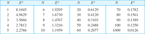

Fig. 279. F with N = 20 in Example 1
F = S1, S2, S3 are shown in Fig. 269 in Sec. 11.2, and F = S20 is shown in Fig. 279. Although |f(x) − F(x)| is large at ±π (how large?), where f is discontinuous, F approximates f quite well on the whole interval, except near ±π, where “waves” remain owing to the “Gibbs phenomenon,” which we shall discuss in the next section.
Can you think of functions f for which E* decreases more quickly with increasing N?
PROBLEM SET 11.4
- CAS Problem. Do the numeric and graphic work in Example 1 in the text.
2–5 MINIMUM SQUARE ERROR
Find the trigonometric polynomial F(x) of the form (2) for which the square error with respect to the given f(x) on the interval −π < x < π is minimum. Compute the minimum value for N = 1, 2, …, 5 (or also for larger values if you have a CAS).
- 2. f(x) = x (−π < x < π)
- 3. f(x) = |x| (−π < x < π)
- 4. f(x) = x2 (−π < x < π)
- 5.

- 6. Why are the square errors in Prob. 5 substantially larger than in Prob. 3?
- 7. f(x) = x3 (−π < x < π)
- 8. f(x) = |sin x| (−π < x < π), full-wave rectifier
- 9. Monotonicity. Show that the minimum square error (6) is a monotone decreasing function of N. How can you use this in practice?
- 10. CAS EXPERIMENT. Size and Decrease of E *. Compare the size of the minimum square error for functions of your choice. Find experimentally the factors on which the decrease of E* with N depends. For each function considered find the smallest N such that E* < 0.1.
11–15 PARSEVALS'S IDENTITY
Using (8), prove that the series has the indicated sum. Compute the first few partial sums to see that the convergence is rapid.


11.5 Sturm–Liouville Problems. Orthogonal Functions
The idea of the Fourier series was to represent general periodic functions in terms of cosines and sines. The latter formed a trigonometric system. This trigonometric system has the desirable property of orthogonality which allows us to compute the coefficient of the Fourier series by the Euler formulas.
The question then arises, can this approach be generalized? That is, can we replace the trigonometric system of Sec. 11.1 by other orthogonal systems (sets of other orthogonal functions)? The answer is “yes” and will lead to generalized Fourier series, including the Fourier–Legendre series and the Fourier–Bessel series in Sec. 11.6.
To prepare for this generalization, we first have to introduce the concept of a Sturm–Liouville Problem. (The motivation for this approach will become clear as you read on.) Consider a second-order ODE of the form

on some interval a ![]() x
x ![]() b, satisfying conditions of the form
b, satisfying conditions of the form

Here λ is a parameter, and k1, k2, l1, l2 are given real constants. Furthermore, at least one of each constant in each condition (2) must be different from zero. (We will see in Example 1 that, if p(x) = r(x) = 1 and q(x) = 0, then sin ![]() and cos
and cos ![]() satisfy (1) and constants can be found to satisfy (2).) Equation (1) is known as a Sturm–Liouville equation.4 Together with conditions 2(a), 2(b) it is know as the Sturm–Liouville problem. It is an example of a boundary value problem.
satisfy (1) and constants can be found to satisfy (2).) Equation (1) is known as a Sturm–Liouville equation.4 Together with conditions 2(a), 2(b) it is know as the Sturm–Liouville problem. It is an example of a boundary value problem.
A boundary value problem consists of an ODE and given boundary conditions referring to the two boundary points (endpoints) x = a and x = b of a given interval a ![]() x
x ![]() b.
b.
The goal is to solve these type of problems. To do so, we have to consider
Eigenvalues, Eigenfunctions
Clearly, y ≡ 0 is a solution—the “trivial solution”—of the problem (1), (2) for any λ because (1) is homogeneous and (2) has zeros on the right. This is of no interest. We want to find eigenfunctions y(x), that is, solutions of (1) satisfying (2) without being identically zero. We call a number λ for which an eigenfunction exists an eigenvalue of the Sturm–Liouville problem (1), (2).
Many important ODEs in engineering can be written as Sturm–Liouville equations. The following example serves as a case in point.
EXAMPLE 1 Trigonometric Functions as Eigenfunctions. Vibrating String
Find the eigenvalues and eigenfunctions of the Sturm–Liouville problem
![]()
This problem arises, for instance, if an elastic string (a violin string, for example) is stretched a little and fixed at its ends x = 0 and x = π and then allowed to vibrate. Then y(x) is the “space function” of the deflection u(x, t) of the string, assumed in the form u(x, t) = y(x)w(t), where t is time. (This model will be discussed in great detail in Secs, 12.2–12.4.)
Solution. From (1) nad (2) we see that p = 1, q = 0, r = 1 in (1), and a = 0, b = π, k1 = l1 = 1, k2 = l2 = 0 in (2). For negative λ = −v2 a general solution of the ODE in (3) is y(x) = c1evx + c2e−vx. From the boundary conditions we obtain c1 = c2 = 0, so that y ≡ 0, which is not an eigenfunction. For λ = 0 the situation is similar. For positive λ = v2 a general solution is
![]()
From the first boundary condition we obtain y(0) = A = 0. The second boundary condition then yields
![]()
For ν = 0 we have y ≡ 0. For λ = ν2 = 1, 4, 9, 16, …, taking B = 1, we obtain
![]()
Hence the eigenvalues of the problem are λ = v2, where v = 1, 2, …, and corresponding eigenfunctions are y(x) = sin vx, where v = 1, 2 ….
Note that the solution to this problem is precisely the trigonometric system of the Fourier series considered earlier. It can be shown that, under rather general conditions on the functions p, q, r in (1), the Sturm–Liouville problem (1), (2) has infinitely many eigenvalues. The corresponding rather complicated theory can be found in Ref. [All] listed in App. 1.
Furthermore, if p, q, r, and p′ in (1) are real-valued and continuous on the interval a ![]() x
x ![]() b and r is positive throughout that interval (or negative throughout that interval), then all the eigenvalues of the Sturm–Liouville problem (1), (2) are real. (Proof in App. 4.) This is what the engineer would expect since eigenvalues are often related to frequencies, energies, or other physical quantities that must be real.
b and r is positive throughout that interval (or negative throughout that interval), then all the eigenvalues of the Sturm–Liouville problem (1), (2) are real. (Proof in App. 4.) This is what the engineer would expect since eigenvalues are often related to frequencies, energies, or other physical quantities that must be real.
The most remarkable and important property of eigenfunctions of Sturm–Liouville problems is their orthogonality, which will be crucial in series developments in terms of eigenfunctions, as we shall see in the next section. This suggests that we should next consider orthogonal functions.
Orthogonal Functions
Functions y1(x), y2(x), … defined on some interval a ![]() x
x ![]() b are called orthogonal on this interval with respect to the weight function r(x) > 0 if for all m and all n different from m,
b are called orthogonal on this interval with respect to the weight function r(x) > 0 if for all m and all n different from m,
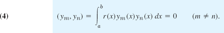
(ym, yn) is a standard notation for this integral. The norm ||ym|| of ym is defined by
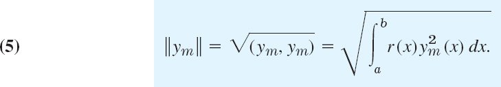
Note that this is the square root of the integral in (4) with n = m.
The functions y1, y2, … are called orthonormal on a ![]() x
x ![]() b if they are orthogonal on this interval and all have norm 1. Then we can write (4), (5) jointly by using the Kronecker symbol5 δmn, namely,
b if they are orthogonal on this interval and all have norm 1. Then we can write (4), (5) jointly by using the Kronecker symbol5 δmn, namely,

If r(x) = 1, we more briefly call the functions orthogonal instead of orthogonal with respect to r(x) = 1; similarly for orthognormality. Then

The next example serves as an illustration of the material on orthogonal functions just discussed.
EXAMPLE 2 Orthogonal Functions. Orthonormal Functions. Notation
The functions ym(x) = sin mx, m = 1, 2, … form an orthogonal set on the interval −π ![]() x
x ![]() π, because for m ≠ n we obtain by integration [see (11) in App. A3.1]
π, because for m ≠ n we obtain by integration [see (11) in App. A3.1]

The norm ![]() equals
equals ![]() because
because

Hence the corresponding orthonormal set, obtained by division by the norm, is

Theorem 1 shows that for any Sturm–Liouville problem, the eigenfunctions associated with these problems are orthogonal. This means, in practice, if we can formulate a problem as a Sturm–Liouville problem, then by this theorem we are guaranteed orthogonality.
THEOREM 1 Orthogonality of Eigenfunctions of Sturm–Liouville Problems
Suppose that the functions p, q, r, and p′ in the Sturm–Liouville equation (1) are real-valued and continuous and r(x) > 0 on the interval a ![]() x
x ![]() b. Let ym(x) and yn(x) be eigenfunctions of the Sturm–Liouville problem (1), (2) that correspond to different eigenvalues λm and λn, respectively. Then ym, yn are orthogonal on that interval with respect to the weight function r, that is,
b. Let ym(x) and yn(x) be eigenfunctions of the Sturm–Liouville problem (1), (2) that correspond to different eigenvalues λm and λn, respectively. Then ym, yn are orthogonal on that interval with respect to the weight function r, that is,

If p(a) = 0, then (2a) can be dropped from the problem. If p(b) = 0, then (2b) can be dropped. [It is then required that y and y′ remain bounded at such a point, and the problem is called singular, as opposed to a regular problem in which (2) is used.]
If p(a) = p(b), then (2) can be replaced by the “periodic boundary conditions”
![]()
The boundary value problem consisting of the Sturm–Liouville equation (1) and the periodic boundary conditions (7) is called a periodic Sturm–Liouville problem.
By assumption, ym and yn satisfy the Sturm–Liouville equations
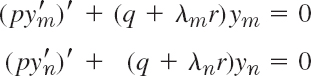
respectively. We multiply the first equation by yn, the second by −ym, and add,
![]()
where the last equality can be readily verified by performing the indicated differentiation of the last expression in brackets. This expression is continuous on a ![]() x
x ![]() b since p and p′ are continuous by assumption and ym, yn are solutions of (1). Integrating over x from a to b, we thus obtain
b since p and p′ are continuous by assumption and ym, yn are solutions of (1). Integrating over x from a to b, we thus obtain

The expression on the right equals the sum of the subsequent Lines 1 and 2,

Hence if (9) is zero, (8) with λm − λn ≠ 0 implies the orthogonality (6). Accordingly, we have to show that (9) is zero, using the boundary conditions (2) as needed.
Case 1. p(a) = p(b) = 0. Clearly, (9) is zero, and (2) is not needed.
Case 2. p(a) ≠ 0, p(b) = 0. Line 1 of (9) is zero. Consider Line 2. From (2a) we have

Let k2 ≠ 0. We multiply the first equation by ym(a), the last by −yn(a) and add,
![]()
This is k2 times Line 2 of (9), which thus is zero since k2 ≠ 0. If k2 = 0, then k1 ≠ 0 by assumption, and the argument of proof is similar.
Case 3. p(a) = 0, p(b) ≠ 0. Line 2 of (9) is zero. From (2b) it follows that Line 1 of (9) is zero; this is similar to Case 2.
Case 4. p(a) ≠ 0, p(b) ≠ 0. We use both (2a) and (2b) and proceed as in Cases 2 and 3.
Case 5. p(a) = p(b). Then (9) becomes
![]()
The expression in brackets […] is zero, either by (2) used as before, or more directly by (7). Hence in this case, (7) can be used instead of (2), as claimed. This completes the proof of Theorem 1.
EXAMPLE 3 Application of Theorem 1. Vibrating String
The ODE in Example 1 is a Sturm–Liouville equation with p = 1, q = 0 and r = 1. From Theorem 1 it follows that the eigenfunctions ym = sin mx (m = 1, 2, …) are orthogonal on the interval 0 ![]() x
x ![]() π.
π.
Example 3 confirms, from this new perspective, that the trigonometric system underlying the Fourier series is orthogonal, as we knew from Sec. 11.1.
EXAMPLE 4 Application of Theorem 1. Orthogonlity of the Legendre Polynomials
Legendre's equation (1 − x2)y″ − 2xy′ + n(n + 1)y = 0 may be written
![]()
Hence, this is a Sturm–Liouville equation (1) with p = 1 − x2, q = 0, and r = 1. Since p(−1) = p(1) = 0, we need no boundary conditions, but have a “singular” Sturm–Liouville problem on the interval −1 ![]() x
x ![]() 1. We know that for n = 0, 1, …, hence λ = 0, 1·2, 2·3, …, the Legendre polynomials Pn(x) are solutions of the problem. Hence these are the eigenfunctions. From Theorem 1 it follows that they are orthogonal on that interval, that is,
1. We know that for n = 0, 1, …, hence λ = 0, 1·2, 2·3, …, the Legendre polynomials Pn(x) are solutions of the problem. Hence these are the eigenfunctions. From Theorem 1 it follows that they are orthogonal on that interval, that is,

What we have seen is that the trigonometric system, underlying the Fourier series, is a solution to a Sturm–Liouville problem, as shown in Example 1, and that this trigonometric system is orthogonal, which we knew from Sec. 11.1 and confirmed in Example 3.
PROBLEM SET 11.5
- Proof of Theorem 1. Carry out the details in Cases 3 and 4.
2–6 ORTHOGONALITY
- 2. Normalization of eigenfunctions ym of (1), (2) means that we multiply ym by a nonzero constant cm such that cmym has norm 1. Show that Zm = cym with any c ≠ 0 is an eigenfunction for the eigenvalue corresponding to ym.
- 3. Change of x. Show that if the functions y0(x), y1(x), … form an orthogonal set on an interval a x b (with r(x) = 1), then the functions y0(ct + k), y1(ct + k)…, c > 0, form an orthogonal set on the interval (a − k)/c t (b − k)/c.
- 4. Change of x. Using Prob. 3, derive the orthogonality of 1, cos πx, sin πx, cos 2πx, sin 2πx, … on −1 x 1 (r(x) = 1) from that of 1, cos x, sin x, cos 2x, sin 2x, … on −π x π.
- 5. Legendre polynomials. Show that the functions Pn(cos θ), n = 0, 1, …, from an orthogonal set on the interval 0 θ π with respect to the weight function sin θ.
- 6. Tranformation to Sturm–Liouville form. Show that y″ + fy′ + (g + λh)y = 0 takes the form (1) if you set p = exp (∫fdx), q = pg, r = hp. Why would you do such a transformation?
7–15 STURM–LIOUVILLE PROBLEMS
Find the eigenvalues and eigenfunctions. Verify orthogonality. Start by writing the ODE in the form (1), using Prob. 6. Show details of your work.
- 7. y″ + λy = 0, y(0) = 0, y(10) = 0
- 8. y″ + λy = 0, y(0) = 0, y(L) = 0
- 9. y″ + λy = 0, y(0) = 0, y′(L) = 0
- 10. y″ + λy = 0, y(0) = y(1), y′(0) = y′(1)
- 11. (y′/x)′ + (λ + 1)y/x3 = 0, y(1) = 0, y(eπ) = 0. (Set x = et.)
- 12. y″ − 2y′ + (λ + 1)y = 0, y(0) = 0, y(1) = 0
- 13. y″ − 8y′ + (λ + 16)y = 0, y(0) = 0, y(π) = 0
- 14. TEAM PROJECT. Special Functions. Orthogonal polynomials play a great role in applications. For this reason, Legendre polynomials and various other orthogonal polynomials have been studied extensively; see Refs. [GenRef1], [GenRef10] in App. 1. Consider some of the most important ones as follows.
(a) Chebyshev polynomials6 of the first and second kind are defined by

respectively, where n = 0, 1, …. Show that

Show that the Chebyshev polynomials Tn(x) are orthogonal on the interval −1
x 1 with respect to the weight function  . (Hint. To evaluate the integral, set arccos x = θ.) Verify that Tn(x), n = 0, 1, 2, 3, satisfy the Chebyshev equation
(b) Orthogonality on an infinite interval: Laguerre polynomials7 are defined by L0 = 1, and

Show that

Prove that the Laguerre polynomials are orthogonal on the positive axis 0
x < ∞ with respect to the weight function r(x) = e−x. Hint. Since the highest power in Lm is xm, it suffices to show that for ∫e−xxkLndx = 0 for k < n. Do this by k integrations by parts.
11.6 Orthogonal Series. Generalized Fourier Series
Fourier series are made up of the trigonometric system (Sec. 11.1), which is orthogonal, and orthogonality was essential in obtaining the Euler formulas for the Fourier coefficients. Orthogonality will also give us coefficient formulas for the desired generalized Fourier series, including the Fourier–Legendre series and the Fourier–Bessel series. This generalization is as follows.
Let y0, y1, y2, … be orthogonal with respect to a weight function r(x) on an interval a ![]() x
x ![]() b, and let f(x) be a function that can be represented by a convergent series
b, and let f(x) be a function that can be represented by a convergent series
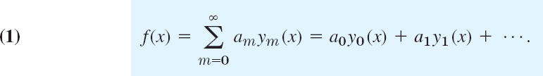
This is called an orthogonal series, orthogonal expansion, or generalized Fourier series. If the ym are the eigenfunctions of a Sturm–Liouville problem, we call (1) an eigenfunction expansion. In (1) we use again m for summation since n will be used as a fixed order of Bessel functions.
Given f(x), we have to determine the coefficients in (1), called the Fourier constants of f(x) with respect to y0, y1…. Because of the orthogonality, this is simple. Similarly to Sec. 11.1, we multiply both sides of (1) by r(x)yn(x) (n fixed) and then integrate on
both sides from a to b. We assume that term-by-term integration is permissible. (This is justified, for instance, in the case of “uniform convergence,” as is shown in Sec. 15.5.) Then we obtain

Because of the orthogonality all the integrals on the right are zero, except when m = n. Hence the whole infinite series reduces to the single term
![]()
Assuming that all the functions yn have nonzero norm, we can divide by ||yn||2; writing again m for n, to be in agreement with (1), we get the desired formula for the Fourier constants
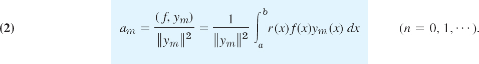
This formula generalizes the Euler formulas (6) in Sec. 11.1 as well as the principle of their derivation, namely, by orthogonality.
EXAMPLE 1 Fourier–Legendre Series
A Fourier–Legendre series is an eigenfunction expansion

in terms of Legendre polynomials (Sec. 5.3). The latter are the eigenfunctions of the Sturm–Liouville problem in Example 4 of Sec. 11.5 on the interval −1 ![]() x
x ![]() 1. We have r(x) = 1 for Legendre's equation, and (2) gives
1. We have r(x) = 1 for Legendre's equation, and (2) gives

because the norm is

as we state without proof. The proof of (4) is tricky; it uses Rodrigues's formula in Problem Set 5.2 and a reduction of the resulting integral to a quotient of gamma functions.
For instance, let f(x) = sin πx. Then we obtain the coefficients

Hence the Fourier–Legendre series of sin πx is
![]()
The coefficient of P13 is about 3 · 10−7. The sum of the first three nonzero terms gives a curve that practically coincides with the sine curve. Can you see why the even-numbered coefficients are zero? Why a3 is the absolutely biggest coefficient?
EXAMPLE 2 Fourier–Bessel Series
These series model vibrating membranes (Sec. 12.9) and other physical systems of circular symmetry. We derive these series in three steps.
Step 1. Bessel's equation as a Sturm–Liouville equation. The Bessel function Jn(x) with fixed integer n ![]() 0 satisfies Bessel's equation (Sec. 5.5)
0 satisfies Bessel's equation (Sec. 5.5)
![]()
where ![]() and
and ![]() . We set
. We set ![]() . Then
. Then ![]() and by the chain rule,
and by the chain rule, ![]()
![]() . In the first two terms of Bessel's equation, k2 and k drop out and we obtain
. In the first two terms of Bessel's equation, k2 and k drop out and we obtain
![]()
Dividing by x and using ![]() gives the Sturm–Liouville equation
gives the Sturm–Liouville equation

with p(x) = x, q(x) = −n2/x, r(x) = x and parameter λ = k2. Since p(0) = 0, Theorem 1 in Sec. 11.5 implies orthogonality on an interval 0 ![]() x
x ![]() R (R given, fixed) of those solutions Jn(kx) that are zero at x = R, that is,
R (R given, fixed) of those solutions Jn(kx) that are zero at x = R, that is,
![]()
Note that q(x) = −n2/x is discontinuous at 0, but this does not affect the proof of Theorem 1.
Step 2. Orthogonality. It can be shown (see Ref. [A13]) that ![]() has infinitely many zeros, say,
has infinitely many zeros, say, ![]() (see Fig. 110 in Sec. 5.4 for n = 0 and 1). Hence we must have
(see Fig. 110 in Sec. 5.4 for n = 0 and 1). Hence we must have
![]()
This proves the following orthogonality property.
THEOREM 1 Orthogonality of Bessel Functions
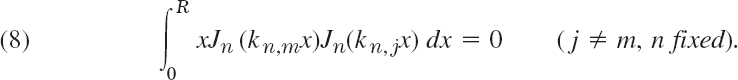
For each fixed nonnegative integer n the sequence of Bessel functions of the first kind Jn(kn, 1x), Jn(kn, 2x), … with kn,m as in (7) forms an orthogonal set on the interval 0 ![]() x
x ![]() R with respect to the weight function r(x) = x that is,
R with respect to the weight function r(x) = x that is,
Hence we have obtained infinitely many orthogonal sets of Bessel functions, one for each of J0, J1, J2, …. Each set is orthogonal on an interval 0 ![]() x
x ![]() R with a fixed positive R of our choice and with respect to the weight x. The orthogonal set for Jn is Jn(kn,1x), Jn(kn,2x), Jn(kn,3x), …, where n is fixed and kn,m is given by (7).
R with a fixed positive R of our choice and with respect to the weight x. The orthogonal set for Jn is Jn(kn,1x), Jn(kn,2x), Jn(kn,3x), …, where n is fixed and kn,m is given by (7).
Step 3. Fourier–Bessel series. The Fourier–Bessel series corresponding to Jn (n fixed) is

The coefficients are (with αn,m = kn,mR)

because the square of the norm is

as we state without proof (which is tricky; see the discussion beginning on p. 576 of [A13]).
EXAMPLE 3 Special Fourier–Bessel Series
For instance, let us consider f(x) = 1 − x2 and take R = 1 and n = 0 in the series (9), simply writing λ for α0,m. Then kn,m = α0,m = λ = 2.405, 5.520, 8.654, 11.792, etc. (use a CAS or Table A1 in App. 5). Next we calculate the coefficients am by (10)

This can be integrated by a CAS or by formulas as follows. First use [xJ1(λx)]′ = λxJ0(λx) from Theorem 1 in Sec. 5.4 and then integration by parts,
![]()
The integral-free part is zero. The remaining integral can be evaluated by [x2J2(λx)]′ = λx2J1(λx) from Theorem 1 in Sec. 5.4. This gives
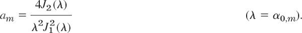
Numeric values can be obtained from a CAS (or from the table on p. 409 of Ref. [GenRef1] in App. 1, together with the formula J2 = 2x−1J1 − J0 in Theorem 1 of Sec. 5.4). This gives the eigenfunction expansion of 1 − x2 in terms of Bessel functions J0, that is,
![]()
A graph would show that the curve of and that of 1 − x2 the sum of first three terms practically coincide.
Mean Square Convergence. Completeness
Ideas on approximation in the last section generalize from Fourier series to orthogonal series (1) that are made up of an orthonormal set that is “complete,” that is, consists of “sufficiently many” functions so that (1) can represent large classes of other functions (definition below).
In this connection, convergence is convergence in the norm, also called mean-square convergence; that is, a sequence of functions fk is called convergent with the limit f if
![]()
written out by (5) in Sec. 11.5 (where we can drop the square root, as this does not affect the limit)

Accordingly, the series (1) converges and represents f if

where sk is the kth partial sum of (1).

Note that the integral in (13) generalizes (3) in Sec. 11.4.
We now define completeness. An orthonormal set y0, y1, … on an interval a ![]() x
x ![]() b is complete in a set of functions S defined on a
b is complete in a set of functions S defined on a ![]() x
x ![]() b if we can approximate every f belonging to S arbitrarily closely in the norm by a linear combination a0y0 + a1y1 + … + akyk, that is, technically, if for every ε > 0 we can find constants a0, …,ak (with k large enough) such that
b if we can approximate every f belonging to S arbitrarily closely in the norm by a linear combination a0y0 + a1y1 + … + akyk, that is, technically, if for every ε > 0 we can find constants a0, …,ak (with k large enough) such that
![]()
Ref. [GenRef7] in App. 1 uses the more modern term total for complete.
We can now extend the ideas in Sec. 11.4 that guided us from (3) in Sec. 11.4 to Bessel's and Parseval's formulas (7) and (8) in that section. Performing the square in (13) and using (14), we first have (analog of (4) in Sec. 11.4)

The first integral on the right equals ![]() because ∫rymyl dx = 0 for m ≠ 1, and
because ∫rymyl dx = 0 for m ≠ 1, and ![]() . In the second sum on the right, the integral equals am, by (2) with ||ym||2 = 1. Hence the first term on the right cancels half of the second term, so that the right side reduces to (analog of (6) in Sec. 11.4)
. In the second sum on the right, the integral equals am, by (2) with ||ym||2 = 1. Hence the first term on the right cancels half of the second term, so that the right side reduces to (analog of (6) in Sec. 11.4)

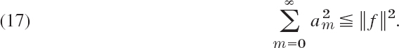
This is nonnegative because in the previous formula the integrand on the left is nonnegative (recall that the weight r(x) is positive!) and so is the integral on the left. This proves the important Bessel's inequality (analog of (7) in Sec. 11.4)

Here we can let k → ∞, because the left sides form a monotone increasing sequence that is bounded by the right side, so that we have convergence by the familiar Theorem 1 in App. A.3.3 Hence
Furthermore, if y0, y1, … is complete in a set of functions S, then (13) holds for every f belonging to S. By (13) this implies equality in (16) with k → ∞. Hence in the case of completeness every f in S saisfies the so-called Parseval equality (analog of (8) in Sec. 11.4)

As a consequence of (18) we prove that in the case of completeness there is no function orthogonal to every function of the orthonormal set, with the trivial exception of a function of zero norm:
Let y0, y1, … be a complete orthonormal set on a ![]() x
x ![]() b in a set of functions S. Then if a function f belongs to S and is orthogonal to every ym, it must have norm zero. In particular, if f is continuous, then f must be identically zero.
b in a set of functions S. Then if a function f belongs to S and is orthogonal to every ym, it must have norm zero. In particular, if f is continuous, then f must be identically zero.
PROOF
Since f is orthogonal to every ym the left side of (18) must be zero. If f is continuous, then ||f|| = 0 implies f(x) ≡ 0, as can be seen directly from (5) in Sec. 11.5 with f instead of ym because r(x) > 0 by assumption.
PROBLEM SET 11.6
1–7 FOURIER–LEGENDRE SERIES
Showing the details, develop
- 63x5 − 90x3 + 35x
- (x + 1)2
- 1 − x4
- 1, x, x2, x3, x4
- Prove that if f(x) is even (is odd, respectively), its Fourier–Legendre series contains only Pm(x) with even m (only Pm(x) with odd m, respectively). Give examples.
- What can you say about the coefficients of the Fourier–Legendre series of f(x) if the Maclaurin series of f(x) contains only powers x4m (m = 0, 1, 2, …)?
- What happens to the Fourier–Legendre series of a polynomial f(x) if you change a coefficient of f(x)? Experiment. Try to prove your answer.
8–13 CAS EXPERIMENT
FOURIER–LEGENDRE SERIES. Find and graph (on common axes) the partial sums up to Smo whose graph practically coincides with that of f(x) within graphical accuracy. State m0. On what does the size of m0 seem to depend?
- 8. f(x) = sin πx
- 9. f(x) = sin 2πx
- 10. f(x) = e−x2
- 11. f(x) = (1 + x2)−1
- 12. f(x) = J0(α0,1x), α0,1 = the first positive zero of J0(x)
- 13. f(x) = J0(α0,2x), α0,2 = the second positive zero of J0(x)
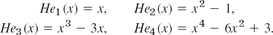
- 14. TEAM PROJECT. Orthogonality on the Entire Real Axis. Hermite Polynomials.8 These orthogonal polynomials are defined He0(1) = 1 by and

REMARK. As is true for many special functions, the literature contains more than one notation, and one sometimes defines as Hermite polynomials the functions
This differs from our definition, which is preferred in applications.
(a) Small Values of n. Show that
(b) Generating Function. A generating function of the Hermite polynomials is

because Hen(x) = n! an(x). Prove this. Hint: Use the formula for the coefficients of a Maclaurin series and note that
 .
.(c) Derivative. Differentiating the generating function with respect to x, show that

(d) Orthogonality on thex-Axis needs a weight function that goes to zero sufficiently fast as x → ±∞ (Why?)
Show that the Hermite polynomials are orthogonal on −∞ < x < ∞ with respect to the weight function r(x) = e−x2/2. Hint. Use integration by parts and (21).
(e) ODEs. Show that

Using this with n − 1 instead of n and (21), show that y = Hen(x) satisfies the ODE

Show that w = e−x2/4y is a solution of Weber's equation

- 15. CAS EXPERIMENT. Fourier–Bessel Series. Use Example 2 and R = 1, so that you get the series

With the zeros α0,1α0,2, … from your CAS (see also Table A1 in App. 5).
(a) Graph the terms J0(α0,1x), …,J0(α0,10x) for 0
x 1 on common axes.(b) Write a program for calculating partial sums of (25). Find out for what f(x) your CAS can evaluate the integrals. Take two such f(x) and comment empirically on the speed of convergence by observing the decrease of the coefficients.
(c) Take f(x) = 1 in (25) and evaluate the integrals for the coefficients analytically by (21a), Sec. 5.4, with v = 1. Graph the first few partial sums on common axes.
11.7 Fourier Integral
Fourier series are powerful tools for problems involving functions that are periodic or are of interest on a finite interval only. Sections 11.2 and 11.3 first illustrated this, and various further applications follow in Chap. 12. Since, of course, many problems involve functions that are nonperiodic and are of interest on the whole x-axis, we ask what can be done to extend the method of Fourier series to such functions. This idea will lead to “Fourier integrals.”
In Example 1 we start from a special function fL of period 2L and see what happens to its Fourier series if we let L → ∞. Then we do the same for an arbitrary function fL of period 2L. This will motivate and suggest the main result of this section, which is an integral representation given in Theorem 1 below.
Consider the periodic rectangular wave fL(x) of period 2L > 2 given by

The left part of Fig. 280 shows this function for 2L = 4, 8, 16 as well as the nonperiodic function f(x), which we obtain from fL if we let L → ∞,

We now explore what happens to the Fourier coefficients of fL as L increases. Since fL is even, bn = 0 for all n. For an the Euler formulas (6), Sec. 11.2, give
![]()
This sequence of Fourier coefficients is called the amplitude spectrum of fL because |an| is the maximum amplitude of the wave an cos (nπx/L). Figure 280 shows this spectrum for the periods 2L = 4, 8, 16. We see that for increasing L these amplitudes become more and more dense on the positive wn-axis, where wn = nπ/L. Indeed, for 2L = 4, 8, 16 we have 1, 3, 7 amplitudes per “half-wave” of the function (2 sin wn) (Lwn) (dashed in the figure). Hence for 2L = 2k we have 2k − 1 − 1 amplitudes per half-wave, so that these amplitudes will eventually be everywhere dense on the positive wn-axis (and will decrease to zero).
The outcome of this example gives an intuitive impression of what about to expect if we turn from our special function to an arbitrary one, as we shall do next.
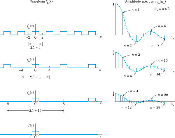
Fig. 280. Waveforms and amplitude spectra in Example 1
From Fourier Series to Fourier Integral
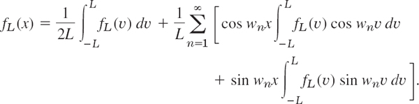
We now consider any periodic function fL(x) of period 2L that can be represented by a Fourier series

and find out what happens if we let L → ∞. Together with Example 1 the present calculation will suggest that we should expect an integral (instead of a series) involving cos wx and sin wx with w no longer restricted to integer multiples w = wn = nπ/L of π/L but taking all values. We shall also see what form such an integral might have.
If we insert an and bn from the Euler formulas (6), Sec. 11.2, and denote the variable of integration by υ, the Fourier series of fL(x) becomes
We now set
Then 1/L = Δw/π, and we may write the Fourier series in the form

This representation is valid for any fixed L, arbitrarily large, but finite.
We now let L → ∞ and assume that the resulting nonperiodic function
![]()
is absolutely integrable on the x-axis; that is, the following (finite!) limits exist:

Then 1/L→0, and the value of the first term on the right side of (1) approaches zero. Also Δw = π/L → 0 and it seems plausible that the infinite series in (1) becomes an integral from 0 to ∞, which represents f(x), namely,

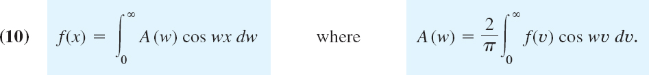
If we introduce the notations

we can write this in the form
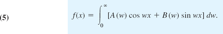
This is called a representation of f(x) by a Fourier integral.
It is clear that our naive approach merely suggests the representation (5), but by no means establishes it; in fact, the limit of the series in (1) as Δw approaches zero is not the definition of the integral (3). Sufficient conditions for the validity of (5) are as follows.
If f(x) is piecewise continuous (see Sec. 6.1) in every finite interval and has a right-hand derivative and a left-hand derivative at every point (see Sec 11.1) and if the integral (2)exists, then f(x) can be represented by a Fourier integral (5) with A and B given by (4). At a point where f(x) is discontinuous the value of the Fourier integral equals the average of the left- and right-hand limits of f(x) at that point (see Sec. 11.1). (Proof in Ref. [C12]; see App. 1.)
Applications of Fourier Integrals
The main application of Fourier integrals is in solving ODEs and PDEs, as we shall see for PDEs in Sec. 12.6. However, we can also use Fourier integrals in integration and in discussing functions defined by integrals, as the next example.
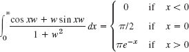
EXAMPLE 2 Single Pulse, Sine Integral. Dirichlet's Discontinuous Factor. Gibbs Phenomenon
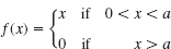
Find the Fourier integral representation of the function


Fig. 281. Example 2

and (5) gives the answer

The average of the left- and right-hand limits of f(x) at x = 1 is equal to (1 + 0)/2, that is, ![]() .
.
Furthermore, from (6) and Theorem 1 we obtain (multiply by π/2)

We mention that this integral is called Dirichlet's discontinous factor. (For P. L. Dirichlet see Sec. 10.8.)
The case x = 0 is of particular interest. If x = 0, then (7) gives

We see that this integral is the limit of the so-called sine integral
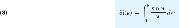
as u → ∞. The graphs of and of the integrand are shown in Fig. 282.
In the case of a Fourier series the graphs of the partial sums are approximation curves of the curve of the periodic function represented by the series. Similarly, in the case of the Fourier integral (5), approximations are obtained by replacing ∞ by numbers a. Hence the integral

approximates the right side in (6) and therefore f(x).
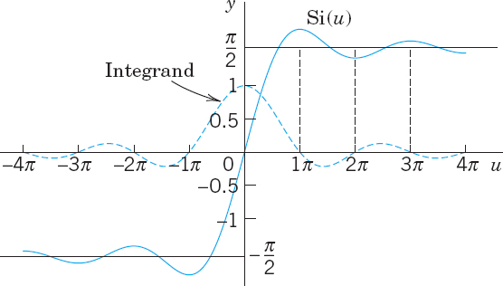
Fig. 282. Sine integral Si(u) and integrand

Fig. 283. The integral (9) for a = 8, 16, and 32, illustrating the development of the Gibbs phenomenon
Figure 283 shows oscillations near the points of discontinuity of f(x). We might expect that these oscillations disappear as a approaches infinity. But this is not true; with increasing a, they are shifted closer to the points x = ±1. This unexpected behavior, which also occurs in connection with Fourier series (see Sec. 11.2), is known as the Gibbs phenomenon. We can explain it by representing (9) in terms of sine integrals as follows. Using (11) in App. A3.1, we have

In the first integral on the right we set w + wx = t. Then dw/w = dt/t, and 0 ![]() w
w ![]() a corresponds to 0
a corresponds to 0 ![]() t
t ![]() (x + 1)a. In the last integral we set w − wx = −t. Then dw/w = dt/t, and 0
(x + 1)a. In the last integral we set w − wx = −t. Then dw/w = dt/t, and 0 ![]() w
w ![]() a corresponds to 0
a corresponds to 0 ![]() t
t ![]() (x − 1)a. Since sin(−t) = −sin t, we thus obtain
(x − 1)a. Since sin(−t) = −sin t, we thus obtain

From this and (8) we see that our integral (9) equals
![]()
and the oscillations in Fig. 283 result from those in Fig. 282. The increase of a amounts to a transformation of the scale on the axis and causes the shift of the oscillations (the waves) toward the points of discontinuity −1 and 1.
Fourier Cosine Integral and Fourier Sine Integral
Just as Fourier series simplify if a function is even or odd (see Sec. 11.2), so do Fourier integrals, and you can save work. Indeed, if f has a Fourier integral representation and is even, then B(w) = 0 in (4). This holds because the integrand of B(w) is odd. Then (5) reduces to a Fourier cosine integral
Note the change in A(w): for even f the integrand is even, hence the integral from −∞ to equals ∞ twice the integral from 0 to ∞, just as in (7a) of Sec. 11.2.
Similarly, if f has a Fourier integral representation and is odd, then A(w) = 0 in (4). This is true because the integrand of A(w) is odd. Then (5) becomes a Fourier sine integral

Note the change of B(w) to an integral from 0 to ∞ because B(w) is even (odd times odd is even).
Earlier in this section we pointed out that the main application of the Fourier integral representation is in differential equations. However, these representations also help in evaluating integrals, as the following example shows for integrals from 0 to ∞.
We shall derive the Fourier cosine and Fourier sine integrals of f(x) = e−kx, where x > 0 and k > 0 (Fig. 284). The result will be used to evaluate the so-called Laplace integrals.

Fig. 284. f(x) in Example 3
Solution. (a) From (10) we have ![]() cos wv dυ. Now, by integration by parts,
cos wv dυ. Now, by integration by parts,

If υ = 0, the expression on the right equals −k(k2 + w2). If υ approaches infinity, that expression approaches zero because of the exponential factor. Thus 2/π times the integral from 0 to ∞ gives

By substituting this into the first integral in (10) we thus obtain the Fourier cosine integral representation

From this representation we see that

(b) Similarly, from (11) we have ![]() sin wυ dυ. By integration by parts,
sin wυ dυ. By integration by parts,

This equals −w/(k2 + w2) if υ = 0, and approaches 0 as υ → ∞. Thus

From (14) we thus obtain the Fourier sine integral representation

From this we see that

The integrals (13) and (15) are called the Laplace integrals.
1–6 EVALUATION OF INTEGRALS
Show that the integral represents the indicated function. Hint. Use (5), (10), or (11); the integral tells you which one, and its value tells you what function to consider. Show your work in detail.

7–12 FOURIER COSINE INTEGRAL REPRESENTATIONS
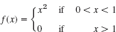
Represent f(x) as an integral (10).
- 7.

- 8.
- 9. f(x) = 1/(1 + x2) [x>0. Hint. See (13).]
- 10.

- 11.
- 12.

- 13. CAS EXPERIMENT. Approximate Fourier Cosine Integrals. Graph the integrals in Prob. 7, 9, and 11 as functions of x. Graph approximations obtained by replacing ∞ with finite upper limits of your choice. Compare the quality of the approximations. Write a short report on your empirical results and observations.
- 14. PROJECT. Properties of Fourier Integrals
(a) Fourier cosine integral. Show that (10) implies
(a1)

(a2)
(a3)

(b) Solve Prob. 8 by applying (a3) to the result of Prob. 7.
(c) Verify (a2) for f(x) = 1 if 0 < x < a and f(x) = 0 if x > a.
(d) Fourier sine integral. Find formulas for the Fourier sine integral similar to those in (a).
- 15. CAS EXPERIMENT. Sine Integral. Plot Si(u) for positive u. Does the sequence of the maximum and minimum values give the impression that it converges and has the limit π/2? Investigate the Gibbs phenomenon graphically.
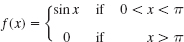
16–20 FOURIER SINE INTEGRAL REPRESENTATIONS
Represent f(x) as an integral (11).
- 16.
- 17.
- 18.

- 19.

- 20.

11.8 Fourier Cosine and Sine Transforms
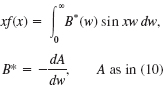
An integral transform is a transformation in the form of an integral that produces from given functions new functions depending on a different variable. One is mainly interested in these transforms because they can be used as tools in solving ODEs, PDEs, and integral equations and can often be of help in handling and applying special functions. The Laplace transform of Chap. 6 serves as an example and is by far the most important integral transform in engineering.
Next in order of importance are Fourier transforms. They can be obtained from the Fourier integral in Sec. 11.7 in a straightforward way. In this section we derive two such transforms that are real, and in Sec. 11.9 a complex one.
Fourier Cosine Transform
The Fourier cosine transform concerns even functions f(x). We obtain it from the Fourier cosine integral [(10) in Sec. 10.7]

Namely, we set ![]() , where c suggests “cosine.” Then, writing υ = x in the formula for A(w), we have
, where c suggests “cosine.” Then, writing υ = x in the formula for A(w), we have

and

Formula (1a) gives from f(x) a new function ![]() , called the Fourier cosine transform of f (x). Formula (1b) gives us back f(x) from
, called the Fourier cosine transform of f (x). Formula (1b) gives us back f(x) from ![]() , and we therefore call f(x) the inverse Fourier cosine transform of
, and we therefore call f(x) the inverse Fourier cosine transform of ![]() .
.
The process of obtaining the transform ![]() from a given f is also called the Fourier cosine transform or the Fourier cosine transform method.
from a given f is also called the Fourier cosine transform or the Fourier cosine transform method.
Fourier Sine Transform
Similarly, in (11), Sec. 11.7, we set ![]() , where s suggests “sine.” Then, writing υ = x we have from (11), Sec. 11.7, the Fourier sine transform, of f(x) given by
, where s suggests “sine.” Then, writing υ = x we have from (11), Sec. 11.7, the Fourier sine transform, of f(x) given by

and the inverse Fourier sine transform of ![]() , given by
, given by
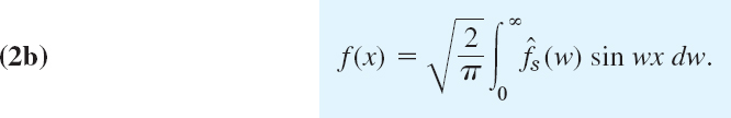
The process of obtaining fs(w) from f(x) is also called the Fourier sine transform or the Fourier sine transform method.
Other notations are

and ![]() and
and ![]() for the inverses of
for the inverses of ![]() and
and ![]() , respectively.
, respectively.
EXAMPLE 1 Fourier Cosine and Fourier Sine Transforms
Find the Fourier cosine and Fourier sine transforms of the function


Fig. 285. f(x) in Example 1
Solution. From the definitions (1a) and (2a) we obtain by integration
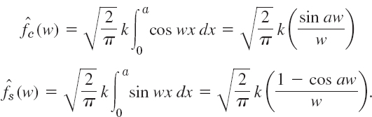
This agrees with formulas 1 in the first two tables in Sec. 11.10 (where k = 1).
Note that for f(x) = k = const (0 < x < ∞), these transforms do not exist. (Why?)
EXAMPLE 2 Fourier Cosine Transform of the Exponential Function
Find ![]() .
.
Solution. By integration by parts and recursion,

This agrees with formula 3 in Table I, Sec. 11.10, with a = 1. See also the next example.
What did we do to introduce the two integral transforms under consideration? Actually not much: We changed the notations A and B to get a “symmetric” distribution of the constant 2/π in the original formulas (1) and (2). This redistribution is a standard convenience, but it is not essential. One could do without it.
What have we gained? We show next that these transforms have operational properties that permit them to convert differentiations into algebraic operations (just as the Laplace transform does). This is the key to their application in solving differential equations.
Linearity, Transforms of Derivatives
If f(x) is absolutely integrable (see Sec. 11.7) on the positive x-axis and piecewise continuous (see Sec. 6.1) on every finite interval, then the Fourier cosine and sine transforms of f exist.
Furthermore, if f and g have Fourier cosine and sine transforms, so does af + bg for any constants a and b, and by (1a)

The right side is ![]() . Similarly for
. Similarly for ![]() , by (2). This shows that the Fourier cosine and sine transforms are linear operations,
, by (2). This shows that the Fourier cosine and sine transforms are linear operations,
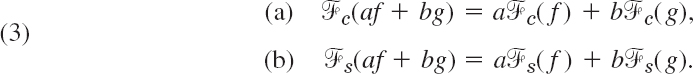
THEOREM 1 Cosine and Sine Transforms of Derivatives
Let f(x) be continuous and absolutely integrable on the x-axis, let f′(x) be piecewise continuous on every finite interval, and let f(x) → 0 as x → ∞. Then
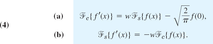
PROOF
This follows from the definitions and by using integration by parts, namely, and similarly,

and similarly,

Formula (4a) with f′ instead of f gives (when f′, f″ satisfy the respective assumptions for f, f′ in Theorem 1)
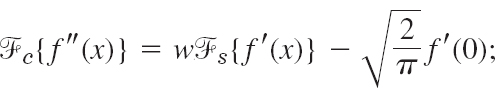
hence by (4b)

Similarly,
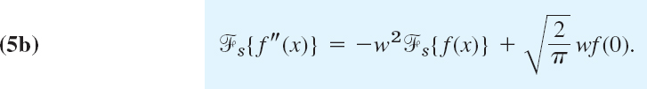
A basic application of (5) to PDEs will be given in Sec. 12.7. For the time being we show how (5) can be used for deriving transforms.
EXAMPLE 3 An Application of the Operational Formula (5)
Find the Fourier cosine transform ![]() of f(x) = e−ax, where a > 0.
of f(x) = e−ax, where a > 0.
Solution. By differentiation, (e−ax)″ = a2e−ax; thus
![]()
From this, (5a), and the linearity (3a),

Hence

The answer is (see Table I, Sec. 11.10)

Tables of Fourier cosine and sine transforms are included in Sec. 11.10.
1–8 FOURIER COSINE TRANSFORM
- Find the cosine transform
 of f(x) = 1 if 0 < x < 1, f(x) = −1 if 1 < x < 2, f(x) = 0 if x > 2.
 - Find f in Prob. 1 from the answer
 .
. - Find for f(x) = x if 0 < x < 2, f(x) = 0 if x > 2.
- Derive formula 3 in Table I of Sec. 11.10 by integration.
- Find for f(x) = x2 if 0 < x < 1, f(x) = 0 if x > 1.
- Continuity assumptions. Find
 for g(x) = 2 if 0 < x < 1, g(x) = 0 if x > 1. Try to obtain from it for f(x) in Prob. 5 by using (5a).
 - Existence? Does the Fourier cosine transform of x−1 sin x (0 < x < ∞) exist? Of x−1 cos x? Give reasons.
- Existence? Does the Fourier cosine transform of f(x) = k = const (0 < x < ∞) exist? The Fourier sine transform?
9–15 FOURIER SINE TRANSFORM
- 9. Find
 , a > 0, by integration.
 - 10. Obtain the answer to Prob. 9 from (5b).
- 11. Find fs(w) for f(x) = x2 if 0 < x < 1, f(x) = 0 if x > 1.
- 12. Find
 from (4b) and a suitable formula in Table I of Sec. 11.10.
 - 13. Find from (4a) and formula 3 of Table I in Sec. 11.10.
- 14. Gamma function. Using formulas 2 and 4 in Table II of Sec. 11.10, prove
 in App. A3.1], a value needed for Bessel functions and other applications.
 - 15. WRITING PROJECT. Finding Fourier Cosine and Sine Transforms. Write a short report on ways of obtaining these transforms, with illustrations by examples of your own.
11.9 Fourier Transform. Discrete and Fast Fourier Transforms
In Sec. 11.8 we derived two real transforms. Now we want to derive a complex transform that is called the Fourier transform. It will be obtained from the complex Fourier integral, which will be discussed next.
Complex Form of the Fourier Integral
The (real) Fourier integral is [see (4), (5), Sec. 11.7]

where

Substituting A and B into the integral for f, we have
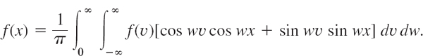
By the addition formula for the cosine [(6) in App. A3.1] the expression in the brackets […] equals cos (wx − wυ) or, since the cosine is even, cos (wx − wυ). We thus obtain
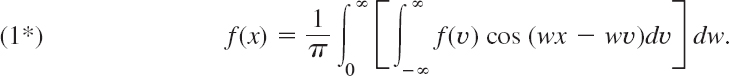
The integral in brackets is an even function of w, call it F(w), bacause cos (wx − wυ) is an even function of w the function f does not depend on w, and we integrate with respect to υ (not w). Hence the integral of F(w) from w = 0 to ∞ is ![]() times the integral of F(w) from −∞ to ∞. Thus (note the change of the integration limit!)
times the integral of F(w) from −∞ to ∞. Thus (note the change of the integration limit!)

We claim that the integral of the form (1) with sin instead of cos is zero:

This is true since sin (wx − wυ) is an odd function of w, which makes the integral in brackets an odd function of w, call it G(w). Hence the integral of G(w) from −∞ to ∞ is zero, as claimed.
We now take the integrand of (1) plus ![]() times the integrand of (2) and use the Euler formula [(11) in Sec. 2.2]
times the integrand of (2) and use the Euler formula [(11) in Sec. 2.2]
![]()
Taking wx − wυ instead of x in (3) and multiplying by f(υ) gives
![]()
Hence the result of adding (1) plus i times (2), called the complex Fourier integral, is

To obtain the desired Fourier transform will take only a very short step from here.
Fourier Transform and Its Inverse
Writing the exponential function in (4) as a product of exponential functions, we have

The expression in brackets is a function of w, is denoted by ![]() , and is called the Fourier transform of f; writing υ = x, we have
, and is called the Fourier transform of f; writing υ = x, we have
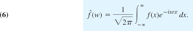

and is called the inverse Fourier transform of ![]() .
.
Another notation for the Fourier transform is

so that
![]()
The process of obtaining the Fourier transform ![]() from a given f is also called the Fourier transform or the Fourier transform method.
from a given f is also called the Fourier transform or the Fourier transform method.
Using concepts defined in Secs. 6.1 and 11.7 we now state (without proof) conditions that are sufficient for the existence of the Fourier transform.
THEOREM 1 Existence of the Fourier Transform
If is absolutely integrable on the x-axis and piecewise continuous on every finite interval, then the Fourier transform ![]() of f(x) given by (6) exists.
of f(x) given by (6) exists.
Find the Fourier transform of f(x) = 1 if |x| < 1 and f(x) = 0 otherwise.
Solution. Using (6) and integrating, we obtain

As in (3) we have eiw = cos w + i sin w, e−iw = cos w − i sin w, and by subtraction
![]()
Substituting this in the previous formula on the right, we see that i drops out and we obtain the answer

Find the Fourier transform ![]() of f(x) = e−ax if x > 0 and f(x) = 0 if x < 0; here a > 0.
of f(x) = e−ax if x > 0 and f(x) = 0 if x < 0; here a > 0.
Solution. From the definition (6) we obtain by integration

This proves formula 5 of Table III in Sec. 11.10.
Physical Interpretation: Spectrum
The nature of the representation (7) of f(x) becomes clear if we think of it as a superposition of sinusoidal oscillations of all possible frequencies, called a spectral representation. This name is suggested by optics, where light is such a superposition of colors (frequencies). In (7), the “spectral density” ![]() measures the intensity of f(x) in the frequency interval between w and w + Δw (Δw small, fixed). We claim that, in connection with vibrations, the integral
measures the intensity of f(x) in the frequency interval between w and w + Δw (Δw small, fixed). We claim that, in connection with vibrations, the integral

can be interpreted as the total energy of the physical system. Hence an integral of ![]() from a to b gives the contribution of the frequencies w between a and b to the total energy.
from a to b gives the contribution of the frequencies w between a and b to the total energy.
To make this plausible, we begin with a mechanical system giving a single frequency, namely, the harmonic oscillator (mass on a spring, Sec. 2.4)
![]()
Here we denote time t by x. Multiplication by y′ gives my′ y″ + ky′y = 0. By integration,
![]()
where υ = y′ is the velocity. The first term is the kinetic energy, the second the potential energy, and the total energy of the system. Now a general solution is (use (3) in Sec. 11.4 with t = x)
![]()
where ![]() . We write simply A = c1eiw0x, B = c−1e−iw0x. Then y = A + B. By differentiation, υ = y′ = A′ + B′ = iw0(A − B). Substitution of υ and y on the left side of the equation for E0 gives
. We write simply A = c1eiw0x, B = c−1e−iw0x. Then y = A + B. By differentiation, υ = y′ = A′ + B′ = iw0(A − B). Substitution of υ and y on the left side of the equation for E0 gives
![]()
Here ![]() , as just stated; hence
, as just stated; hence ![]() . Also i2 = −1, so that
. Also i2 = −1, so that
![]()
Hence the energy is proportional to the square of the amplitude |c1|.
As the next step, if a more complicated system leads to a periodic solution y = f(x) that can be represented by a Fourier series, then instead of the single energy term |c1|2 we get a series of squares |cn|2 of Fourier coefficients cn given by (6), Sec. 11.4. In this case we have a “discrete spectrum” (or “point spectrum”) consisting of countably many isolated frequencies (infinitely many, in general), the corresponding |cn|2 being the contributions to the total energy.
Finally, a system whose solution can be represented by an integral (7) leads to the above integral for the energy, as is plausible from the cases just discussed.
Linearity. Fourier Transform of Derivatives
New transforms can be obtained from given ones by using
THEOREM 2 Linearity of the Fourier Transform
The Fourier transform is a linear operation ; that is, for any functions f(x) and g(x) whose Fourier transforms exist and any constants a and b, the Fourier transform of af + bg exists, and

PROOF
This is true because integration is a linear operation, so that (6) gives

In applying the Fourier transform to differential equations, the key property is that differentiation of functions corresponds to multiplication of transforms by iw:
THEOREM 3 Fourier Transform of the Derivative of f(x)
Let be continuous on the x-axis and f(x) → 0 as |x| → ∞. Furthermore, let f′(x) be absolutely integrable on the x-axis. Then
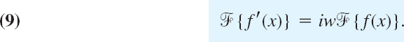
PROOF
From the definition of the Fourier transform we have

Integrating by parts, we obtain

Since f(x) → 0 as |x| → ∞, the desired result follows, namely,
![]()
Two successive applications of (9) give
![]()
Since (iw)2 = −w2 we have for the transform of the second derivative of f
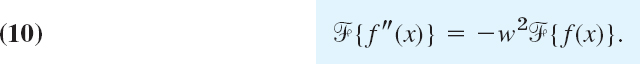
Similarly for higher derivatives.
An application of (10) to differential equations will be given in Sec. 12.6. For the time being we show how (9) can be used to derive transforms.
EXAMPLE 3 Application of the Operational Formula (9)
Find the Fourier transform of xe−x2 from Table III, Sec 11.10.
Solution. We use (9). By formula 9 in Table III

Convolution
The convolution f * g of functions f and g is defined by

The purpose is the same as in the case of Laplace transforms (Sec. 6.5): taking the convolution of two functions and then taking the transform of the convolution is the same as multiplying the transforms of these functions (and multiplying them by ![]() ):
):
Suppose that and g(x) are piecewise continuous, bounded, and absolutely integrable on the x-axis. Then

By the definition,

An interchange of the order of integration gives

Instead of x we now take x − p = q as a new variable of integration. Then x = p + q and

This double integral can be written as a product of two integrals and gives the desired result

By taking the inverse Fourier transform on both sides of (12), writing ![]() and
and ![]() as before, and noting that
as before, and noting that ![]() and 1/
and 1/![]() in (12) and (7) cancel each other, we obtain
in (12) and (7) cancel each other, we obtain
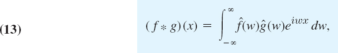
a formula that will help us in solving partial differential equations (Sec. 12.6).
Discrete Fourier Transform (DFT), Fast Fourier Transform (FFT)
In using Fourier series, Fourier transforms, and trigonometric approximations (Sec. 11.6) we have to assume that a function f(x), to be developed or transformed, is given on some interval, over which we integrate in the Euler formulas, etc. Now very often a function f(x) is given only in terms of values at finitely many points, and one is interested in extending Fourier analysis to this case. The main application of such a “discrete Fourier analysis” concerns large amounts of equally spaced data, as they occur in telecommunication, time series analysis, and various simulation problems. In these situations, dealing with sampled values rather than with functions, we can replace the Fourier transform by the so-called discrete Fourier transform (DFT) as follows.
Let f(x) be periodic, for simplicity of period 2π. We assume that N measurements of f(x) are taken over the interval 0 ![]() x
x ![]() 2π at regularly spaced points
2π at regularly spaced points

We also say that f(x) is being sampled at these points. We now want to determine a complex trigonometric polynomial

that interpolates f(x) at the nodes (14), that is, q(xk) = f(xk) written out, with fk denoting f(xk)

Hence we must determine the coefficients c0, …,cN−1 such that (16) holds. We do this by an idea similar to that in Sec. 11.1 for deriving the Fourier coefficients by using the orthogonality of the trigonometric system. Instead of integrals we now take sums. Namely, we multiply (16) by e−imxk (note the minus!) and sum over k from 0 to N − 1. Then we interchange the order of the two summations and insert xk from (14). This gives

Now
![]()
We donote […] by r. For n = w we have r = e0 = 1. The sum of these terms over k equals N, the number of these terms. For n ≠ m we have r ≠ 1 and by the formula for a geometric sum [(6) in Sec. 15.1 with q = r and n = N − 1]
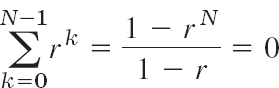
because rN = 1; indeed, since k, m, and n are integers,
![]()
This shows that the right side of (17) equals cmN. Writing n for m and dividing by N, we thus obtain the desired coefficient formula
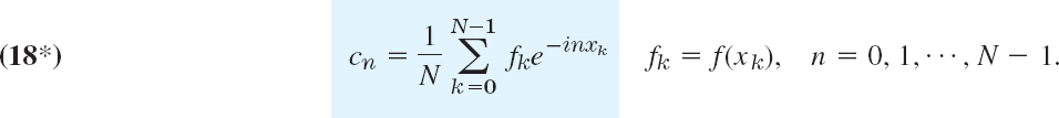
Since computation of the cn (by the fast Fourier transform, below) involves successive halfing of the problem size N, it is practical to drop the factor 1/N from cn and define the discrete Fourier transform of the given signal f = [f0 … fN−1]T to be the vector ![]() with components
with components

This is the frequency spectrum of the signal.
In vector notation, ![]() , where the N × N Fourier matrix FN = [enk] has the entries [given in (18)]
, where the N × N Fourier matrix FN = [enk] has the entries [given in (18)]
![]()
where n, k = 0, …, N − 1.
EXAMPLE 4 Discrete Fourier Transform (DFT). Sample of Values N = 4 Values
Let N = 4 measurements (sample values) be given. Then w = e−2πi/N = e−πi/2 = −i and thus wnk = (−i)nk. Let the sample values be, say f = [0 1 4 9]T. Then by (18) and (19),

From the first matrix in (20) it is easy to infer what FN looks like for arbitrary N, which in practice may be 1000 or more, for reasons given below.
From the DFT (the frequency spectrum) ![]() we can recreate the given signal
we can recreate the given signal ![]() , as we shall now prove. Here FN and its complex conjugate
, as we shall now prove. Here FN and its complex conjugate ![]() satisfy
satisfy
![]()
where I is the N × N unit matrix; hence FN has the inverse

PROOF
We prove (21). By the multiplication rule (row times column) the product matrix ![]() in (21a) has the entries gjk = Row j of
in (21a) has the entries gjk = Row j of ![]() times Column k of FN. That is, writing
times Column k of FN. That is, writing ![]() , we prove that
, we prove that

Indeed, when j = k, then ![]() , so that the sum of these N terms equals N; these are the diagonal entries of GN. Also, when j ≠ k, then W ≠ 1 and we have a geometric sum (whose value is given by (6) in Sec. 15.1 with q = W and n = N − 1)
, so that the sum of these N terms equals N; these are the diagonal entries of GN. Also, when j ≠ k, then W ≠ 1 and we have a geometric sum (whose value is given by (6) in Sec. 15.1 with q = W and n = N − 1)
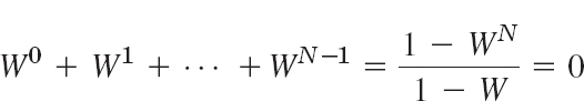
because ![]()
We have seen that ![]() is the frequency spectrum of the signal f(x). Thus the components
is the frequency spectrum of the signal f(x). Thus the components ![]() of
of ![]() give a resolution of the 2π-periodic function f(x) into simple (complex) harmonics. Here one should use only n's that are much smaller than N/2, to avoid aliasing. By this we mean the effect caused by sampling at too few (equally spaced) points, so that, for instance, in a motion picture, rotating wheels appear as rotating too slowly or even in the wrong sense. Hence in applications, N is usually large. But this poses a problem. Eq. (18) requires O(N) operations for any particular n, hence O(N2) operations for, say, all n < N/2. Thus, already for 1000 sample points the straightforward calculation would involve millions of operations. However, this difficulty can be overcome by the so-called fast Fourier transform (FFT), for which codes are readily available (e.g., in Maple). The FFT is a computational method for the DFT that needs only O(N) log2N operations instead of O(N2). It makes the DFT a practical tool for large N. Here one chooses N = 2p (p integer) and uses the special form of the Fourier matrix to break down the given problem into smaller problems. For instance, when N = 1000, those operations are reduced by a factor 1000/log2 1000 ≈ 100.
give a resolution of the 2π-periodic function f(x) into simple (complex) harmonics. Here one should use only n's that are much smaller than N/2, to avoid aliasing. By this we mean the effect caused by sampling at too few (equally spaced) points, so that, for instance, in a motion picture, rotating wheels appear as rotating too slowly or even in the wrong sense. Hence in applications, N is usually large. But this poses a problem. Eq. (18) requires O(N) operations for any particular n, hence O(N2) operations for, say, all n < N/2. Thus, already for 1000 sample points the straightforward calculation would involve millions of operations. However, this difficulty can be overcome by the so-called fast Fourier transform (FFT), for which codes are readily available (e.g., in Maple). The FFT is a computational method for the DFT that needs only O(N) log2N operations instead of O(N2). It makes the DFT a practical tool for large N. Here one chooses N = 2p (p integer) and uses the special form of the Fourier matrix to break down the given problem into smaller problems. For instance, when N = 1000, those operations are reduced by a factor 1000/log2 1000 ≈ 100.
The breakdown produces two problems of size M = N/2. This breakdown is possible because for N = 2M we have in (19)
![]()
The given vector f = [f0 … fN − 1]T is split into two vectors with M components each, namely, fev = [f0 f2 … fN−2]T containing the even components of f, and fod = [f1 f3 … fN−1]T containing the odd components of f. For fev and fod we determine the DFTs

and
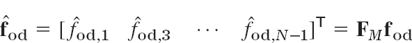
involving the same M × M matrix FM. From these vectors we obtain the components of the DFT of the given vector f by the formulas

For N = 2p this breakdown can be repeated p − 1 times in order to finally arrive at N/2 problems of size 2 each, so that the number of multiplications is reduced as indicated above.
We show the reduction from N = 4 to M = N/2 = 2 and then prove (22).
EXAMPLE 5 Fast Fourier Transform (FFT). Sample of N = 4 Values
When N = 4, then w = wN = −i as in Example 4 and M = N/2 = 2, hence w = wM = e−2πi/2 = e−πi = −1 Consequently,

From this and (22a) we obtain
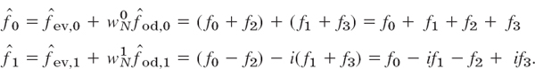
Similarly, by (22b),

This agrees with Example 4, as can be seen by replacing 0, 1, 4, 9 with f0, f1, f2, f3
We prove (22). From (18) and (19) we have for the components of the DFT
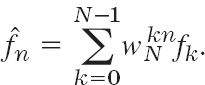
Splitting into two sums of M = N/2 terms each gives

We now use ![]() and pull out
and pull out ![]() from under the second sum, obtaining
from under the second sum, obtaining

The two sums are fev,n and fod,n, the components of the “half-size” transforms Ffev and Ffod.
Formula (22a) is the same as (23). In (22b) we have n + M instead of n. This causes a sign changes in (23), namely −![]() before the second sum because
before the second sum because
![]()
This gives the minus in (22b) and completes the proof.
- Review in complex. Show that 1/i = −i, e−ix = cos x − i sin x, eix + e−ix = 2 cos x, eix − e−ix = 2i sin x, eikx = cos kx + i sin kx.
2–11 FOURIER TRANSFORMS BY INTEGRATION
Find the Fourier transform of f(x) (without using Table III in Sec. 11.10). Show details.
- 2.

- 3.

- 4.

- 5.

- 6. f(x) = e−|x| (−∞ < x < ∞)
- 7.

- 8.

- 9.
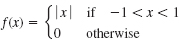
- 10.

- 11.

12–17 USE OF TABLE III IN SEC. 11.10. OTHER METHODS
- 12. Find
 for f(x) = xe−x if x > 0, f(x) = 0 if x < 0, by (9) in the text and formula 5 in Table III (with a = 1). Hint. Consider xe−x and e−x.
 - 13. Obtain
 from Table III.
 - 14. In Table III obtain formula 7 from formula 8.
- 15. In Table III obtain formula 1 from formula 2.
- 16. TEAM PROJECT. Shifting (a) Show that if f(x) has a Fourier transform, so does f(x − a), and
 .
.
(b) Using (a), obtain formula 1 in Table III, Sec. 11.10, from formula 2.
(c) Shifting on the w-Axis. Show that if
 is the Fourier transform of f(x), then
  is the Fourier transform of eiaxf(x).
(d) Using (c), obtain formula 7 in Table III from 1 and formula 8 from 2.
- 17. What could give you the idea to solve Prob. 11 by using the solution of Prob. 9 and formula (9) in the text? Would this work?
18–25 DISCRETE FOURIER TRANSFORM
- 18. Verify the calculations in Example 4 of the text.
- 19. Find the transform of a general f = [f1 f2 f3 f4]T signal of four values.
- 20. Find the inverse matrix in Example 4 of the text and use it to recover the given signal.
- 21. Find the transform (the frequency spectrum) of a general signal of two values [f1 f2]T.
- 22. Recreate the given signal in Prob. 21 from the frequency spectrum obtained.
- 23. Show that for a signal of eight sample values,
 . Check by squaring.
 - 24. Write the Fourier matrix F for a sample of eight values explicitly.
- 25. CAS Problem. Calculate the inverse of the 8×8 Fourier matrix. Transform a general sample of eight values and transform it back to the given data.
11.10 Tables of Transforms
Table I. Fourier Cosine Transforms
See (2) in Sec. 11.8.
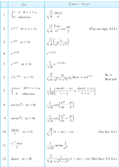
Table II. Fourier Sine Transforms
See (5) in Sec. 11.8.

Table III. Fourier Transforms
See (6) in Sec. 11.9.
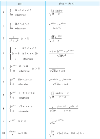
CHAPTER 11 REVIEW QUESTIONS AND PROBLEMS
- What is a Fourier series? A Fourier cosine series? A half-range expansion? Answer from memory.
- What are the Euler formulas? By what very important idea did we obtain them?
- How did we proceed from 2π-periodic to general-periodic functions?
- Can a discontinuous function have a Fourier series? A Taylor series? Why are such functions of interest to the engineer?
- What do you know about convergence of a Fourier series? About the Gibbs phenomenon?
- The output of an ODE can oscillate several times as fast as the input. How come?
- What is approximation by trigonometric polynomials? What is the minimum square error?
- What is a Fourier integral? A Fourier sine integral? Give simple examples.
- What is the Fourier transform? The discrete Fourier transform?
- What are Sturm–Liouville problems? By what idea are they related to Fourier series?
11–20 FOURIER SERIES. In Probs. 11, 13, 16, 20 find the Fourier series of f(x) as given over one period and sketch f(x) and partial sums. In Probs. 12, 14, 15, 17–19 give answers, with reasons. Show your work detail.
- 11.

- 12. Why does the series in Prob. 11 have no cosine terms?
- 13.

- 14. What function does the series of the cosine terms in Prob. 13 represent? The series of the sine terms?
- 15. What function do the series of the cosine terms and the series of the sine terms in the Fourier series of ex(−5 < x < 5) represent?
- 16. f(x) = |x| (−π < x < π)
- 17. Find a Fourier series from which you can conclude that 1 − 1/3 + 1/5 − 1/7 + −… = π/4.
- 18. What function and series do you obtain in Prob. 16 by (termwise) differentiation?
- 19. Find the half-range expansions of f(x) = x (0 < x < 1).
- 20. f(x) = 3x2 (−π < x < π)
21–22 GENERAL SOLUTION
Solve, y″ + ω2y = r(t), where |ω| ≠ 0, 1, 2, …, r(t) is 2π-periodic and
- 21. r(t) = 3t2 (−π < t < π)
- 22. r(t) = |t| (−π < t < π)
23–25 MINIMUM SQUARE ERROR
- 23. Compute the minimum square error for f(x) = x/π (−π < x < π) and trigonometric polynomials of degree N = 1, …, 5.
- 24. How does the minimum square error change if you multiply f(x) by a constant k?
- 25. Same task as in Prob. 23, for f(x) = |x|/π (−π < x < π). Why is E* now much smaller (by a factor 100, approximately!)?
26–30 FOURIER INTEGRALS AND TRANSFORMS
Sketch the given function and represent it as indicated. If you have a CAS, graph approximate curves obtained by replacing ∞ with finite limits; also look for Gibbs phenomena.
- 26. f(x) = x + 1 if 0 < x < 1 and 0 otherwise; by the Fourier sine transform
- 27. f(x) = x if 0 < x < 1 and 0 otherwise; by the Fourier integral
- 28. f(x) = kx if a < x < b and 0 otherwise; by the Fourier transform
- 29. f(x) = x if 1 < x < a and 0 otherwise; by the Fourier cosine transform
- 30. f(x) = e−2x if x > 0 and 0 otherwise; by the Fourier transform
SUMMARY OF CHAPTER 11 Fourier Analysis. Partial Differential Equations (PDEs)
Fourier series concern periodic functions f(x) of period p = 2L, that is, by definition f(x + p) = f(x) for all x and some fixed p > 0; thus, f(x + np) = f(x) for any integer n. These series are of the form

with coefficients, called the Fourier coefficients of f(x), given by the Euler formulas (Sec. 11.2)

where n = 1, 2, …. For period 2π we simply have (Sec. 11.1)
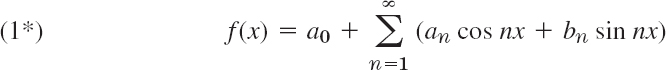
with the Fourier coefficients of f(x) (Sec. 11.1)

Fourier series are fundamental in connection with periodic phenomena, particularly in models involving differential equations (Sec. 11.3, Chap, 12). If f(x) is even [f(−x) = f(x)] or odd [f(−x) = −f(x)], they reduce to Fourier cosine or Fourier sine series, respectively (Sec. 11.2). If f(x) is given for 0 ![]() x
x ![]() L only, it has two half-range expansions of period 2L, namely, a cosine and a sine series (Sec. 11.2).
L only, it has two half-range expansions of period 2L, namely, a cosine and a sine series (Sec. 11.2).
The set of cosine and sine functions in (1) is called the trigonometric system. Its most basic property is its orthogonality on an interval of length 2L; that is, for all integers m and n ≠ m we have

and for all integers m and n,
This orthogonality was crucial in deriving the Euler formulas (2).
Partial sums of Fourier series minimize the square error (Sec. 11.4).
Replacing the trigonometric system in (1) by other orthogonal systems first leads to Sturm–Liouville problems (Sec. 11.5), which are boundary value problems for ODEs. These problems are eigenvalue problems and as such involve a parameter λ that is often related to frequencies and energies. The solutions to Sturm–Liouville problems are called eigenfunctions. Similar considerations lead to other orthogonal series such as Fourier–Legendre series and Fourier–Bessel series classified as generalized Fourier series (Sec. 11.6).
Ideas and techniques of Fourier series extend to nonperiodic functions f(x) defined on the entire real line; this leads to the Fourier integral

where

or, in complex form (Sec. 11.9),

where

Formula (6) transforms f(x) into its Fourier transform ![]() , and (5) is the inverse transform.
, and (5) is the inverse transform.
Related to this are the Fourier cosine transform (Sec. 11.8)

and the Fourier sine transform (Sec. 11.8)
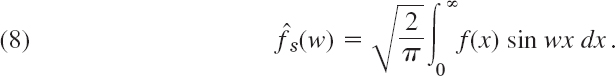
The discrete Fourier transform (DFT) and a practical method of computing it, called the fast Fourier transform (FFT), are discussed in Sec. 11.9.
2The left-hand limit of f(x) at x0 is defined as the limit of f(x) as x approaches x0 from the left and is commonly denoted by f(x0 − 0). Thus
![]()
The right-hand limit is denoted by f(x0 + 0) and
![]()
The left- and right-hand derivatives of f(x) at x0 are defined as the limits of
![]()
respectively, as h → 0 through positive values. Of course if f(x) is continuous at x0, the last term in both numerators is simply f(x0)
3MARC ANTOINE PARSEVAL (1755–1836), French mathematician. A physical interpretation of the identity follows in the next section.
4JACQUES CHARLES FRANÇOIS STURM (1803–1855) was born and studied in Switzerland and then moved to Paris, where he later became the successor of Poisson in the chair of mechanics at the Sorbonne (the University of Paris).
JOSEPH LIOUVILLE (1809–1882), French mathematician and professor in Paris, contributed to various fields in mathematics and is particularly known by his important work in complex analysis (Liouville's theorem; Sec. 14.4), special functions, differential geometry, and number theory.
5LEOPOLD KRONECKER (1823–1891). German mathematician at Berlin University, who made important contributions to algebra, group theory, and number theory.
6PAFNUTI CHEBYSHEV (1821–1894), Russian mathematician, is known for his work in approximation theory and the theory of numbers. Another transliteration of the name is TCHEBICHEF.
7EDMOND LAGUERRE (1834–1886), French mathematician, who did research work in geometry and in the theory of infinite series.
8CHARLES HERMITE (1822–1901), French mathematician, is known for his work in algebra and number theory. The great HENRI POINCARÉ (1854–1912) was one of his students.