5.3 Pose Measurement Methods
In the following the main methodologies are introduced showing how sensors are used to estimate robot pose in the environment. Those approaches can measure relative pose advancement according to previously determined pose or absolute pose according to some reference-based coordinate system.
5.3.1 Dead Reckoning
Dead reckoning (also called deduced reckoning) approaches estimate the robot’s (equipped with relative sensors) current pose from the known previous pose and relative measured displacements from the previous pose. Those displacements or motion increments (distance and orientation) are calculated from measured speeds over the elapsed time and heading. Common to those approaches is the use of path integration to estimate the current pose; therefore, the accumulation of different errors (error of integration method, measurement error, bias, noise, etc.) typically appears.
The two basic approaches used in mobile robotics are odometry and inertial navigation.
Odometry
Odometry is used to estimate the robot pose by integration of motion increments that can be measured or gathered from applied motion commands. Relative motion increments are in mobile robotics usually obtained from axis sensors (e.g., incremental encoder) that are attached to the robot’s wheels. Using an internal kinematic model (see Eq. 2.1 for differential drive) these wheel rotation measurements are related to the position and the orientation changes of the mobile robot. The position and orientation changes given in the known time period between successive measurements can also be expressed by robot velocities. In some cases wheel angular velocities can be measured directly or inferred from known velocity commands (supposing that implemented speed controllers are accurate).
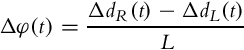
Let us assume there is a robot with differential drive and incremental encoder sensors mounted on the wheels. The measurements give relative rotation change of the left and right wheel, namely ΔαL(t) and ΔαR(t), from the previous orientation at time t− = t −Δt. Supposing that there is pure rolling of the wheels the traveled distances are
where R is the wheel’s radius. Using the internal kinematic model (2.1) orientation displacement and traveled distance (position displacements) are
and
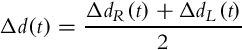
where L is the distance between the wheels.
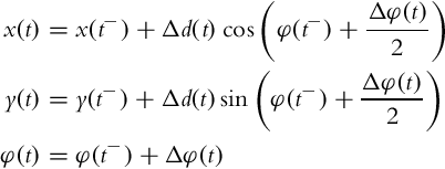
The robot pose estimate is obtained by integration of the external kinematic model (2.2) from measured robot velocities or as a summation of calculated robot position and orientation displacements. Applying trapezoidal numerical integration the estimated robot pose is
However, due to the integral nature of odometry, cumulative error occurs. The main source of the error consists of the systematic and nondeterministic error sources. The former includes errors due to approximate kinematic models (e.g., wrong radius of the wheel), error due to accuracy of applied integration method, and measurement error (unknown bias), and the latter includes slippage of the wheels, noise, and the like. Therefore, independent use of odometry is applicable only for short-term pose estimation at a known initial pose. More commonly, odometry is used in combination with pose measurements from absolute sensors where odometry is used for prediction and filtration of absolute pose measurements to obtain better pose estimates.
In wheeled mobile systems sensors used in odometry usually are axis sensors (e.g., incremental optical or magnetic encoders, potentiometers) that are attached to the wheels’ axes and measure rotation angle or velocity.
Inertial Navigation
An inertial navigation system (INS) is a self-contained technique to estimate vehicle position, orientation, and velocity by means of dead reckoning. INS includes motion sensors (accelerometers) and rotation sensors (gyroscopes) where position and orientation of the vehicle is estimated relatively to a known initial starting pose.
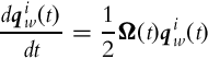
Output of accelerometer and gyroscope measurements are 3D vectors of accelerations and angular velocities in space. To estimate robot position and orientation double integration of acceleration measurement and single integration of angular velocity is required. Use of integration is the main cause for pose error of INSs because of accumulation of constant (systematic) errors (sensor drift, bad sensor calibration, etc.). Constant measurement error causes quadratic growth of the position estimate error with time while the error of orientation estimate grows linearly with time. Additionally the error of position estimate in INS is dependent on the error of orientation estimate because the accelerometer measures total acceleration including gravitation. Vehicle (INS unit) acceleration is obtained from acceleration measurement by subtracting gravity acceleration, which requires the accurate knowledge of the vehicle orientation. Any error in orientation therefore causes incorrect virtual acceleration due to inexact gravity canceling. This is especially problematic because vehicle accelerations are usually much smaller than gravity. A small signal-to-noise ratio (SNR) at lower accelerations causes additional troubles. These effects are clearly seen from the acceleration sensor model consisting of translational vehicle acceleration a, gravity g = [0, 0, 0.981]T, and radial acceleration,
where am is the acceleration measurement from a sensor in its local coordinates, ![]() is the rotation matrix between Earth’s coordinates and world coordinates where pose tracking is performed,
is the rotation matrix between Earth’s coordinates and world coordinates where pose tracking is performed, ![]() is the rotation matrix from the local INS coordinates to the world coordinates, ω is angular velocity in world coordinates, v is translational velocity, abias is acceleration bias, and anoise is noise.
is the rotation matrix from the local INS coordinates to the world coordinates, ω is angular velocity in world coordinates, v is translational velocity, abias is acceleration bias, and anoise is noise.
To estimate orientation a gyroscope measurement is used. The model of a gyroscope sensor is
where ωm is a vector of measured angular rates, ωi is a true vector of angular rates of the body in local coordinates, ωbias is sensor bias, and ωnoise is sensor noise.
To estimate INS unit orientation the unit angular rate estimates are obtained from Eq. (5.61) as follows: ωi =ωm −ωbias. The biased part is usually estimated online by means of some estimator (e.g., Kalman filter). Exceptionally, for shorter estimation periods, the bias can be supposed constant if quality gyroscope is used and initial calibration (estimation of ωbias) is made. Note, however, that bias is changing with time. Therefore, the latter approach is sufficient for short-term use only. The simplest calibration may be obtained by averaging the gyroscope measurement (for N measurements) while holding the INS unit in a constant position (![]() , when ωi = 0).
, when ωi = 0).
A relative estimate of INS unit orientation according to initial orientation is then obtained using rotational kinematics for quaternions (5.39) as follows:
where ![]() is the quaternion that describes the rotation from world (w) coordinates to INS unit coordinates (i),
is the quaternion that describes the rotation from world (w) coordinates to INS unit coordinates (i), ![]() is the initial orientation,
is the initial orientation,

and ωi(t) = [ωx, ωy, ωz]T. To obtain the DCM ![]() use relation (5.18). In implementation of Eq. (5.63) a numerical integration (5.36) can be used.
use relation (5.18). In implementation of Eq. (5.63) a numerical integration (5.36) can be used.
To estimate INS unit position a translational acceleration in world coordinates is computed from Eq. (5.60):
where the angular velocity vector in world coordinates is ![]() and the bias term abias needs to be estimated online by means of some estimator (e.g., Kalman filter). Also, a proper acceleration sensor calibration is required. The velocity estimate v(t) and position x(t) are obtained by integration:
and the bias term abias needs to be estimated online by means of some estimator (e.g., Kalman filter). Also, a proper acceleration sensor calibration is required. The velocity estimate v(t) and position x(t) are obtained by integration:

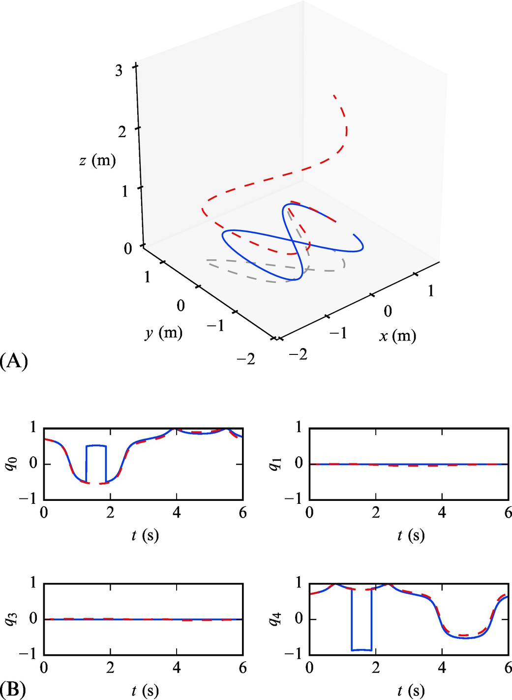
Example 5.8
Simulate measured acceleration and angular rates for a differential robot with an INS unit that drives on the curve ![]() ,
, ![]() , and z(t) = 0 (all defined in world coordinates). The time of simulation is 6 s and the sampling time is 1 ms. The INS unit is oriented so that its x-axis is tangent to trajectory, the y-axis is perpendicular to the x-axis, and the z-axis is aligned with the z-axis of the world coordinates.
, and z(t) = 0 (all defined in world coordinates). The time of simulation is 6 s and the sampling time is 1 ms. The INS unit is oriented so that its x-axis is tangent to trajectory, the y-axis is perpendicular to the x-axis, and the z-axis is aligned with the z-axis of the world coordinates.
From the measurements, estimate, the INS unit position and orientation in world coordinates. Additionally, consider sensor bias and noise and observe how this influences the estimated INS pose.
Solution
The INS unit angular rates in the simulation are obtained considering relation (5.46) to obtain the matrix of angular rates ![]() . The simulated accelerometer and gyroscope measurements are modeled using Eqs. (5.60), (5.61) and are shown in Fig. 5.7.
. The simulated accelerometer and gyroscope measurements are modeled using Eqs. (5.60), (5.61) and are shown in Fig. 5.7.
The estimated position and orientation of INS in an ideal case with no noise and bias are shown in Fig. 5.8.

The estimated pose in the case of noisy measurements and included bias are shown in Fig. 5.9, where fast growth of the position error can be observed.
A script to simulate the INS unit and estimate its pose is given in Listing 5.5 (functions rotX, rotY, and rotZ are Matlab implementations of Eqs. 5.3, 5.4, 5.5, respectively).
5.3.2 Heading Measurement
Heading measurement systems provide information about the vehicle orientation (or attitude) in space, the direction the vehicle is pointing. Several sensors can be used to estimate heading information such as a magnetometer, gyroscope, and accelerometer. Their information is integrated in sensor systems to estimate heading information (e.g., attitude, compass, or inclinometer).
The magnetometer and accelerometer provide absolute measurements of 3D direction vectors of Earth’s magnetic field (strength and direction) and Earth’s gravity direction vector (if the sensor unit is not accelerating), respectively. To lower heading estimation noise and improve accuracy also the relative measurements from the gyroscope are included in estimation filters.
To estimate orientation of the sensor unit according to some reference frame (e.g., Earth’s fixed coordinates) at least two directional vectors are required. To illustrate the idea the first sensor can be a magnetometer whose measurement model reads
where bm is the measured magnetic field in sensor coordinates, btrue is Earth’s magnetic field in Earth coordinates for some place on Earth, and rotation matrices are defined as in Eq. (5.60). btrue can be approximated as constant for some small area on Earth (e.g., 10 × 10 km2). The second sensor is the accelerometer with a model given in Eq. (5.60), whose measurement in the case of nonaccelerating motion points in the direction of gravity and the defined z-axis of Earth’s fixed coordinates.
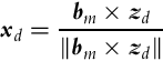
Orientation of the sensor unit according to Earth’s fixed coordinates is described by the DCM ![]() . This can be obtained by creating a matrix of the Earth’s coordinate axis vectors expressed in the local coordinates as follows. In static case accelerometer measures the direction vector from Earth’s center to the INS position. This direction therefore defines the z-axis of Earth coordinates and is expressed in a local (sensor) frame as follows:
. This can be obtained by creating a matrix of the Earth’s coordinate axis vectors expressed in the local coordinates as follows. In static case accelerometer measures the direction vector from Earth’s center to the INS position. This direction therefore defines the z-axis of Earth coordinates and is expressed in a local (sensor) frame as follows:

The direction of Earth axis x expressed in local coordinates is defined by the component of the magnetometer vector that is perpendicular to zd:
where × denotes the cross product. Direction to the north defines Earth’s y-axis expressed in local coordinates:
The obtained rotation matrix is
from where the DCM between the world and Earth coordinates is ![]() . This orientation can also be described by quaternions using relations (5.19)–(5.22) or by Euler angles using relation (5.6).
. This orientation can also be described by quaternions using relations (5.19)–(5.22) or by Euler angles using relation (5.6).
Accurate orientation estimation of the vehicle is important also when performing odometry or inertial navigation to lower orientation error and consequentially the error in position estimates. Therefore, absolute heading measurements are often combined with dead reckoning as a correction measurement in the correction step of estimators (e.g., Kalman filter).
5.3.3 Active Markers and Global Position Measurement
Localization in the environment is possible also by observing markers located at known positions in the environment. These markers can be natural if they are already part of the environment (e.g., lights on the ceiling, Wi-Fi transmitters, etc.) or they can be artificial if they are placed in the environment for the purpose of localization (e.g., radiofrequency transmitters, ultrasonic or infrared transmitters (beacons), wires buried in the ground for robotic lawn mowers, GNSS satellites, etc.).
The main advantages of using active markers are simplicity, robustness, and fast localization. However, their operational cost, maintenance, and setup cost are relatively high.
To estimate the position or pose of the system usually the triangulation or trilateration approach is applied. Trilateration uses measured distances from more transmitters to estimate the position of the receiver (mounted on the vehicle). A very well-known trilateration approach is global positioning using a global navigation satellite system (GNSS) where active markers are GNSS satellites at known locations in space. Triangulation uses measured angles to three or more markers (e.g., light source) on known locations.
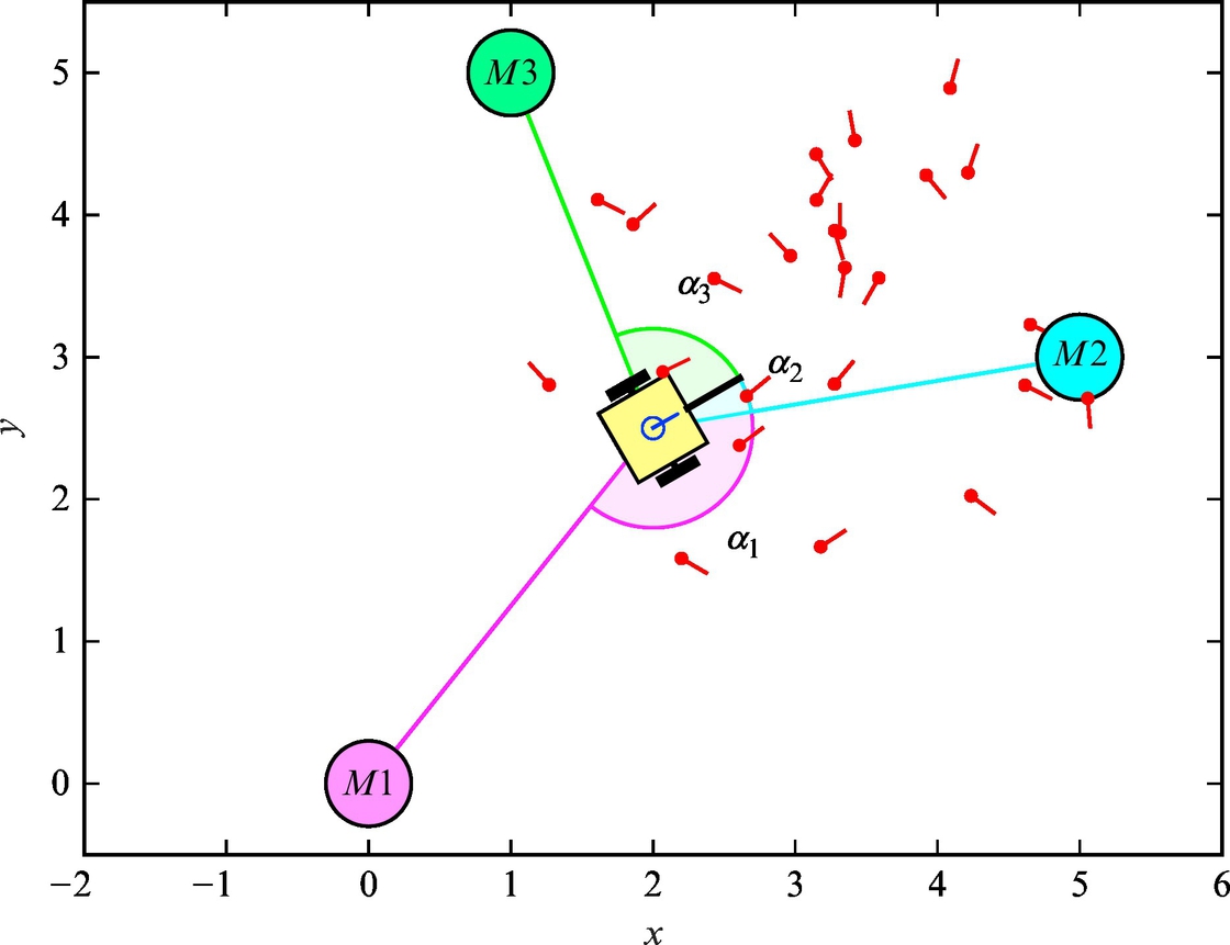
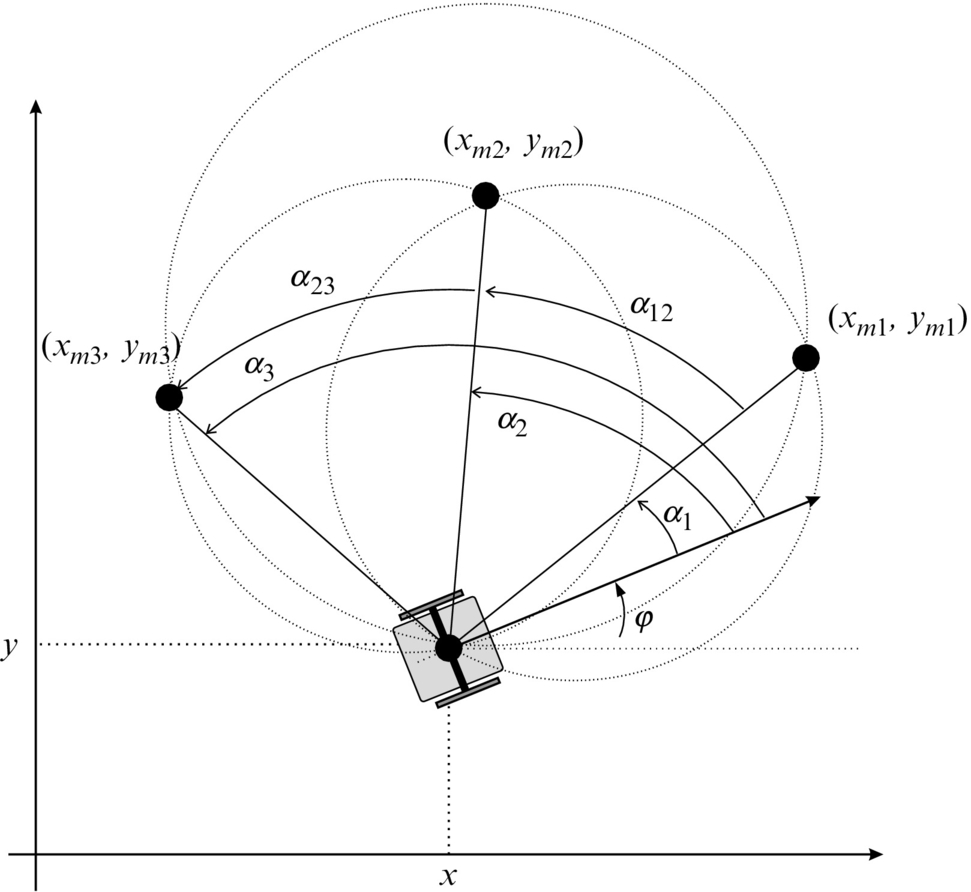
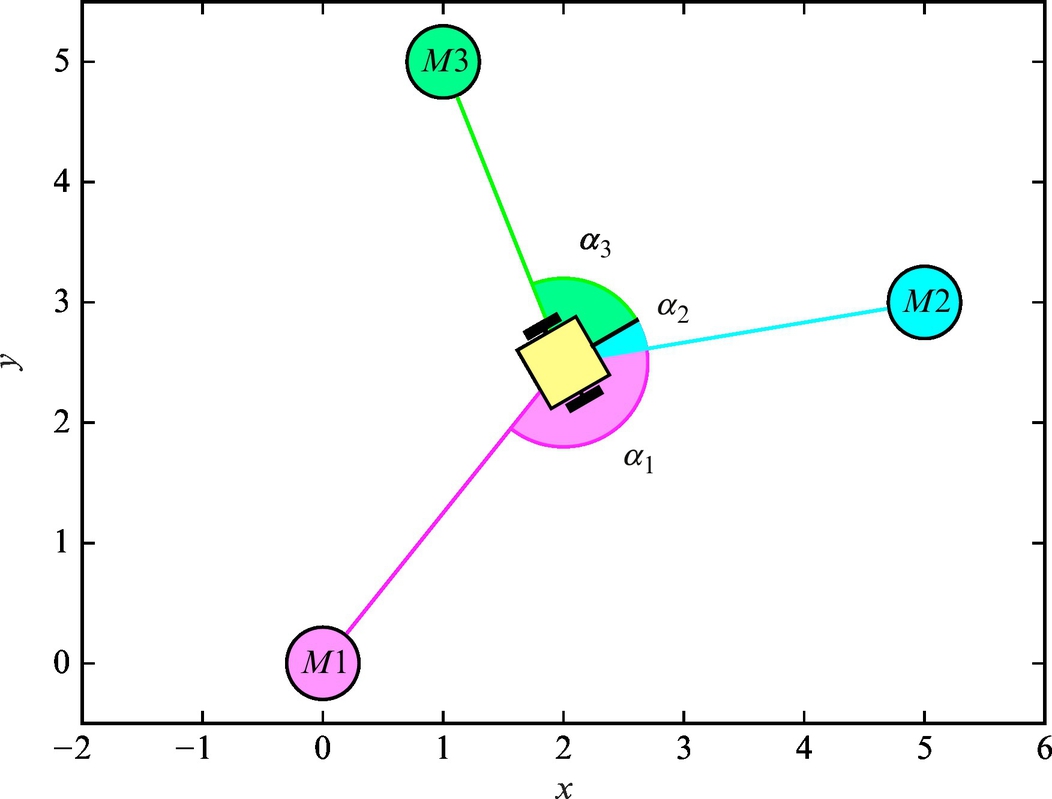
The basic idea of triangulation is illustrated in Fig. 5.10, where the robot measures relative angles αi to the active markers. Suppose there are three markers as in Fig. 5.10, the current robot pose q = [x, y, φ]T and measured angles αj (j = 1, 2, 3) are related by the following relations:
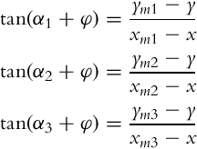
To obtain the triangulation problem solution relations in Eq. (5.69) need to be solved for q = [x, y, φ]T.

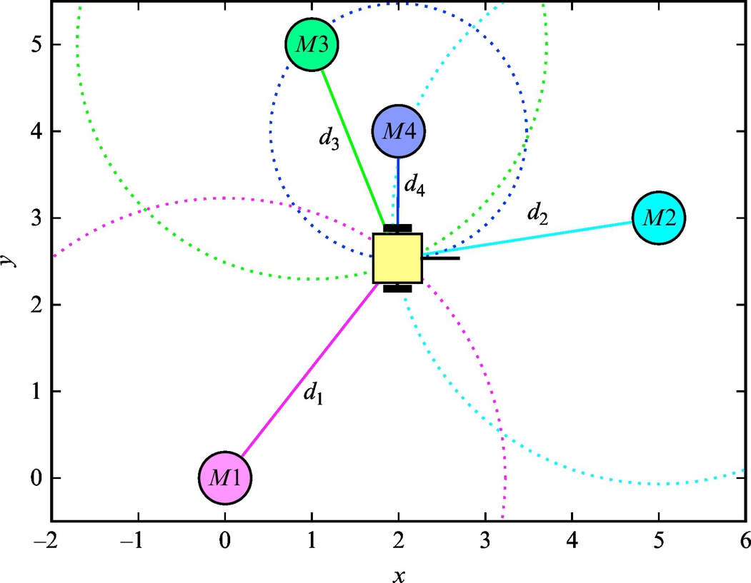
The basic idea of trilateration is illustrated in Fig. 5.14, where the current robot position, measured distances to markers, and their positions are related by the following set of equations:
In the following some examples of trilateration and triangulation are illustrated.
Example 5.9
The robot is equipped with sensor which can measure direction to the active markers. There are three active markers placed at known locations m1 = [xm1, ym1]T = [0, 0]T, m2 = [xm2, ym2]T = [5, 3]T, and m3 = [xm3, ym3]T = [1, 5]T. At a current robot pose q = [x, y, φ]T measured directions are given as a relative angles α1 = −2.7691, α2 = −0.3585, and α3 = 1.4277.
What is the current robot pose q?
There are many possible solutions to solve this triangulation problem, and here two possibilities are shown. In the first part of the solution, particle swarm optimization (PSO) is applied. Some more details about PSO can be found in Section 3.3.9. In the second part of the solution a popular geometric algorithm based on the intersection of circular arcs is used.
The current robot pose q = [x, y, φ]T and measured angles αj (j = 1, 2, 3) are related by the relations in Eq. (5.69). The task of the PSO algorithm is to find unknowns (x, y, and φ) so that the relations in Eq. (5.69) are valid. Each particle position presents one candidate solution (qi) and during optimizations a swarm of particles updates toward more optimal solutions. The criteria for optimality of the ith particle solution is given as follows:
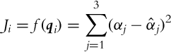
where ![]() is the simulated measurement of the ith particle that is obtained from Eq. (5.69):
is the simulated measurement of the ith particle that is obtained from Eq. (5.69):
Note that the ![]() function must return a correct angle in range (−π, π] (in Matlab function atan2 should be used).
function must return a correct angle in range (−π, π] (in Matlab function atan2 should be used).
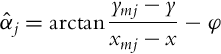
The correct solution is q = [2, 2.5, π/6]T, and the solution script is given in Listing 5.6 and the resulting situation is shown in Fig. 5.11.
Among many analytical solutions for the triangulation problem, the most often used one computes the intersection of circular arcs. Here the basic idea is described and only the final analytical solution is used to compute robot pose. The complete derivation of the algorithm can be found in [3].
The algorithm is based on three circles where each circle is defined by three points: any pair of markers mi, mj, (i, j = 1, 2, 3, i≠j), and robot position x, y (see Fig. 5.12).
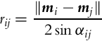
The robot position and the two markers are connected by two lines with the angle between the lines αij = αj − αi. The centers and radius of those three circles are

Because α13 = α12 + α33 only two of those angles are independent and the two belonging circles (for α12 and α23) are
The intersection of both circles (Eq. 5.73) is the solution for the robot position. For more details on how to obtain the analytical solution see [3]. Here, only the final solution is stated. A new temporary coordinate frame is defined so that m2 is in its origin and m3 lies on its x-axis. With these temporary coordinates the solution is easier to find. The rotation matrix from reference to temporary coordinates reads

where ![]() . Markers expressed in temporary coordinates (
. Markers expressed in temporary coordinates (![]() ) are obtained by transformation
) are obtained by transformation ![]() . The intersection of the circles in temporal coordinates (
. The intersection of the circles in temporal coordinates (![]() ,
, ![]() ) reads
) reads

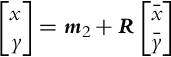
where ![]() . The solution in the reference coordinates is
. The solution in the reference coordinates is
and orientation of the robot is
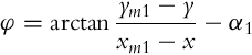
A complete algorithm to obtain the solution is given in Matlab Listing 5.7. The solution is shown graphically in Fig. 5.13.
Example 5.10
The robot is equipped with a sensor that can measure the distance to the active markers. This can be done by measuring the traveling time of the signal from the marker (transmitter) to the robot with the receiver.
There are three active markers placed at known locations: m1 = [xm1, ym1]T = [0, 0]T, m2 = [xm2, ym2]T = [5, 3]T, and m3 = [xm3, ym3]T = [1, 5]T.
At a current robot position r = [x, y]T measured distances are d1 = 3.2016 m, d2 = 3.0414 m, and d3 = 2.6926 m as illustrated in Fig. 5.14.

What is the current robot position r?
This can again be solved by some optimization algorithm similarly as in Example 5.9 with PSO or using some analytical solution.
Solution
The task of the trilateration algorithm is to find unknown position x, y so that the relations in Eq. (5.70) are valid. This can be done with PSO similarly as in Example 5.9, where the implementation needs to be modified to include relations (5.70) in computation of the criteria function.
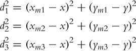
The solution of Eq. (5.70) can also be done analytically. Many different algorithms can be implemented; here, a simple solution is given. Subtracting the third equation in Eq. (5.70) from the first and the second one results in

By rearranging
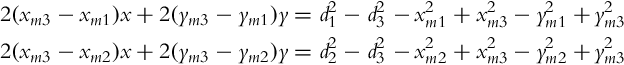
we obtain linear equations in terms of x and y, which can be written in matrix A r = b where

and

from where an unknown position is obtained:
The correct solution is r = [2, 2.5]T, and Matlab script implementation is given in Listing 5.8.
Example 5.11
In Example 5.10 measured distances were exact, which is an unrealistic assumption. Measurements are normally corrupted with noise and other disturbances; therefore, an overdetermined system with more than three markers is needed to minimize error in the position estimate. To illustrate this use n = 4 markers at locations m1 = [xm1, ym1]T = [0, 0]T, m2 = [xm2, ym2]T = [5, 3]T, m3 = [xm3, ym3]T = [1, 5]T, and m4 = [xm4, ym4]T = [2, 4]T. And measured distances corrupted with noise are d1 = 3.2297 m, d2 = 3.0697 m, d3 = 2.7060 m, and d4 = 1.4759 m. Estimate the current robot position r.
Solution
The solution that minimize mean-square error ∥A r −b∥ of an overdetermined system with n active markers is obtained as follows. Matrix A becomes

and

Finally using pseudo inverse the solution is obtained:
For given distances the solution is r = [1.9873, 2.5337]T and the Matlab script implementation is given in Listing 5.9. The solution is also shown in Fig. 5.15.
Global Navigation Satellite System
The most often used localization system using the trilateration principle is the Global Navigation Satellite System (GNSS). Satellites present active markers that transmit coded signals to the GNSS receiver station whose position needs to be estimated by trilateration. Satellites have very accurate atomic clocks and their positions are known (computed using Kepler elements and other TLE [two-line element set] parameters). There are several GNSS systems: Navstar GPS from ZDA, Glonass from Russia, and Galileo from Europe. The Navstar GPS system is designed to operate with at least 24 satellites that encircle Earth twice a day at a height of 20,200 km.
GNSS seems to be a very convenient sensor system for localization but it has some limitations that need to be considered when designing mobile systems. Its use is not possible where obstacles (e.g., trees, hills, buildings, indoors, etc.) can block the GNSS signal. Multiple signal reflections lead to multipath problems (wrong distance estimate). The expected accuracy of the system is approximately 5 m for single receiver system and approximately 1 cm for referenced systems (with additional receiver in reference station).
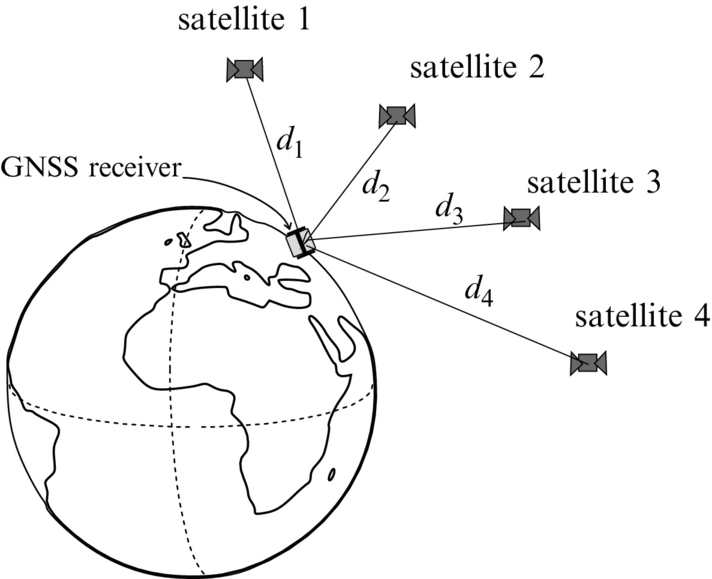
A simplified explanation of GNSS localization is as follows. GNSS receivers measure the traveling time of a GNSS signal from a certain satellite. Traveling time is the difference of the reception time tr and transmission time tt. Knowing that the signal travels at the speed of light c the distance between the receiver and satellite is computed. However, the receiver clock is not as accurate as the atomic clock on satellites. Therefore, some time bias or distance error appears, which is unknown but equal for all distances to satellites. The GNSS receiver therefore needs to estimate four parameters, namely its 3D position (x, y, and z) and time bias tb.
If around each received satellite a sphere with measured distance is drawn, the following can be concluded. The intersection of two spheres is a circle and the intersection of three spheres are two points where the receiver can be located. Therefore, we need at least four spheres to reliably estimate the position of the receiver. If the receiver is on the Earth’s surface then Earth can be considered as the fourth sphere to isolate a correct point obtained from the intersection of three satellite’ spheres. Ideally only three satellite receptions would be enough. But as already mentioned the receiver clock is inaccurate and this causes unknown time bias tb. The intersection of the four spheres (three from satellites and the fourth from Earth) is therefore not a point but an area. To estimate tb and lower localization error also the reception of the fourth satellite is required. Therefore, a minimum of four satellite receptions is required for GNSS localization as shown in Fig. 5.16. GNSS localization therefore is needed to solve the following set of equations:
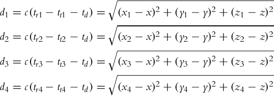
where unknowns are the receiver position x, y, z and the receiver time drift td. For ith satellite the known values are position (xi, yi, zi), reception time tri and transmission time tti, and speed of light c.
5.3.4 Navigation Using Environmental Features
Features are a subset of patterns that can be robustly extracted from raw sensor measurements or other data. Some examples of features are lines, line segments, circles, blobs, edges, corners, and other patterns. Among other applications, features detected in the environment can be utilized for the purpose of mobile robot pose estimation (localization) and map building. For example, in the case of a 2D laser range scanner the obtained range (distance and angle) data can be processed to extract line segments (features). Line features in the local coordinate frame of the mobile robot can then be compared to the global map of the environment, which is also represented with a set of lines, in order to determine the mobile robot pose in the map. Nowadays, among the various sensors used in mobile robotics, the camera as a sensor is gaining more and more attention. Over the recent years many machine vision algorithms have been developed that enable detection of image features, which can also be used for measurement of a robot pose in the environment. Approaches that are based on features normally include the following steps: feature extraction, feature description, and feature matching. In the phase of feature extraction, raw data are processed in order to determine feature locations. The neighboring area around the detected feature location is normally used in order to describe the feature. Feature descriptors can then be used in order to find similar features in the process of feature matching.
Features are located at known locations. Therefore, their observation can improve knowledge about mobile robot location (lower location uncertainty). The list of features with their locations is called a map. This requires either an offline learning phase to construct a map of features or online localization and map building (simultaneous localization and mapping [SLAM]). The former approach is methodologically simpler but impractical in practice especially for larger environments. It requires the use of some reference localization system to map observed features, or this must be done manually. The latter approach builds a map simultaneously while localizing, and the main idea is to localize from observed features that are already in the map and storing newly observed features based on localized location. For reliable feature detection and robot localization usually as accurate as possible, dead reckoning is preferred. In case features are non or weakly separable (e.g., tree trunks in an orchard or detection of straight-line segments in buildings) the approximate information about the robot’s location is needed to identify the observed features.
An approximate location of the robot in current time is obtained from the location at a previous time and dead reckoning prediction of relative motion from a previous location to the current one.
Features are said to be natural if they are already part of the environment, and they are artificial if they are made especially for localization purposes. Examples of natural features in structured environments (typically indoor) are walls, floor pates, lights, corners, and similar features, while in the nonstructured environments (usually outdoor) examples of features are three trunks, road signs, etc. Artificial features are made solely for the purpose of localization to be easily and robustly recognized (color patches, bar codes, lines on the floor, etc.).
Usually obtaining features requires some processing over raw sensor data in order to obtain more compact, more informative, and abstract presentation of the current sensor view (line presentation vs set of points). In some cases also a raw sensor measurement (LRF scan or camera image) can be used for the localization process by correlating the sensor view with a stored map.
Very often can visual features be detected with some image sensors. One of the simplest and most used features are straight lines. They can be detected in the environment by a camera or a laser range scanner (LRF).
Straight-Line Features
The use of straight lines as features in localization is a very common choice as they are the simplest geometric features. Straight-line features can be used to describe indoor or outdoor environments (walls, flat objects, road lines, etc.). By comparing currently observed feature parameters and the parameters of a priori known environment map the robot pose can be estimated.
A very popular sensor for this purpose is the LRF, which measures the cloud of reflection points in the environment. From this measured cloud of points (usually 2D) straight-line parameters are estimated using one of several line-extraction algorithms. The line fitting process usually requires two steps: the first one is identification of clusters that can be presented by a line, and the second is estimation of line fitting parameters for each cluster using the least squares method or something similar. Usually these two steps are performed iteratively.
Split-and-Merge Algorithm
A very popular algorithm for LRF data is the split-and-merge algorithm [4, 5], which is simple for realization and has low computational complexity and good performance. Its main operation is as follows. The algorithm requires batched data that is iteratively split to clusters where each cluster is described by a linear prototype (straight line for 2D data). The algorithm can only be applied to sorted data where consecutive data samples belong to the same straight line (data from LRF are sorted).
Initially all data samples belong to one cluster whose linear prototype (straight-line) parameters are identified. The initial cluster is then split in two new clusters at the sample which has the highest distance from the initial prototype if this distance is higher than the threshold dsplit. The choice of dsplit depends on data noise and must be selected higher than the expected measurement error due to the noise (e.g., three standard deviations). When clustering is finished collinear clusters are merged. This step is optional and is usually not needed in sorted data streams.
For each cluster j (j = 1, …, m) the linear prototype is defined in normal form:
where z(k) = [x(k), y(k)]T is the kth sample (k = 1, …, n and n is the number of all samples) which lies on the straight line defined by parameters θ. For cluster j, which contains samples kj = 1, …, nj the parameter vector θj can be estimated using singular value decomposition as follows. The regression matrix,
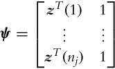
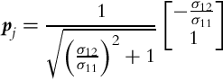
defines a set of homogenous equations in matrix form ψ θj = 0, where the prototype parameters θj need to be estimated in the sense of a least-squares minimization. The solution presents the eigenvector (pr = [px, py, pp]T) of the regression matrix ψTψ belonging to the minimum eigenvalue (calculated using singular value decomposition). The normal-form parameters of the prototype are obtained by normalization of pr:
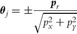
where the sign is selected opposite to the third parameter of pr (pp). For data sample z(k) that is not on the prototype j the orthogonal distance is calculated by
In the case of 2D data the linear prototype can alternatively be estimated simply by connecting the first and the last data sample in the cluster. This, however, is not optimal in a least squares sense but it lowers the computational complexity and ensures that the sample that defines the split does not appear at the first or the last data sample.
An example of fitting raw LRF data to straight lines is given in Example 5.12.
Example 5.12
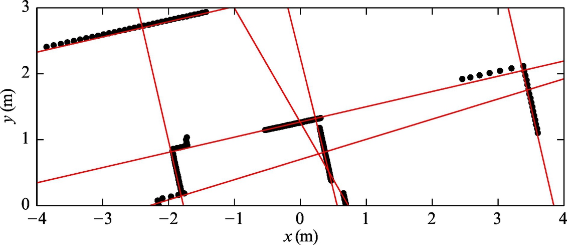
For raw laser range scanner data consisting of 180 reflection points (see Fig. 5.17 and Listing 5.10) estimate straight-line clusters that best describe the scan. Clustering is done using distance threshold dsplit = 0.06 m.

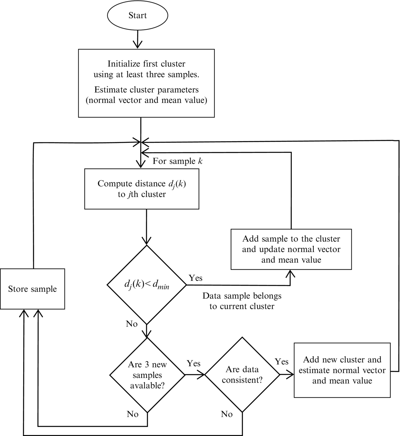
Evolving Straight-Line Clustering
Similarly as in split-and-merge clustering, straight lines can also be estimated in the case of streamed data. Clustering is done online and is iteratively updated when new data arrives. An example of a simple and computationally efficient algorithm is the evolving principal component clustering [6]. A brief description of its main steps are as follows.
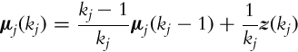
The jth prototype that models the data z(kj) (kj = 1, …, nj) in the cluster j is as follows:
where μj(kj) is the mean value of the data in cluster j that updates in each iteration (when new sample is available) by
and pj is the normal vector of the jth prototype. It is computed from the jth cluster covariance matrix (for 2D data),
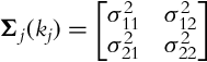
as follows:
The covariance matrix is updated iteratively using

The current sample, z(k), needs to be classified in one of the existing prototypes j (j ∈{1, …, m}). This is done by calculating the orthogonal distance dj(k) from each jth prototype:
If dj(k) = 0 the data sample lies on the linear prototype j. The sample belongs to the jth cluster if dj(k) for the jth cluster is the smallest and less than the predefined threshold distance dmin (dj(k) < dmin). In [6] robust clustering is proposed, where dmin is estimated online from the jth cluster data.
The basic idea of the clustering algorithm is illustrated in Fig. 5.18. It can be applied online to sorted data arriving from some stream or to a batched data sample (as split-and-merge). Classification results of Example 5.12 would, at a similar clustering quality as the split-and-merge algorithm, require less computational effort.
Example 5.13
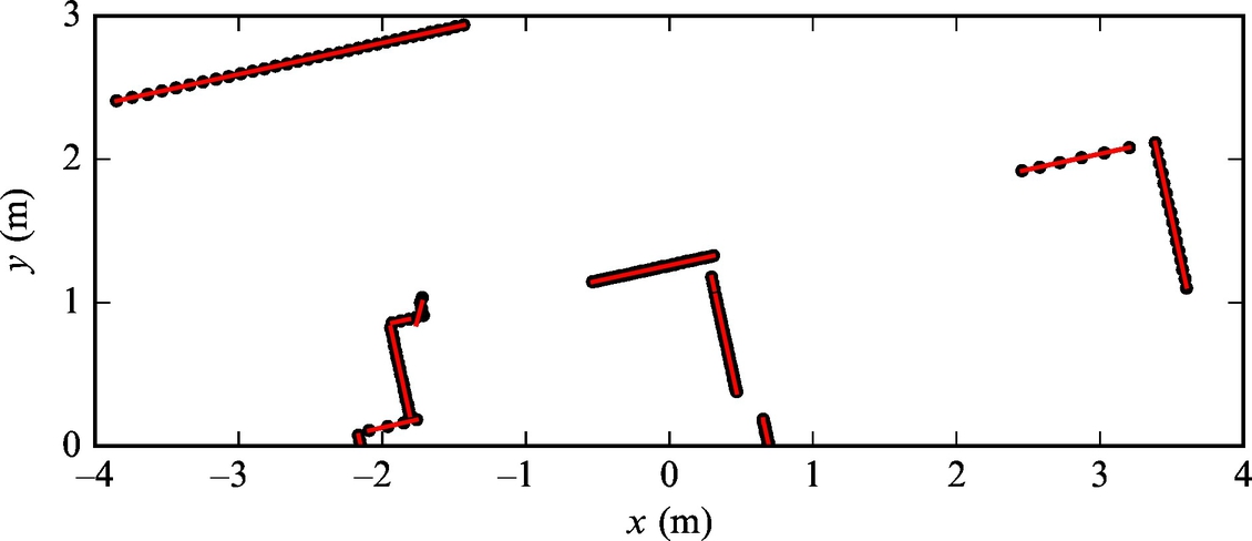
For raw laser range scanner data consisting of 180 reflection points (see Fig. 5.17 and the beginning of the solution for points coordinates) estimate straight-line clusters that best describes the scan. Clustering is done using the evolving straight-line clustering algorithm.
Solution
The current sample belongs to jth cluster if its distance dj(k) to the cluster’s line is smaller than the threshold dmin (dj(k) < dmin). dmin can be a constant or as in this example estimated online. The threshold distance parameter dmin is computed from the estimated cluster distance variance σj(kj) (distance variance of samples from the line). The variance recursive estimate reads ![]() and the threshold is
and the threshold is ![]() , where κmax = 7 is the tuning parameter.
, where κmax = 7 is the tuning parameter.
Implementation of line estimation is given in Listing 5.12 (laser scan data is defined in Listing 5.10). Estimated line segments are shown in Fig. 5.19.
Hough Transform
The Hough transform [7] is a very powerful approach to estimating geometric primitives mostly used in image processing. The incoming data are transformed in the parameter space (e.g., straight-line parameters), and by locating the maxima the number and the parameters of the lines are obtained.
The algorithm requires quantization of parameter space. Fine quantization increases accuracy but requires quite some computational effort and storage. Several studies proposed methods to avoid quantization and increase accuracy of Hough transform, such as randomized Hough transform or adaptive implementations, as reported in [8, 9].
The Hough transform can reliably estimate the clusters in the presence of outliers. In its basic version the straight-line parameters α and d are defined by the linear prototype (5.82), where ![]() . The normal line parameters’ ranges − π < α ≤ π and dmin < d ≤ dmax are presented in the accumulator by quantization to N discrete values for α and M discrete values for d.
. The normal line parameters’ ranges − π < α ≤ π and dmin < d ≤ dmax are presented in the accumulator by quantization to N discrete values for α and M discrete values for d.
For each data sample x(k), y(k) and all possible values for ![]() where n ∈{1, …, N}) solutions for parameter d(n) are computed. Each pair α(n), d(n) presents a possible straight line containing sample x(k), y(k). A corresponding location in the accumulator is increased by 1 for each computed parameter. When all data samples are processed the cells of the accumulator with the highest values are identified straight-line clusters. Some a priori knowledge is therefore required to properly select quantization of the parameter space and the threshold value to locate the maximum in the accumulator.
where n ∈{1, …, N}) solutions for parameter d(n) are computed. Each pair α(n), d(n) presents a possible straight line containing sample x(k), y(k). A corresponding location in the accumulator is increased by 1 for each computed parameter. When all data samples are processed the cells of the accumulator with the highest values are identified straight-line clusters. Some a priori knowledge is therefore required to properly select quantization of the parameter space and the threshold value to locate the maximum in the accumulator.
Example 5.14
For raw laser range scanner data consisting of 180 reflection points (see Fig. 5.21 and the beginning of the solution for point coordinates) estimate straight-line clusters that best describe the scan. Clustering is done using the Hough transform where normal straight-line parameters α and d are quantized to 720 discrete values.
Solution
A possible solution in Matlab script is given in Listing 5.13 (laser scan data is defined in Listing 5.10) where the function houghpeaks is used to find maximums in the accumulator. The obtained accumulator is shown in Fig. 5.20 and identified clusters in Fig. 5.21.