
Sensors Used in Mobile Systems
Abstract
Sensors are one of the key elements in mobile robotics. Together with other essential elements, they enable mobile robots to autonomously perform their actions, such as trajectory tracking, to locate and track targets, act safely by preventing collisions, and to localize and map the environment. Although they play a vital role they are also a limiting factor in mobile robotics because perfect, robust, and available sensors that would directly measure robot location are usually not available. Therefore, this chapter starts by introducing the different transformations that are later needed to relate local sensor-measured information to the information in robot coordinates. Then the main methods and sensors used to estimate robot pose are presented. They need to be a part of every robot localization system. The chapter ends with brief overview of sensors, their classifications, and main characteristics.
Keywords
Sensors; Pose estimation; Transformations; Dead reckoning; Active markers; Features
5.1 Introduction
Wheeled mobile robots need to sense the environment using sensors in order to autonomously perform their mission. Sensors are used to cope with uncertainties and disturbances that are always present in the environment and in all robot subsystems. Mobile robots do not have exact knowledge of the environment, and they also have imperfect knowledge about their motion models (uncertainty of the map, unknown motion models, unknown dynamics, etc.). The outcomes of the actions are also uncertain due to nonideal actuators. The main purpose of the sensors is therefore to lower these uncertainties and to enable estimation of robot states as well as the states of the environment.
Usually there is no elegant single sensor solution (especially for indoor use) that would be accurate enough and robust in measuring desired information such as the robot pose. The pose is necessary to localize the robot, which is one of the most important challenges in mobile robotics. The developers therefore need to rely on more sensors and on a fusion of their measured information. Such approaches benefit in higher quality and more robust information. Robot pose estimation usually combines relative sensors and absolute sensors. Relative sensors provide information that is given relatively to the robot coordinates, while the information of absolute sensors is defined in some global coordinate system (e.g., Earth coordinates).
Using sensors, a mobile robot can sense the states of the environment. The measured sensor information needs to be analyzed and interpreted adequately. In the real world measurements are changing dynamically (e.g., change of illumination and different sound or light absorption on surfaces). The measurement error is often modeled statistically by a probability density function for which symmetric distribution is usually supposed or even normal distribution. However, this assumption may not always be correct (e.g., ultrasonic sensor distance measurement can be larger than the true distance due to multiple reflections of the ultrasound path from the sensor transmitter to the sensor receiver).
First, the coordinate system transformations are briefly described. They are needed to correctly map sensor measurements to the robot and to estimate relevant information in robot-related coordinates. Then, the main localization methods for estimation of robot pose in the environment using specific sensors are explained. Finally, a short overview of sensors used in mobile robotics is given.
5.2 Coordinate Frame Transformations
Sensors that are mounted on the robot are usually not in the robot’s center or in the origin of the robot’s coordinate frame. Their position and orientation on the robot is described by a translation vector and rotation according to the robot’s frame. Those transformations are needed to relate measured quantities in the sensor frame to robot coordinates.
With these transformations we can describe how the sensed direction vector (e.g., accelerometer, magnetometer) or sensed position coordinates (e.g., laser range scanner or camera) are expressed in the robot coordinates. Furthermore, mobile robots are moving in space, and therefore, their poses or movements can be described by appropriate transformations.
Here, a short general overview for 3D space is given, although in wheeled mobile robots two dimensions are usually sufficient (e.g., motion on the plane described by two translations and one rotation). First some notations for rotation transformation will be described, and later a translation will be included.
5.2.1 Orientation and Rotation
Orientation of some local reference frame (e.g., sensor) according to the reference frame (e.g., robot) is described by a rotation matrix R:
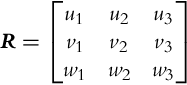
where unit vectors of a local coordinate system u, v, and w are expressed in the reference frame by u = [u1, u2, u3]T, v = [v1, v2, v3]T, w = [w1, w2, w3]T, where u ×v = w. The rows of R are components of body unit vectors along the reference coordinate unit vectors x, y, and z. The elements of matrix R are cosine of the angles among the axis of both coordinate systems; therefore, matrix R is also called the direction cosine matrix or DCM. Because vectors u, v, and w are orthonormal the inverse of R equals to the transpose of R (![]() and R−1 =RT). The DCM has nine parameters to describe three degrees of freedom, but those parameters are not mutually independent but are defined by six constraint relations (sum of squared elements of each line in R is one and a dot product of any couple of the lines in R is zero).
and R−1 =RT). The DCM has nine parameters to describe three degrees of freedom, but those parameters are not mutually independent but are defined by six constraint relations (sum of squared elements of each line in R is one and a dot product of any couple of the lines in R is zero).
The vector in a local (body) coordinate frame vL is expressed from a global coordinate (reference) using the following transformation
Matrix ![]() therefore transforms vector description (given by its components) in the global coordinates to the vector description in the local coordinates.
therefore transforms vector description (given by its components) in the global coordinates to the vector description in the local coordinates.
Basic rotation transformations are obtained by rotation around axis x, y, and z by elementary rotation matrices:

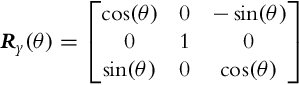

where Raxis(angle) is rotation around the axis for a given angle. Successive rotations are described by the product of the rotation matrix where the order of rotations is important. DCM is the elementary presentation of the rigid body orientation; however, in some cases other presentations are more appropriate. Therefore two additional methods will be presented in the following.
Euler Angles
Euler angles describe orientation of some rigid body by rotation around axes x, y, and z. Those angles are marked as
• φ: roll angle (around x-axis),
• θ: pitch angle (around y-axis), and
• ψ: yaw or heading angle (around z-axis).
There are 12 possible rotation combinations around axes x, y, and z [1]. The most often used is the combination 3–2–1, where the orientation of somebody coordinate frame according to the reference coordinate frame is obtained from the initial pose where both coordinate frames are aligned and then the body frame is rotated in the following order:
1. First is rotation around z-axis for yaw angle ψ,
2. then rotation around newly obtained y for a pitch angle θ, and
3. finally rotation around newly obtained x for a roll angle φ.
The DCM of this rotation transformation is

and the Euler presentation is as follows:

Parameterization using Euler angles is not redundant (three parameters for three degree of freedom). However, its main drawback is that it becomes singular at rotation θ = π/2 where rotation around z- and x-axes have the same effect (they coincide). This effect is known as Gimbal lock in classic airplane gyroscopes. In rotation simulation using Euler angles notation, this singularity appears due to division by ![]() (see Eq. 5.47 in Section 5.2.3).
(see Eq. 5.47 in Section 5.2.3).
Quaternions
Quaternions present orientation in 3D space using four parameters and one constraint equation without singularity problems such as in Euler angles presentation. Mathematically the quaternions are a noncommutative extension of the complex numbers defined by
where complex elements i, j in k are related by expression i2 =j2 =k2 = i j k = −1. q0 is the scalar part of the quaternion and q1i + q2j + q3k is termed the vector part. The quaternion norm is defined by
where q* is the conjugated quaternion obtained by q* = q0 − q1i − q2j − q3k. The inverse quaternion is calculated using its conjugate and norm value as follows:

Rotation in space is parameterized using unit quaternions by

where vector eT = [e1, e2, e3] is the unit vector of the rotation axis and Δφ rotation angle around that axis. For unit quaternion it holds ![]() .
.
Transformation
rotates vector v = [x, y, z]T expressed by quaternion
(or equivalently qv = [0, x, y, z]T) around axis e for angle Δφ to the vector v′ = [x′, y′, z′]T expressed by quaternion
where ∘ denotes the product of quaternions defined in Eqs. (5.16), (5.17).
An additional advantage of quaternions is the relatively easy combination of successive rotations. Product of two DCM can be equivalently written by the product of two quaternions [1]. Having two quaternions,
and
and rotating some vector from its initial orientation first by rotation defined by q′ and then for rotation defined by q, we obtain the following:

or in vector-matrix form

The relation between the quaternion and DCM presentation is given by

or in opposite direction
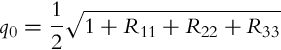


If q0 in Eq. (5.19) is close to zero then the transform from DCM to quaternion (relations 5.19–5.22) is singular. In this case we can calculate the quaternion using equivalent form (relations 5.23–5.26) without numerical problems:


where ![]()
The relation between quaternions and Euler angles (notation 3–2–1) is obtained by matrices Rx(φ), Ry(θ), and Rz(ψ), which suits to quaternions ![]() ,
, ![]() in
in ![]() . The quaternion for rotation 3–2–1 is
. The quaternion for rotation 3–2–1 is
or in vector form

The opposite transformation is


Example 5.1
A sensor (magnetometer) coordinate system is rotated according to a robot coordinate system. Lets mark the sensor coordinate system as local (L) and the robot coordinate system as global (G). The orientation of the sensor according to the robot is described by two rotations. Suppose that initially (L) is aligned to (G) then rotating (L) around x-axis for αx = 90 degree and finally around new y-axis for αy = 45 degree. Answer the following:
1. What is the orientation of the sensor expressed by the DCM (![]() ) according to robot coordinates?
) according to robot coordinates?
2. Determine Euler angles (notation 3–2–1) for this transformation.
3. Determine quaternion ![]() that describes this transformation.
that describes this transformation.
4. The magnetometer measures direction vector v = [0, 0, 1]T of the magnetic field. What is the presentation of this vector in robot coordinates?
Solution
1. Final orientation is described by the rotation matrix obtained from successive rotations where multiplication order is important.

Rows of matrix ![]() are components of the sensor axis expressed in robot coordinates, which is seen from a graphical presentation of this rotation.
are components of the sensor axis expressed in robot coordinates, which is seen from a graphical presentation of this rotation.

2. Euler angles for 3–2–1 notation are calculated from matrix ![]() :
:
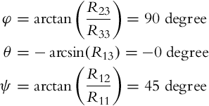
where the rotation matrix is obtained by ![]() and where elementary rotations Rx(φ), Ry(θ), and Rz(ψ) are defined in Eq. (5.5).
and where elementary rotations Rx(φ), Ry(θ), and Rz(ψ) are defined in Eq. (5.5).

3. Quaternion ![]() is obtained by the product of quaternions for successive rotations:
is obtained by the product of quaternions for successive rotations:
where qx is according to Eq. (5.10) defined by rotation angle Δφx = 90 degree around rotation axis ex = [1, 0, 0]T and qy with rotation angle Δφy = 45 degree around rotation axis ey = [0, 1, 0]T


The final quaternion (see quaternion product definition in Eq. 5.17) reads

which suits to the rotation angle ![]() degree around the rotation axis
degree around the rotation axis ![]()
4. The measured direction vector vL = [0, 0, 1]T is in robot coordinates:
where ![]() .
.
The same is obtained by quaternions where the vector after rotation is
where ![]() and
and ![]() (see Eq. 5.9). Products of quaternions are defined in Eq. (5.17). The solution is
(see Eq. 5.9). Products of quaternions are defined in Eq. (5.17). The solution is

which is vector vG = [0.7071, −0.7071, 0]T (only the vector part of quaternion is considered).
Example 5.2
Initially global coordinate frame G and local coordinate frame L are aligned; then frame L is rotated around x-axis for angle αx = 90 degree and then again around newly obtained z-axis for angle αz = 90 degree. Answer the following:
1. What is the orientation of frame L expressed by the DCM (![]() ) according to frame G?
) according to frame G?
2. Determine Euler angles (notation 3–2–1) for this transformation.
3. Determine quaternion ![]() that describes this transformation.
that describes this transformation.
4. The vector in global coordinates is vG = [0, 0, 1]T. What is the presentation of this vector in local coordinates?
Solution
1. The DCM and graphical presentation for this rotation are


2. Euler angles (3–2–1) are
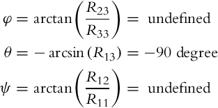
Notice that θ = −90 degree, which means that parameterization using Euler angles is singular, and therefore φ and ψ are not defined. Using Euler angles this orientation (rotation) cannot be described.
3. Quaternion ![]() is
is
where

and

which result in the rotation angle ![]() degree around axis of rotation
degree around axis of rotation ![]() .
.
4. Vector vG = [0, 0, 1]T reads in local coordinates as
or with quaternions

where the vector part is vL = [1, 0, 0]T.
5.2.2 Translation and Rotation
To make presentation more general lets mark sensor coordinates by L (as local coordinates) and robot coordinates by G (as global coordinates). Sensor location according to robot coordinates is described by translation vector ![]() and rotation matrix
and rotation matrix ![]() . Translation
. Translation ![]() describes the position of the local coordinates’ origin in global coordinates, and rotation matrix
describes the position of the local coordinates’ origin in global coordinates, and rotation matrix ![]() describes the local coordinate frame orientation according to global (robot) coordinates. A point pG given in global coordinates can be described by local coordinates using transformation
describes the local coordinate frame orientation according to global (robot) coordinates. A point pG given in global coordinates can be described by local coordinates using transformation
and its inverse transformation is given by
Example 5.3
A robot has a laser range finder (LRF) sensor that measures the position of the closest obstacle point pL = [1, 0.5, 0.4]T m in sensor coordinates. It also has a magnetometer that measures Earth’s magnetic field vector ![]() .
.
The laser range sensor is translated according to a robot (global) coordinate frame by t1 = [0.1, 0, 0.25]T and rotated (according to a robot coordinate frame) around z-axis for 30 degree. The magnetometer translation is t2 = [0, 0.1, 0.2], and rotation is described by roll, pitch, and yaw angles φ = 0 degree, θ = 10 degree, and ψ = 20 degree (Euler notation 3–2–1), respectively.
Answer the following:
1. What are the closest obstacle point coordinates in the robot coordinate system?
2. How is Earth’s magnetic field vector presented by robot coordinates?


5.2.3 Kinematics of Rotating Frames
This section will introduce how rigid body orientation presented by quaternions or the DCM is related to angular rates around local axes of the rigid body. The rigid body is rotating around its x-, y-, and z-axes with angular velocities ωx, ωy, and ωz, respectively. Therefore, the orientation of the rigid body (e.g., robot or sensor unit) is changing according to the reference coordinate system.
Rotational Kinematics Expressed by Quaternions
Time dependency of rigid body rotation (given by differential equation) can be derived from the product definition of two quaternions (5.17). If orientation q(t) of the rigid body at time t is known then its orientation in time q(t + Δt) can be written as
where Δq(t) defined the change of the rigid body orientation from q(t) to q(t + Δt). In other words Δq(t) is the orientation of the body at time t + Δt relative to its orientation at time t. The final orientation of the body q(t + Δt) is therefore obtained by first rotating the body according to some reference frame for rotation q(t), and then also for rotation Δq(t) according to q(t). Δq(t) is defined by relation (5.10)

where e(t) = [ex, ey, ez]T is the rotation axis expressed in rigid body local coordinates at time t and Δφ is the rotation angle during time period Δt. Assuming e(t) and Δφ are constant during the period Δt, the product of quaternions (5.34) can be reformulated using definition (5.17) as follows:

where I is a 4 × 4 identity matrix. For a short interval Δt we can approximate ![]() where ω(t) = [ωx, ωy, ωz]T is the vector of current angular rates, which can also be written in the form
where ω(t) = [ωx, ωy, ωz]T is the vector of current angular rates, which can also be written in the form ![]() . For small angles, Eq. (5.36) can be approximated by
. For small angles, Eq. (5.36) can be approximated by

where

A differential equation that describes rigid body orientation is obtained by limiting Δt toward zero:

where angular rates in Ω are given in the rigid body coordinates.
Rotational Kinematics Expressed by DCM
The differential equation for rigid body orientation presentation given by the DCM is derived in the following. Defining similarly as in Eq. (5.34),
where R(t) is the orientation of the rigid body at time t, R(t + Δt) is the orientation at time t + Δt, and ΔR(t) is the change of orientation (orientation of the body at time t = t + Δt) according to the orientation at time t.
Change of orientation ΔR(t) is defined as
where

and ω(t) = [ωx, ωy, ωz]T is the vector of the current angular rates of the body.
Assuming Ω′ is a constant matrix in time period Δt we can approximate ![]() . The exponent in relation (5.41) written in the Taylor series becomes
. The exponent in relation (5.41) written in the Taylor series becomes

where I is the 3 × 3 identity matrix and ![]() . For small angles σ relation (5.43) approximates to
. For small angles σ relation (5.43) approximates to
which can be used to predict rotation matrix (5.40):
The final differential equation is obtained by limiting Δt to zero:

For the sake of completeness, also the equivalent presentation of rotation parameterization using Euler angles (notation 3–2–1) is given:

where it can be seen that the notation becomes singular (the first end the third equation of Eq. (5.47) at θ = ±π/2).
5.2.4 Projective Geometry
Projection is the transformation of a space with N > 0 dimensions into a space with M < N dimensions. Normally, under a general projective transformation some information is inevitably lost. However, if multiple projections of an object are available, it is in some cases possible to reconstruct the original object in N-dimensional space. Two of the most common projective transformations are perspective projection and parallel projection (linear transformation with a focal point in infinity).
According to the pinhole camera model, the 3D point ![]() given in the camera frame C is projected to the 2D point
given in the camera frame C is projected to the 2D point ![]() in the image (picture) frame P as follows (see Fig. 5.1):
in the image (picture) frame P as follows (see Fig. 5.1):


where ![]() is the representation of the point pP in homogeneous coordinates, that is,
is the representation of the point pP in homogeneous coordinates, that is, ![]() . Matrix
. Matrix ![]() describes the internal camera model:
describes the internal camera model:

The intrinsic camera parameters contained in S are the focal length f; the scaling factors αx and αy in horizontal and vertical directions, respectively; the optical axis image center (cx, cy); and the skewness γ. The camera model parameters are normally obtained or refined in the process of camera calibration. The perspective camera model (5.48) is nonlinear because of the term ![]() (the inverse of the object distance along the z-axis in the camera frame C). Although points, lines, and general conics are invariant under perspective transformation (i.e., the points transform into points, the lines into lines, and conics into conics), the projected image is a somewhat distorted representation of reality. In general, the angles between the lines and distance ratios are not preserved (e.g., the parallel lines do not transform into parallel lines). In some particular camera configurations the perspective projection can be approximated with an appropriate linear model [2]; this can enable, for example, simple camera calibration. The camera model (5.48) can also be written as
(the inverse of the object distance along the z-axis in the camera frame C). Although points, lines, and general conics are invariant under perspective transformation (i.e., the points transform into points, the lines into lines, and conics into conics), the projected image is a somewhat distorted representation of reality. In general, the angles between the lines and distance ratios are not preserved (e.g., the parallel lines do not transform into parallel lines). In some particular camera configurations the perspective projection can be approximated with an appropriate linear model [2]; this can enable, for example, simple camera calibration. The camera model (5.48) can also be written as
The image of an object is formed on the screen behind the camera optical center (at the distance of focal length f along the negative zC semiaxis), and it is rotated for 180 degree and scaled down. When creating a visual presentation of the camera model a virtual unrotated image can be assumed to be formed in front of the camera’s optical center (on the positive zC semiaxis at the same distance from the optical center as a real image) as it is shown in Fig. 5.1.
Example 5.4
The internal camera model (5.49) has the following parameters: αxf = αyf = 1000, no skewness (γ = 0), and the image center is in the middle of the image with dimensions of 1024 × 768. Project the following set of 3D points given the camera frame to the image:
Solution
The projection of 3D points to an image according to Eq. (5.48) is given in Listing 5.1. The results are also shown graphically on the left-hand side of Fig. 5.2. Notice that the last point does not appear in the image since it is out of the image screen’s boundaries. Moreover, the fourth point also should not appear in the image since the point is behind the camera. Remember that the mathematical model (5.48) does not take visibility constraints into account. Therefore additional checks need to be made that ensure that only visible points are projected to the image: that is, the projected points must be inside the image boundaries and the point to be projected must be in front of the camera. Therefore, only the first three points actually appear in the image (see right-hand side of Fig. 5.2).


From Eq. (5.48) it is clear that every point in the 3D space is transformed to a point in 2D space, but this does not hold for the inverse transformation. Since the perspective transformation causes loss of the scene depth, the point in the image space can only be back-projected to a ray in 3D space if no additional information is available. The scene can be reconstructed if scene depth is somehow recovered. There are various techniques that enable 3D reconstruction that can be based on depth cameras, structured light, visual cues, motion, and more. The position of the point in a 3D scene can also be recovered from corresponding images of the 3D point obtained from multiple (at least two) views. Three-dimensional reconstruction is therefore possible with a stereo camera.
Multiview Geometry
Multiview geometry is not important only because it enables scene reconstruction but some of the properties can be exploited in the design of machine vision algorithms (e.g., image point matching and image-based camera pose estimation). Consider that the rotation matrix ![]() and translation vector
and translation vector ![]() describe the relative pose between two cameras (Fig. 5.3). Under the assumption that camera centers do not coincide (
describe the relative pose between two cameras (Fig. 5.3). Under the assumption that camera centers do not coincide (![]() ), the relation (5.52) can be obtained after a short mathematical manipulation (cameras with identical internal parameters are assumed):
), the relation (5.52) can be obtained after a short mathematical manipulation (cameras with identical internal parameters are assumed):


Notice that the cross product between the vectors aT = [a1a2a3] and bT = [b1b2b3] is written as a ×b = [a]×b, where [a]× is a skew-symmetric matrix:

The matrix F is known as a fundamental matrix that describes the epipolar constraint (5.52): the point ![]() is on the line
is on the line ![]() in the first image and the point
in the first image and the point ![]() lies on the line
lies on the line ![]() in the second image. Another important relation in machine vision is
in the second image. Another important relation in machine vision is ![]() , where
, where ![]() is known as the essential matrix. The relation between the essential and fundamental matrix is E =STF S.
is known as the essential matrix. The relation between the essential and fundamental matrix is E =STF S.
The epipolar constraint can be used to improve matching of image points in multiple images that belong to the same world point given the known pose between two calibrated cameras. Since the corresponding pair of the point ![]() in the first image must lie on the line
in the first image must lie on the line ![]() in the second image, the 2D searching over the entire image area is simplified to a 1D search along the epipolar line, and therefore the matching process can be sped up significantly and it can also be made more robust, since matches that do not satisfy the epipolar constraint are rejected.
in the second image, the 2D searching over the entire image area is simplified to a 1D search along the epipolar line, and therefore the matching process can be sped up significantly and it can also be made more robust, since matches that do not satisfy the epipolar constraint are rejected.
Example 5.5
A set of 3D points is observed from two cameras with relative displacement described by the rotation matrix ![]() and translation vector
and translation vector ![]() . Both cameras have the same internal camera model (5.49): αxf = αyf = 1000, no skewness (γ = 0), and image center is in the middle of the image with the dimensions of 1024 × 768. A set of projected points into the image of the first camera is
. Both cameras have the same internal camera model (5.49): αxf = αyf = 1000, no skewness (γ = 0), and image center is in the middle of the image with the dimensions of 1024 × 768. A set of projected points into the image of the first camera is
and a set of point projected into the image of the second camera is
The points in both images are shown in Fig. 5.4. Determine all possible image point correspondences taking into account the epipolar constraint. For all the matched point pairs reconstruct the position of the points in the 3D space with respect to both camera frames.

Solution
When matching points between the images from two cameras with a known relative pose between them, the points that belong to the same world point must satisfy the epipolar constraint (5.52). Eq. (5.52) has the form ![]() , that is, the homogeneous point
, that is, the homogeneous point ![]() lies on the line lT = [a b c], since ax + by + c = 0 is a line equation. Therefore, the epipolar constraint (5.52) can be utilized to find the epipolar lines
lies on the line lT = [a b c], since ax + by + c = 0 is a line equation. Therefore, the epipolar constraint (5.52) can be utilized to find the epipolar lines ![]() in the second image for every point
in the second image for every point ![]() from the first image, and vice-versa, lines
from the first image, and vice-versa, lines ![]() for every point
for every point ![]() . The epipolar lines for the first and the second image are shown in Fig. 5.5. From Figs. 5.4 and 5.5 four possible point matches can be found graphically.
. The epipolar lines for the first and the second image are shown in Fig. 5.5. From Figs. 5.4 and 5.5 four possible point matches can be found graphically.

The implementation of algorithm for point matching is given in Listing 5.2 (functions rotX and rotY are Matlab implementations of Eqs. 5.3, 5.4, respectively). The resulting point matches are collected in the index matrix pairs.
Singular Cases
The relation (5.52) becomes singular if there is no translation between the camera centers. In this case the following relation can be obtained from Eq. (5.51) if ![]() is set to zero:
is set to zero:
A similar equation form can also be obtained in a case where all the points in the 3D space are confined to a single common plane. Without loss of generality, the plane zW = 0 can be selected:
where ![]() . The transformation from the world plane to the picture plane is
. The transformation from the world plane to the picture plane is
where in this particular case ![]() . Eqs. (5.54)–(5.56) all have similar form:
. Eqs. (5.54)–(5.56) all have similar form: ![]() . The matrix H is known as homography.
. The matrix H is known as homography.
3D Reconstruction
In a stereo camera configuration the 3D position of a point can be reconstructed from both images of the point. This procedure requires finding corresponding image points among the views, which is one of the fundamental problems in machine vision. But once point correspondences have been established and the relative pose between the camera views is known (the translation between the cameras must be different from zero) and also the internal camera model is known, the 3D position of the point can be estimated. If both camera models are the same, the point depth in both camera frames (![]() and
and ![]() ) can be estimated by solving the following set of equations (e.g., using least squares method):
) can be estimated by solving the following set of equations (e.g., using least squares method):
The reconstruction problem simplifies in a canonical stereo configuration of two cameras, where one camera frame is only translated along the x-axis for baseline distance b (as shown in Fig. 5.6), since the epipolar lines are parallel and the epipolar line of the point ![]() passes through that point (not only the point
passes through that point (not only the point ![]() in the other image). In the case of a digital image, this means that the matching point of a point in the first image is in the same image row in the second image. For the sake of simplicity, set αx = αy = α and γ = 0 in the camera model (5.49). The position of a 3D world point in the first camera frame can then be obtained from two images of the world point according to
in the other image). In the case of a digital image, this means that the matching point of a point in the first image is in the same image row in the second image. For the sake of simplicity, set αx = αy = α and γ = 0 in the camera model (5.49). The position of a 3D world point in the first camera frame can then be obtained from two images of the world point according to

where the disparity was introduced as ![]() . The disparity contains information about scene depth as it can be seen from the last element in Eq. (5.58):
. The disparity contains information about scene depth as it can be seen from the last element in Eq. (5.58): ![]() . For all the points that are in front of the camera the disparity is positive, d ≥ 0.
. For all the points that are in front of the camera the disparity is positive, d ≥ 0.

Example 5.7
Assume a canonical stereo camera setup with baseline distance b = 0.2 and the following internal camera model parameters: αxf = αyf = 1000, cx = 512, and cy = 384. Reconstruct the position of a 3D point that projects to the points ![]() and
and ![]() in the first and second camera image, respectively.
in the first and second camera image, respectively.