
6.4.5 Environment Sensing
The measurement made in the environment can be used to improve the estimation of the state X (e.g., location) in this environment. Imagine that we are sleepwalking around the house in the middle of the night. When we wake up, we can figure out where we are by using our senses (sight, touch, etc.).
Mathematically, the initial knowledge about the environment can be described with probability distribution p(x) (prior). This distribution can be improved when a new measurement z (with belief p(z|x)) is available if the probability after the measurement is determined p(x|z). This can be achieved using the Bayesian rule ![]() . The probability p(z|x) represents the statistical model of the sensor, and bel(x) is state-estimate belief after the measurement is made. In the process of perception, the correction step of the Bayesian filter is evaluated.
. The probability p(z|x) represents the statistical model of the sensor, and bel(x) is state-estimate belief after the measurement is made. In the process of perception, the correction step of the Bayesian filter is evaluated.
Example 6.9
Considering Example 6.8, assume that the mobile system detects a dark cell Z = dark. The mobile system detects a dark cell with probability 0.6 and makes a mistake with probability 0.2 (detects a bright cell as dark). Hence,
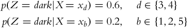
where index b indicated bright cells and index d indicated dark cells. In the beginning, the mobile system does not know its position. This can be described with a uniform probability distribution P(X = xi) = bel(xi) = 0.2, i ∈{1, …, 5}. Calculate the location probability distribution after a single measurement.
Solution
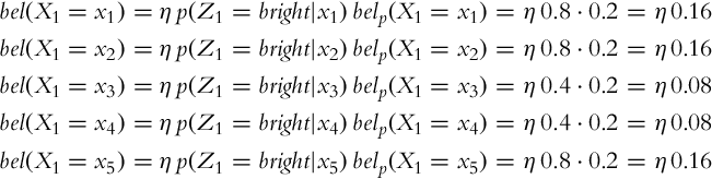
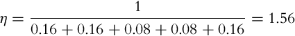
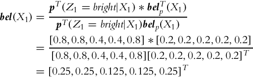
We would like to determine the distribution of conditional probability p(X1|Z = dark), the state-estimate belief after the measurement is made. The desired probability can be determined using the correction step of the Bayesian filter:
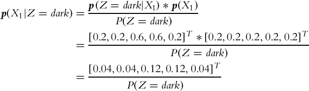
where the operator * represents the operation of element-wise multiplication of vector elements. We need to calculate the probability of detecting a dark cell P(Z = dark). Therefore the total probability must be evaluated, that is, the probability of detecting a dark cell considering all the cells:
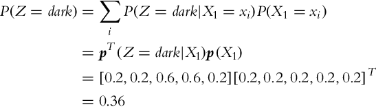
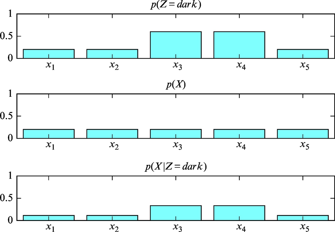
The posterior probability distribution is therefore the following:
Hence, we can conclude that the position of the mobile system is three times more likely to be in cells 3 or 4 than in the remaining three cells. The probability distributions are also shown graphically in Fig. 6.10. The solution of this example is also given in Listing 6.4.
Example 6.10
Answer the following questions about Example 6.9:
1. Can multiple measurements improve the estimated mobile system position (the mobile system does not move between the measurements)?
2. What is the probability distribution of the mobile system position if the mobile system detects a tile as dark twice in a row?
3. What is the probability distribution of the mobile system position if the mobile system detects a tile as dark and then as bright?
4. What is the probability distribution of the mobile system position if the mobile system detects a tile as dark, then as bright, and then again as dark?
Solution
1. Multiple measurements can improve the estimate about the mobile system position if the probability of the correct measurement is higher than the probability of the measurement mistake.
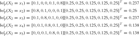
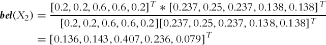
2. The probability distribution if the sensor detects cell as dark twice in a row is the following:
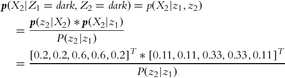
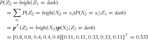
where jth element in the probability distribution p(X2|z1) is given by P(X2 = xj|z1) =pT(X2 = xj|X1)p(X1|z1) = P(X1 = xj|z1), since we have no influence on the states (see Example 6.5); we only observe the states with measurements. The conditional probability in the denominator is

Finally, the solution is

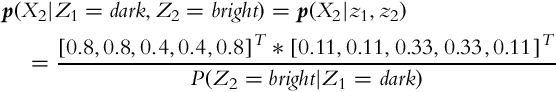
3. The bright cell is detected correctly with probability p(Z = bright|X = bright) = 1 − p(Z = dark|X = bright) = 0.8 and incorrectly with probability p(Z = bright|X = dark) = 1 − p(Z = dark|X = dark) = 0.4. The second measurement can be made based on the probability distribution p(X2|Z1 = dark):
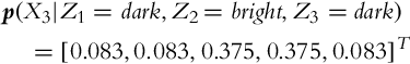
4. The state probability distribution after three measurements were made is
The implementation of the solution in Matlab is shown in Listing 6.5. The posterior state probability distributions for three time steps are presented graphically in Fig. 6.11.

6.4.6 Motion in the Environment
Mobile systems can move in the environment using some actuators (e.g., motorized wheels) and a control system. Every movement has small or large uncertainty; therefore, the movement of the mobile system through the environment increases the uncertainty about the mobile system state (pose) in the environment.
Consider that we are standing in well-known environment. We close our eyes and make several steps. After a few steps we know approximately where we are, since we know how big are our steps and we know in which direction the steps were made. Therefore, we can imagine where we are. However, the lengths of our steps are not known precisely, and also the directions of the steps are hard to estimate; therefore, our knowledge about our pose in space decreases with time as more and more steps are made.
In the case of movement without observing the states through measurement, the relation (6.28) can be reformulated:

The belief in the new state p(xk|u0:k−1) depends on the belief in the previous time step p(xk−1|u0:k−2) and conditional state transition probability p(xk|xk−1, uk−1). The probability distribution p(xk|, u0:k−1) can be determined with integration (or summation in the discrete case) of all possible state transition probabilities p(xk|xk−1, uk−1) from previous states xk−1 into state xk, given the known action uk−1.
Example 6.11
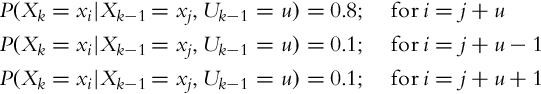
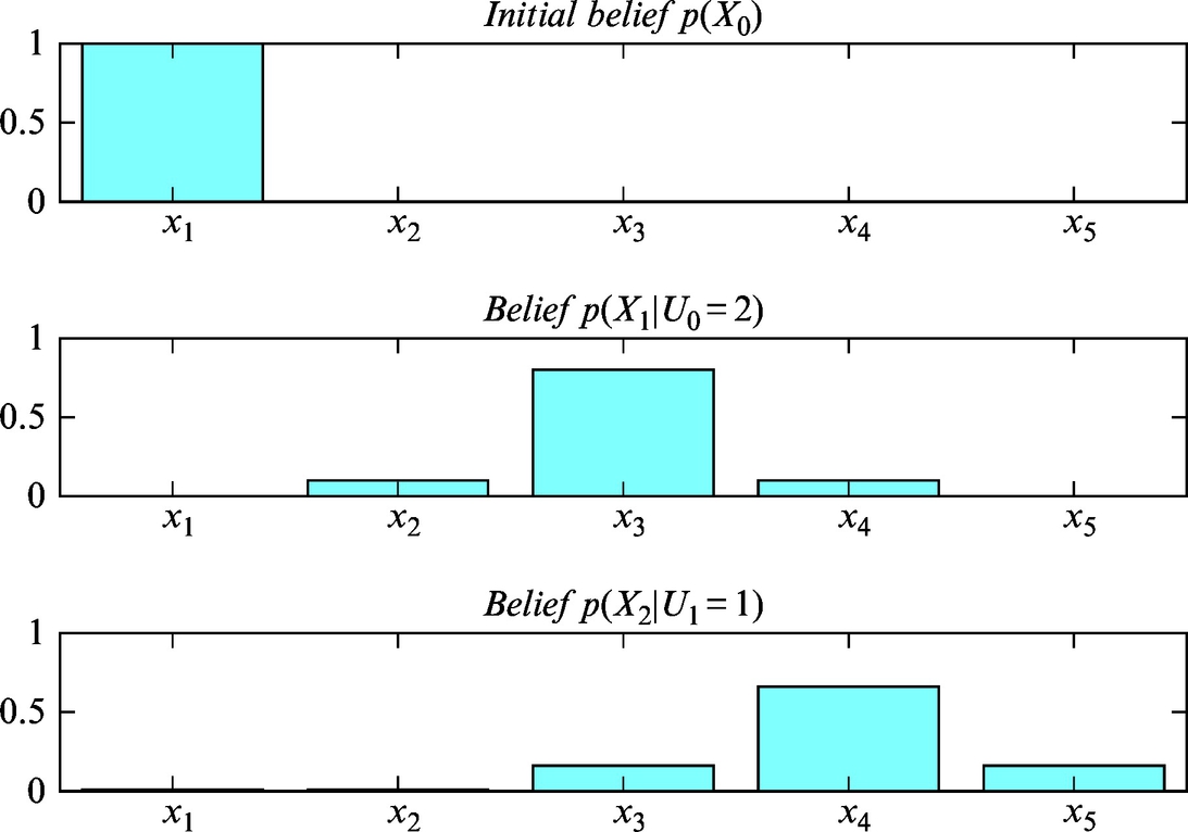
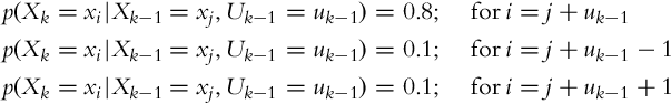
Consider again Example 6.8 and assume that the initial position of the mobile system is in the first cell (X0 = x1). The initial state can be written with probability distribution p(X0) = [1, 0, 0, 0, 0]. The mobile system can move between cells, the outcome of movement action is correct in 80%, in 10% the movement of the mobile system is one cell less than required, and in 10% the mobile system moves one cell more than required. This can be described with the following state transition probabilities:
The mobile system has to make a movement for two cells in the counter-clockwise direction (U0 = 2). Determine the mobile system position belief after the movement is made.
Solution
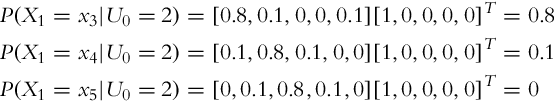
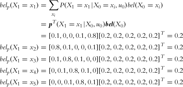
The probability distribution (belief) after the movement is made can be determined if the probabilities of the mobile system positions in every cell are calculated (total probability). The mobile system can arrive into the first cell only from cell 3 (too long move), cell 4 (correct move), and cell 5 (too short move). This yields the probability distribution of the transition into the first cell p(X1 = x1|X0, U0 = 2) = [0, 0, 0.1, 0.8, 0.1]T. After the movement the mobile system is in the first cell with probability

The probability that the mobile system after the movement is in the second cell is

Similarly, the probabilities of all the other cells can be calculated:
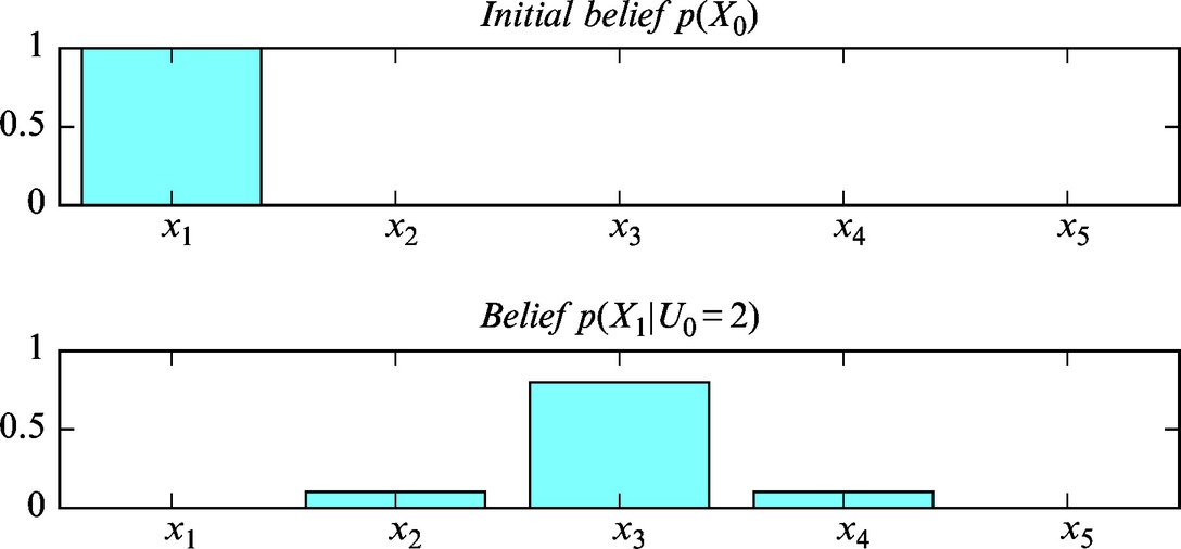
The mobile position belief after the movement is therefore
The posterior state probability distributions are presented graphically in Fig. 6.12. The implementation of the solution in Matlab is shown in Listing 6.6.
Example 6.12
What is the belief of mobile system position if after the movement made in Example 6.11 the mobile system makes another move in the counter-clockwise direction, but this time only for a single cell (U1 = 1)?
Solution
The probability distribution (belief) after the movement can again be determined if the probability that the mobile system is in a particular cell is calculated for every cell (total probability). In the case of a movement for a single cell, the first cell can be reached from cell 1 (too short move), cell 4 (too long move), and cell 5 (correct move). The mobile system can arrive to the second cell from cells 1, 2, and 5, and so on. After the movement is made, the following probabilities can be calculated:
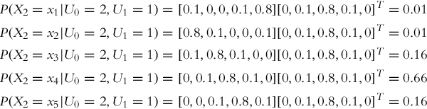
The position belief after the second movement is
and it is also shown in the bottom of Fig. 6.13. Note that the mobile system is most probably in cell 4. However, the probability distribution does not have as significant peak as it was before the second movement action was made (compare the middle with the bottom probability distribution in Fig. 6.13; the peak dropped from 80% to 66%). This observation is in accordance with the statement that every movement (action) increases the level of uncertainty about the states of the environment.
The implementation of the solution in Matlab is shown in Listing 6.7.
Example 6.13
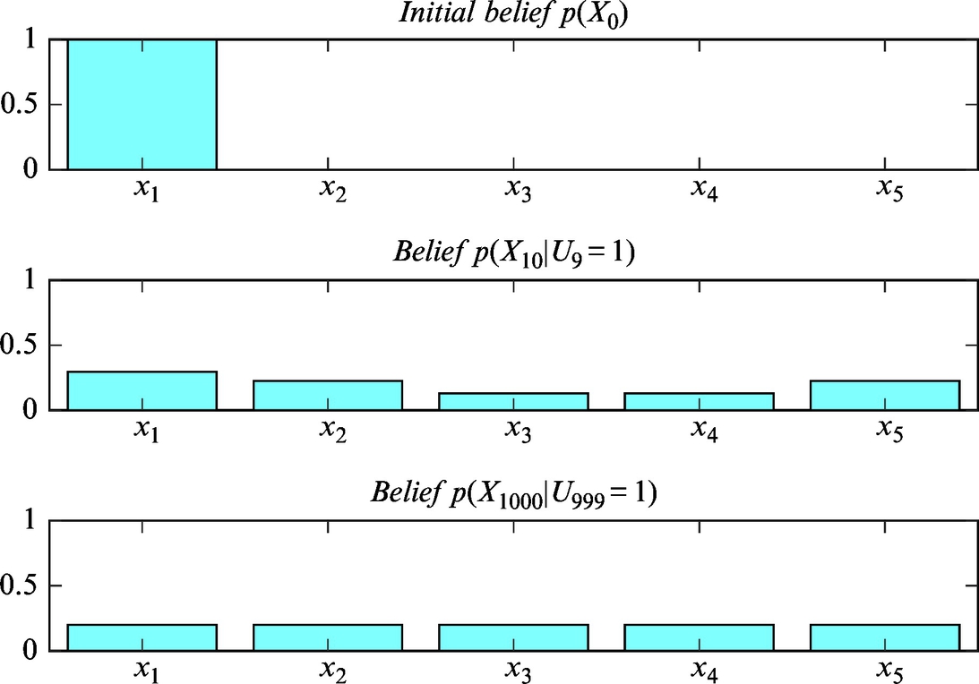
Consider that the mobile system in Example 6.11 is initially in the first cell, p(X0) = [1, 0, 0, 0, 0]. In every time step the mobile system makes one step in counter-clockwise direction.
1. What is the belief into mobile system position after 10 time steps?
2. To which value does the belief converge after an infinite number of time steps?
Solution
1. The state belief after 10 time steps is
2. After an infinite number of time steps a uniform distribution is obtained, since all the cells become equally possible to be occupied by the mobile system:
These results were also validated in Matlab (Listing 6.8) and are shown graphically in Fig. 6.14.
6.4.7 Localization in the Environment
The mobile system can estimate its location in the environment even if it does not know its initial location but has a map of the environment. The location of the mobile system can be determined precisely with probability distribution. The process of determining the location in the environment is known as localization. Localization combines the process of observation (measurement) and action (movement). As already mentioned, measurements made in the environment increase the knowledge about the location, but the movement of the mobile system through the environment decreases this information.
Localization is a process in which the mobile system repeatedly updates the probability distribution that represents the knowledge about the mobile system’s location in the environment. The peak in the probability distribution (if it exists) represents the most probable mobile system location.
The localization process is a realization of the Bayesian filter (Algorithm 3), which combines the processes of movement and perception.
Example 6.14
Consider the mobile system that moves around the environment as shown in Example 6.8. The mobile system first makes a move and then observes the environment. The initial pose of the mobile system is not known. This can be described with uniform probability distribution p(X0) = bel(X0) = [0.2, 0.2, 0.2, 0.2, 0.2].
The movement action for uk cells in the counter-clockwise direction is accurate in 80%; in 10% the movement is either a cell shorter or longer than required:
The mobile system detects a dark cell correctly with probability 0.6, and the probability of detecting a bright cell correctly is 0.8. This can be written down in mathematical form as

In every time step, the mobile system receives a command of moving for a single cell in the counter-clockwise direction (uk−1 = 1). The sequence of the first three measurements is z1:3 = [bright, dark, dark].
1. What is the belief in the first time step k = 1?
2. What is the belief in the second time step k = 2?
3. What is the belief in the third time step k = 3?
4. In which cell is the mobile system most likely after the third step?
Solution
After every movement is made a prediction step of the Bayesian filter (Algorithm 3) is evaluated, and a correction step after the measurement is made.
1. The prediction step is evaluated based on the known movement action. The small symbol xi, i ∈{1, …, 5} denotes that the location (state) of the mobile system is in cell i, and big symbol Xk denotes the vector of all possible states in time step k.
Therefore, the complete probability distribution (belief) of the prediction step is
After the measurement is obtained the correction step of the Bayesian filter is evaluated:
After considering the normalization factor,
the updated probability distribution (belief) is obtained:
The same result can be obtained from the following:
2. The procedure from the first case can be repeated again on the last result to obtain state belief in time step k = 1. First, a prediction step is repeated:
The complete probability distribution of prediction is
The correction step yields
3. Similarly as in the previous two cases, the belief distribution can be obtained for time step k = 3:

4. After the third time step, the mobile system is most likely in the fourth cell, with probability 52.8%. The second most likely cell is the third cell, with probability 24.5%.
The state beliefs for all three time steps are presented graphically in Fig. 6.15. The implementation of the solution in Matlab is shown in Listing 6.9.

6.5 Kalman Filter
Kalman filter [6] is one of the most important state estimation and prediction algorithms, which has been applied to a diverse range of applications in various engineering fields, and autonomous mobile systems are no exception. The Kalman filter is designed for state estimation of linear systems where the system signals may be corrupted by noise. The algorithm has a typical two-step structure that consists of a prediction and a correction step that are evaluated in every time step. In the prediction step, the latest system state along with state uncertainties are predicted. Once a new measurement is available, the correction step is evaluated where the stochastic measurement is joined with the predicted state estimate as a weighted average, in a way that less uncertain values are given a greater weight. The algorithm is recursive and allows an online estimation of the current system state taking into account system and measurement uncertainties.
A classical Kalman filter assumes normally distributed noises, that is, the probability distribution of noise is a Gaussian function:
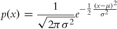
where μ is the mean value (mathematical expectation) and σ2 is the variance. The Gaussian function is a unimodal (left and right from the single peak the function monotonically decreases toward zero)—more general distributions are normally multimodal (there are several local peaks). If the probability distributions of continuous variables are assumed to be unimodal, the Kalman filter can be used for optimum state estimation. In the case that the variables are not all unimodal, the state estimation is suboptimal; furthermore, the convergence of the estimate to the true value is questionable. The Bayesian filter does not have the aforementioned problems, but its applicability is limited to simple continuous problems and to discrete problems with a finite countable number of states.
In Fig. 6.16 an example of continuous probability distribution, which is not unimodal, is shown. The continuous distribution is approximated with a Gaussian function and with a histogram (domain is divided into discrete intervals). The approximation with a Gaussian function is used in the Kalman filter, and the histogram is used in the Bayesian filter.

The essence of the correction step (see Bayesian filter (6.29)) is information fusion from two independent sources, that is, sensor measurements and state predictions based on the previous state estimations. Let us use Example 6.15 again to demonstrate how two independent estimates of the same variable x can be jointed optimally if the value and variance (belief) of each source is known.
Example 6.15
There are two independent estimates of the variable x. The value of the first estimate is x1 and has a variance ![]() , and the value of the second estimate is x2 with a variance
, and the value of the second estimate is x2 with a variance ![]() . What is the optimal linear combination of these two estimates that represent the state estimate
. What is the optimal linear combination of these two estimates that represent the state estimate ![]() with minimal variance?
with minimal variance?
Solution
The estimation of optimal value of the variable x is assumed to be a linear combination of two measurements:
where the parameters ω1 and ω2 are the unknown weights that satisfy the following condition: ω1 + ω2 = 1. The optimum values of the weights should minimize the variance σ2 of the optimal estimate ![]() . Hence, the variance is as follows:
. Hence, the variance is as follows:

Since the variables x1 and x2 are independent, the differences ![]() and
and ![]() are also independent, and therefore
are also independent, and therefore ![]() . Hence,
. Hence,
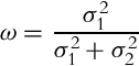
or after introducing ω2 = ω and ω1 = 1 − ω,
We are seeking the value of the weight ω that minimizes the variance that can be obtained from variance derivative:

which yields the solution
The minimum-variance estimate is therefore
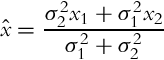
and the minimum variance is
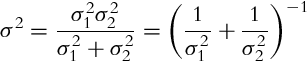
The obtained results confirm that the source with lower variance (higher belief) contributes more to the final estimate, and vice-versa.
Example 6.16
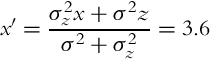
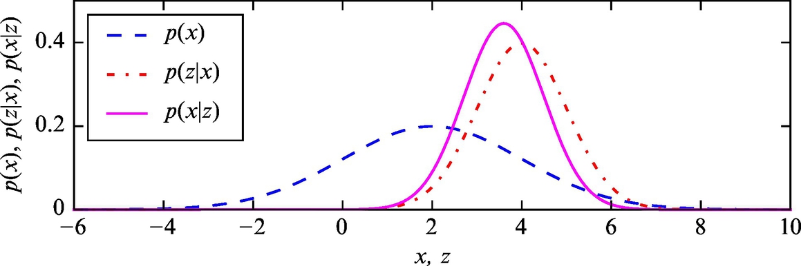
In a particular moment in time, an initial state estimate is given x = 2 with variance σ2 = 4. Then a sensor is used to measure the value of the state, which is z = 4 with sensor variance ![]() . The Gaussian probability distributions of the state and measurement are shown in Fig. 6.17.
. The Gaussian probability distributions of the state and measurement are shown in Fig. 6.17.

What is the value of optimum state estimate that includes information from previous state estimate and current measurement? What is the probability distribution of the updated optimum state estimate?
Solution
Based on Fig. 6.17 we can foreknow that the mean value x′ of the updated state will be closer to the measurement mean value, since the measurement variance (uncertainty) is lower than previous estimate variance. Using Eq. (6.31) the updated state estimate is obtained:
Variance of the updated estimate σ′2 is lower than both previous variances, since the integration of the previous estimate and measurement information lower the uncertainty of the updated estimate. The variance of the updated estimate is obtained from Eq. (6.32):

and the standard deviation is
The updated probability distribution p(x|z) of the state after the measurement-based correction is shown in Fig. 6.18.
Let us use the findings from Example 6.15 in the derivation of the recursive state estimation algorithm. In every time step a new state measurement z(k) = x(k) + n(k) is obtained by the sensor, where n(k) is the measurement noise. The measurement variance ![]() is assumed to be known. The updated optimum state estimate is a combination of the previous estimate
is assumed to be known. The updated optimum state estimate is a combination of the previous estimate ![]() and the current measurement z(k), as follows:
and the current measurement z(k), as follows:
The updated state variance is
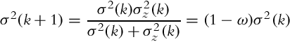
where
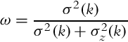
Therefore, given known initial state estimate x, ![]() and the corresponding variance σ2(0) the measurements z(1), z(2), … can be integrated optimally, in a way that the current state and state variance are estimated. This is the basic idea behind the correction step of the Kalman filter.
and the corresponding variance σ2(0) the measurements z(1), z(2), … can be integrated optimally, in a way that the current state and state variance are estimated. This is the basic idea behind the correction step of the Kalman filter.
The prediction step of the Kalman filter provides the given state prediction a known input action. The initial state estimate ![]() has a probability distribution with variance σ2(k). In the same way, the action u(k), which is responsible for transition of the state x(k) to x(k + 1), has probability distribution (transition uncertainty)
has a probability distribution with variance σ2(k). In the same way, the action u(k), which is responsible for transition of the state x(k) to x(k + 1), has probability distribution (transition uncertainty) ![]() . Using Example 6.17 let us examine the value of the state and the variance after the action is executed (after state transition).
. Using Example 6.17 let us examine the value of the state and the variance after the action is executed (after state transition).
Example 6.17
The initial state estimate ![]() with variance σ2(k) is known. Then an action u(k) is executed, which represents the direct transition of the state with uncertainty (variance)
with variance σ2(k) is known. Then an action u(k) is executed, which represents the direct transition of the state with uncertainty (variance) ![]() . What is the value of the state estimate and the state uncertainty after the transition?
. What is the value of the state estimate and the state uncertainty after the transition?
Solution
The updated state estimate after the transition is
and the uncertainty of this estimation is
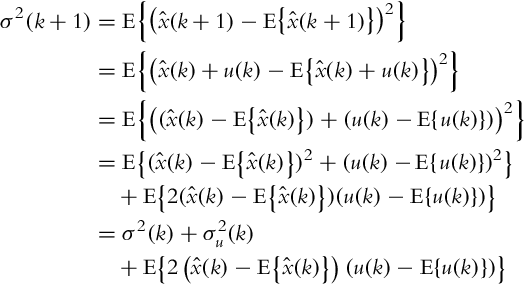
Since ![]() and u are independent, it holds
and u are independent, it holds ![]()
![]() , and therefore Eq. (6.33) simplifies to
, and therefore Eq. (6.33) simplifies to
Simplified Implementation of the Kalman Filter Algorithm
The Kalman filter algorithm for a simple case with only a single state is given in Algorithm 4, where the variables with a subscript (⋅)k|k−1 represent the estimated values in the prediction step, and variables with subscript (⋅)k|k represent the values from the correction step. For improved readability the following notation is used: u(k − 1) = uk−1 and z(k) = zk.
Algorithm 4
Kalman Filter for a Single State
functionKalman_filter(![]() , uk−1, zk,
, uk−1, zk, ![]() ,
, ![]() ,
, ![]() )
)
Prediction step:
![]()
![]()
Correction step:

![]()
![]()
return![]() ,
, ![]()
end function
The Kalman filter has two steps (prediction and correction step) that are executed one after another in the loop. In the prediction step only the known action is used in a way that enables prediction of the state in the next time step. From the initial belief a new belief is evaluated, and the uncertainty of the new belief is higher that the initial uncertainty. In the correction step the measurement is used to improve the predicted belief in a way that the new (corrected) state estimate has lower uncertainty than the previous belief. In both steps only two inputs are required: in the prediction step the value of previous belief ![]() and executed action uk−1 need to be known, and in the correction step the previous belief
and executed action uk−1 need to be known, and in the correction step the previous belief ![]() and measurement zk are required. The state transition variance
and measurement zk are required. The state transition variance ![]() , input action variance
, input action variance ![]() , and measurement variance
, and measurement variance ![]() also need to be given.
also need to be given.
Example 6.18
There is a mobile robot that can move in only one dimension. The initial position of the robot is unknown (Fig. 6.19). Let us therefore assume that the initial position is ![]() with large variance
with large variance ![]() (the true position x0 = 0 is not known).
(the true position x0 = 0 is not known).

Then, in every time moment k − 1 = 0, …, 4 the mobile robot is moved for u0:4 = (2, 3, 2, 1, 1) units and the measurements of the robot positions in time moments k = 1, …, 5 are taken, z1:5 = (2, 5, 7, 8, 9). The movement action and measurement are disturbed with white normally distributed zero-mean noise that can be described with a constant uncertainty for movement ![]() and measurement uncertainty
and measurement uncertainty ![]() .
.
What is the estimated robot position and uncertainty of this estimate?
Solution
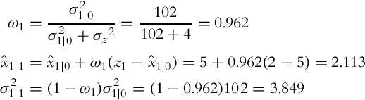
Let us apply Algorithm 4 to solve the given mobile robot localization problem. In the initial time step (k = 1) the predicted state and variance can be calculated first:

and then the correction step of the Kalman filter in the first time step k = 1 can be evaluated:
These prediction and correction steps can be evaluated for all the other time steps. The prediction results are therefore

and the correction results are
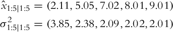
The obtained results show that the position of the mobile robot can be determined in a few time steps with uncertainty 2, which agrees with the prediction uncertainty and measurement uncertainty  . The uncertainty of the predicted position estimate converges toward 4, which is in accordance with the correction uncertainty from the previous time step and measurement
 ![]() .
.
6.5.1 Kalman Filter in Matrix Form
Multiple input, multiple state, and multiple output systems can be represented in a matrix form for improved readability. A general linear system can be expressed in a state-space form as
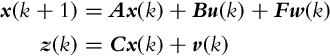
where x is the state vector, u is the input (action) vector, and z is the output (measurement); A is the state matrix, B is the input matrix, F is the input noise matrix, C is the output matrix; w(k) is the process noise and v is the output (measurement) noise. In the case the noise w is added to the system input u, the following relation holds: F = B. The process noise w(k) and measurement noise v(k) are assumed to be independent (uncorrelated) white noises with zero mean value and covariance matrices ![]() and
and ![]() .
.
The probability distribution of the states x that are disturbed by a white Gaussian noise can be written in a matrix form as follows:
where P is the state-error covariance matrix.
The Kalman filter is an approach for filtering and estimation of linear systems with continuous state space, which are disturbed with normal noise. The noise distribution is represented with a Gaussian function (Gaussian noise). The input and measurement noises influence the internal system states that we would like to estimate. In the case that the model of the system is linear, the Gaussian noise propagated through the model (e.g., from inputs to the states) is also a Gaussian noise. The system must therefore be linear, since this requirement ensures Gaussian distribution of the noise on the states, an assumption used in the derivation of the Kalman filter. The Kalman filter state estimate converges to the true value only in the case of linear systems that are disturbed with Gaussian noise.
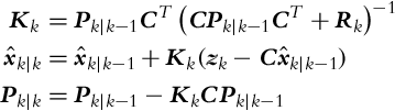
The Kalman filter for a linear system (6.34) has a prediction step:
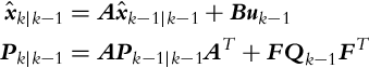
and a correction step:
In the prediction part of the algorithm the a priori estimate ![]() is determined, which is based on the previous estimate
is determined, which is based on the previous estimate ![]() (obtained from measurements up to the time moment k − 1) and input u(k − 1). In the correction part of the Kalman filter the posteriori estimate
(obtained from measurements up to the time moment k − 1) and input u(k − 1). In the correction part of the Kalman filter the posteriori estimate ![]() is calculated, which is based on the measurements up to time step k. The state correction is made in a way that the difference between the true and estimated measurement is calculated (
is calculated, which is based on the measurements up to time step k. The state correction is made in a way that the difference between the true and estimated measurement is calculated (![]() ); this difference is also known as innovation or measurement residual. The state correction is calculated as a product of Kalman gain Kk and innovation. The prediction part can be evaluated in advance, in the time while we are waiting for the new measurement in the time step k. Notice the similarity of the matrix notation in Eqs. (6.35), (6.36) with the notation used in Algorithm 4.
); this difference is also known as innovation or measurement residual. The state correction is calculated as a product of Kalman gain Kk and innovation. The prediction part can be evaluated in advance, in the time while we are waiting for the new measurement in the time step k. Notice the similarity of the matrix notation in Eqs. (6.35), (6.36) with the notation used in Algorithm 4.
Let us derive the equation for the calculation of the state error covariance matrix in the prediction part of the Kalman filter:
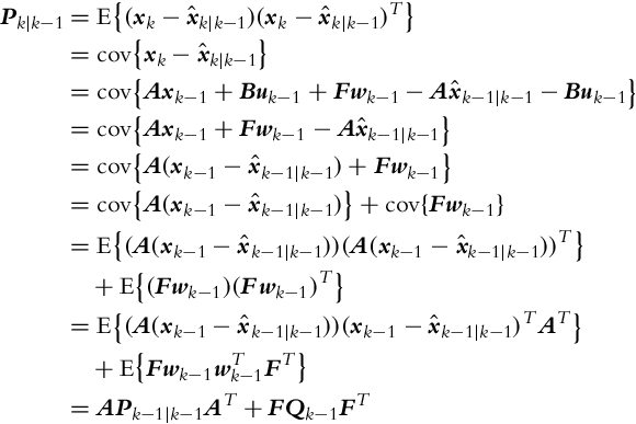
where in line six of the derivation we took into account that the process noise wk in time step k is independent of the state estimate error in the previous time step (![]() ).
).
Let us also derive the equation for computation of the state error covariance matrix in the correction part of the Kalman filter:
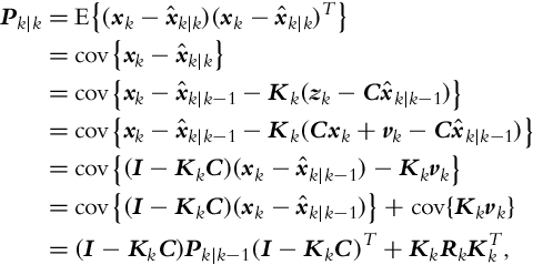
where in line six of the derivation we took into account that the measurement noise vk is uncorrelated with the other terms. The obtained relation for calculation of the covariance matrix Pk|k is general and can be used for arbitrary gain Kk. However, the expression for Pk|k in Eq. (6.36) is valid only for optimum gain (Kalman gain) that minimizes the mean squared correction error ![]() ; this is equivalent to the minimization of the sum of all the diagonal elements in the correction covariance matrix Pk|k.
; this is equivalent to the minimization of the sum of all the diagonal elements in the correction covariance matrix Pk|k.
The general equation for Pk|k can be extended and the terms rearranged:
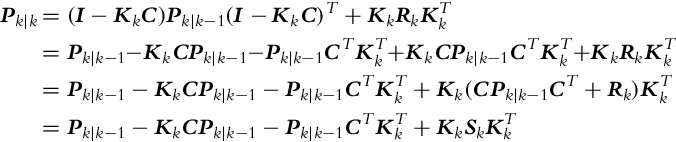
where Sk = CPk|k−1CT +Rk represents the innovation covariance matrix (![]() ). The sum of the diagonal terms of Pk|k is minimal when the derivative of Pk|k with respect to Kk is zero:
). The sum of the diagonal terms of Pk|k is minimal when the derivative of Pk|k with respect to Kk is zero:
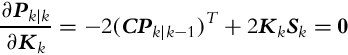
which leads to the optimum gain in Eq. (6.36):
The correction covariance matrix at optimum gain can be derived if the optimum gain is postmultiplied with ![]() and inserted into the equation for Pk|k:
and inserted into the equation for Pk|k: