3.3.8 Model-Based Predictive Control

Model-based predictive control (MPC) approaches are advanced methods that can be applied to various areas as well as to mobile robotics were reference trajectory is known beforehand. The use of predictive control approaches in mobile robotics usually relies on a linearized (or also nonlinear) kinematic model or dynamic model to predict future system states. A number of successful implementations to wheeled robotics have been reported such as generalized predictive control in [18], predictive control with Smith predictor to handle the system’s time delay in [19], MPC based on a linear, time-varying system description in [20], nonlinear predictive controller with a multilayer neural network as a system model in [21], and many others. In most approaches the control law solutions are solved by an optimization of a cost function. Other approaches obtain control law as an analytical solution, which is computationally effective and can be easily used in fast, real-time implementations [22].

This section deals with a differentially driven mobile robot and trajectory-tracking control. Reference trajectory needs to be a smooth twice-differentiable function of time. For prediction, a linearized error dynamics model obtained around the reference trajectory is used. The controller minimizes the difference between the robot future tracking error and the reference error with defined desired dynamics.

Model-based control strategies combine a feedforward solution and a feedback action in input vector u, given as follows:

$\begin{array}{l}\hfill \mathit{u}={\mathit{u}}_{\mathrm{ff}}+{\mathit{u}}_{\mathrm{fb}}=\left[\begin{array}{l}{v}_{\mathrm{ref}}cos{e}_{\phi }+v_{\mathrm{fb}}\\ {\omega }_{\mathrm{ref}}+{\omega }_{\mathrm{fb}}\\ \end{array}\right]\end{array}$

where the feedforward input vector ${\mathit{u}}_{\mathrm{ff}}={[v_{\mathrm{ref}}cos{e}_{\phi }{\omega }_{\mathrm{ref}}]}^T$ is calculated from the reference trajectory using relations (3.22), (3.23). The feedback input vector is u_fb = [v_fbω_fb]^T, which is the output of the MPC controller.

The control problem is given by the linear tracking error dynamics model (3.39), which in shorter notation reads

$\begin{array}{l}\hfill \dot{\mathit{e}}={\mathit{A}}_{\mathrm{c}}(t)\mathit{e}+{\mathit{B}}_{\mathrm{c}}{\mathit{u}}_{\mathrm{fb}}\end{array}$

where A_c(t) and B_c are matrices of the continuous state-space model and e is the tracking error defined in local robot coordinates, defined by transformation (3.35) and shown in Fig. 3.21.

Discrete MPC

The MPC approach presented in [22] is summarized. It is designed for discrete time; therefore, model (3.86) needs to be written in discrete-time form:

$\begin{array}{l}\hfill \dot{\mathit{e}}(k+1)=\mathit{A}(k)\mathit{e}(k)+\mathit{B}{\mathit{u}}_{\mathrm{fb}}(k)\end{array}$

  (3.87)

where $\mathit{A}(k)\in {\mathbb{R}}^n\times {\mathbb{R}}^n$, n is the number of the state variables and $\mathit{B}\in {\mathbb{R}}^n\times {\mathbb{R}}^m$, and m is the number of input variables. The discrete matrices A(k) and B can be obtained as follows:

$\begin{array}{l}\hfill \begin{array}{cc}\mathit{A}(k)& =\mathit{I}+{\mathit{A}}_{\mathrm{c}}(t)T_{\mathrm{s}}\\ \mathit{B}& ={\mathit{B}}_{\mathrm{c}}{T}_{\mathrm{s}}\end{array}\end{array}$

  (3.88)

which is sufficient approximation for a short sampling time T_s.

The main idea of MPC is to compute optimal control actions that minimize the objective function given in prediction horizon interval h. The objective function is a quadratic cost function:

$\begin{array}{l}\hfill J({\mathit{u}}_{\mathrm{fb}},k)=\sum _{i=1}^h{\mathit{ϵ}}^T(k,i)\mathit{Q}\mathit{ϵ}(k,i)+{\mathit{u}}_{\mathrm{fb}}^T(k+i-1)\mathit{R}{\mathit{u}}_{\mathrm{fb}}(k+i-1)\end{array}$

  (3.89)

consisting of a future reference tracking error e_r(k + i), predicted tracking error e(k + i|k), difference between the two errors ϵ(k, i) =e_r(k + i) −e(k + i|k), and future actions u_fb(k + i − 1), where i denotes the ith step-ahead prediction (i = 1, …, h). Q and R are the weighting matrices.

For prediction of the state e(k + i|k) the error model (3.87) is applied as follows:

$\begin{array}{l}\hfill \begin{array}{cc}\mathit{e}(k+1|k)& =\mathit{A}(k)\mathit{e}(k)+\mathit{B}{\mathit{u}}_{\mathrm{fb}}(k)\\ \mathit{e}(k+2|k)& =\mathit{A}(k+1)\mathit{e}(k+1|k)+\mathit{B}{\mathit{u}}_{\mathrm{fb}}(k+1)\\ & ⋮\\ \mathit{e}(k+i|k)& =\mathit{A}(k+i-1)\mathit{e}(k+i-1|k)+\mathit{B}{\mathit{u}}_{\mathrm{fb}}(k+i-1)\\ & ⋮\\ \mathit{e}(k+h|k)& =\mathit{A}(k+h-1)\mathit{e}(k+h-1|k)+\mathit{B}{\mathit{u}}_{\mathrm{fb}}(k+h-1)\end{array}\end{array}$

  (3.90)

Predictions e(k + i|k) in Eq. (3.90) are rearranged so that they are dependent on current error e(k), current and future inputs u_fb(k + i − 1), and matrices A(k + i − 1) and B. The model-output prediction at the time instant h can then be written as

$\begin{array}{l}\hfill \begin{array}{cc}\mathit{e}(k+h|k)& ={\mathrm{\Pi }}_{j=1}^{h-1}\mathit{A}(k+j)\mathit{e}(k)+\\ & +\sum _{i=1}^h\left({\mathrm{\Pi }}_{j=i}^{h-1}\mathit{A}(k+j)\right)\mathit{B}{u}_{\mathrm{fb}}(k+i-1)+\mathit{B}{\mathit{u}}_{\mathrm{fb}}(k+h-1)\end{array}\end{array}$

  (3.91)

The future reference error (e_r(k + i)) defines how the tracking error should decrease when the robot is not on the trajectory. Let us define the future reference error to decrease exponentially from the current tracking error e(k), as follows:

$\begin{array}{l}\hfill {\mathit{e}}_r(k+i)={\mathit{A}}_r^{i}e(k)\end{array}$

  (3.92)

for $i=1,\dots ,h$. The dynamics of the reference error is defined by the reference model matrix A_r.

According to Eqs. (3.90), (3.91) the robot-tracking prediction-error vector is defined as follows:

$\begin{array}{l}\hfill {\mathit{E}}^{*}(k)={\left[\mathit{e}{(k+1|k)}^T\mathit{e}{(k+2|k)}^T\dots \mathit{e}{(k+h|k)}^T\right]}^T\end{array}$

where E* is given for the whole interval of the observation (h) where the control vector is

$\begin{array}{l}\hfill {\mathit{U}}_{\mathrm{fb}}(k)={\left[{\mathit{u}}_{\mathrm{fb}}^T(k){\mathit{u}}_{\mathrm{fb}}^T(k+1)\dots {\mathit{u}}_{\mathrm{fb}}^T(k+h-1)\right]}^T\end{array}$

  (3.93)

and

$\begin{array}{l}\hfill \mathbf{\Lambda }(k,i)={\mathrm{\Pi }}_{j=i}^{h-1}\mathit{A}(k+j)\end{array}$

The robot-tracking prediction-error vector can be written in compact form:

$\begin{array}{l}\hfill {\mathit{E}}^{*}(k)=\mathit{F}(k)\mathit{e}(k)+\mathit{G}(k){\mathit{U}}_{\mathrm{fb}}(k)\end{array}$

  (3.94)

where

$\begin{array}{l}\hfill \mathit{F}(k)={\left[\mathit{A}(k)\mathit{A}(k+1)A(k)\dots \mathbf{\Lambda }(k,0)\right]}^T\end{array}$

  (3.95)

and

$\begin{array}{l}\hfill \mathit{G}(k)=\left[\begin{array}{llll}\mathit{B}& 0& \cdots & 0\\ \mathit{A}(k+1)\mathit{B}& \mathit{B}& \cdots & ⋮\\ ⋮& ⋮& \ddots & ⋮\\ \mathbf{\Lambda }(k,1)\mathit{B}& \mathbf{\Lambda }(k,2)\mathit{B}& \cdots & \mathit{B}\end{array}\right]\end{array}$

  (3.96)

where dimensions of F(k) and G(k) are (n ⋅ h × n) and (n ⋅ h × m ⋅ h), respectively.

The robot reference-tracking-error vector is

$\begin{array}{l}\hfill {\mathit{E}}_r^{*}(k)={\left[{\mathit{e}}_r{(k+1)}^T{\mathit{e}}_r{(k+2)}^T\dots {\mathit{e}}_r{(k+h)}^T\right]}^T\end{array}$

which in compact form is computed as

$\begin{array}{l}\hfill {\mathit{E}}_r^{*}(k)={\mathit{F}}_{r}e(k)\end{array}$

  (3.97)

where

$\begin{array}{l}\hfill {\mathit{F}}_r={\left[{\mathit{A}}_r{\mathit{A}}_r{A}_r^2\dots {\mathit{A}}_r{A}_r^h\right]}^T\end{array}$

  (3.98)

where F_r is the (n ⋅ h × n) matrix.

The optimal control vector (3.93) is obtained by optimization of Eq. (3.89), which can be done numerically or analytically. The analytical solution is derived in the following.

The objective function (3.89) defined in matrix form reads.

$\begin{array}{l}\hfill J({\mathit{U}}_{\mathrm{fb}})={\left({\mathit{E}}_r^{*}-{\mathit{E}}^{*}\right)}^T\overline{\mathit{Q}}\left({\mathit{E}}_r^{*}-{\mathit{E}}^{*}\right)+{\mathit{U}}_{\mathrm{fb}}^T\overline{\mathit{R}}{\mathit{U}}_{\mathrm{fb}}\end{array}$

  (3.99)

The minimum of Eq. (3.99) is expressed as

$\begin{array}{l}\hfill \frac{\partial J}{\partial {\mathit{U}}_{\mathrm{fb}}}=-2\overline{\mathit{Q}}{\mathit{G}}^T{\mathit{E}}_r^{*}+2{\mathit{G}}^T\overline{\mathit{Q}}{\mathit{E}}^{*}+2\overline{\mathit{R}}{\mathit{U}}_{\mathrm{fb}}=0\end{array}$

  (3.100)

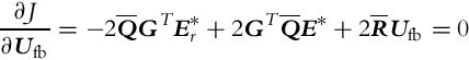
and the solution for the optimal control vector is obtained as

$\begin{array}{l}\hfill {\mathit{U}}_{\mathrm{fb}}(k)={\left({\mathit{G}}^T\overline{\mathit{Q}}\mathit{G}+\overline{\mathit{R}}\right)}^{-1}{\mathit{G}}^T\overline{\mathit{Q}}\left({\mathit{F}}_r-\mathit{F}\right)\mathit{e}(k)\end{array}$

  (3.101)

where the weighting matrices are as follows:

$\begin{array}{l}\hfill \overline{\mathit{Q}}=\left[\begin{array}{llll}\mathit{Q}& 0& \cdots & 0\\ 0& \mathit{Q}& \cdots & 0\\ ⋮& ⋮& \ddots & ⋮\\ 0& 0& \cdots & \mathit{Q}\end{array}\right]\end{array}$

  (3.102)

and

$\begin{array}{l}\hfill \overline{\mathit{R}}=\left[\begin{array}{llll}\mathit{R}& 0& \cdots & 0\\ 0& \mathit{R}& \cdots & 0\\ ⋮& ⋮& \ddots & ⋮\\ 0& 0& \cdots & \mathit{R}\end{array}\right]\end{array}$

  (3.103)

Solution (3.101) contains control vectors u_fb^T(k + i − 1) for the whole interval of prediction (i = 1, …, h). To apply feedback control action in the current time instant k only the first vector u_fb^T(k) (first m rows of U_fb(k)) is applied to the robot. The solution is obtained analytically; therefore, it enables fast real-time implementations that may not be possible if numeric optimization of Eq. (3.89) is used.

Example 3.13

Implement model predictive control given in Eq. (3.101) for trajectory tracking of a differential-drive robot. Reference trajectory and robot are defined in Example 3.9.

The choice for prediction horizon is h = 4, the reference model matrix is A_r = I_3×3 ⋅ 0.65, and the weighting matrices are

$\begin{array}{l}\hfill \mathit{Q}=\left[\begin{array}{lll}4& 0& 0\\ 0& 40& 0\\ 0& 0& 0.1\end{array}\right],\mathit{R}=I_{2\times 2}\cdot 10^{-3}\end{array}$

Solution

Using MPC compute the feedback part of control signal u_fb(k) and apply it to the robot together with the feedforward part u_ff(k). In the following Matlab script (Listing 3.12), possible solution and trajectory tracking results are given. Obtained simulation results are shown in Figs. 3.30 and 3.31.

Listing 3.12

1 Ts =  0.033;   %  Sampling time

2 t  =   0: Ts : 3 0 ;   %  Simulation time

3 q  =   [ 1 . 1 ;   0 . 8 ;   0 ] ;   %   Initial  robot pose

4

5 %  Reference

6 freq   =  2*pi/30;

7   xRef  =   1.1   +  0.7*sin( freq *t ) ;  yRef  =   0.9   +  0.7*sin(2* freq *t ) ;

8  dxRef  =   freq *0.7*cos( freq *t ) ;  dyRef  =  2* freq *0.7*cos(2* freq *t ) ;

9 ddxRef =− freq ˆ2*0.7* sin( freq *t ) ;  ddyRef  =−4* freq ˆ2*0.7* sin (2* freq *t ) ;

10 qRef  =   [ xRef ;  yRef ;  atan2( dyRef ,  dxRef ) ] ;   %  Reference trajectory

11 vRef  =  sqrt( dxRef.ˆ2+dyRef .ˆ2) ;

12 wRef  =  ( dxRef .* ddyRef− dyRef .* ddxRef ) . / ( dxRef .ˆ2+dyRef .ˆ2) ;

13 uRef  =   [ vRef ;  wRef ] ;   %  Reference inputs

14

15 for k  =   1:length( t )−4

16     e   =   [ cos ( q (3) ) , sin(q (3) ) ,  0;   . . .

17       − sin ( q (3) ) ,  cos(q (3) ) ,  0;   . . .

18        0 , 0 ,  1]*( qRef ( : , k)  −   q ) ;   %  Error vector

19     e (3)   =  wrapToPi( e (3) ) ;   %  Correct angle

20

21     A0  =   [1 ,  Ts*uRef (2 ,k) ,  0;− Ts * uRef (2 , k) , 1 , Ts*uRef (1 ,k) ;   0 ,0 ,1];

22     A1  =   [1 ,  Ts*uRef (2 ,k+1) ,  0;− Ts * uRef (2 , k+1) , 1 , Ts*uRef (1 ,k+1) ;   0 ,0 ,1];

23     A2  =   [1 ,  Ts*uRef (2 ,k+2) ,  0;− Ts * uRef (2 , k+2) , 1 , Ts*uRef (1 ,k+2) ;   0 ,0 ,1];

24     A3  =   [1 ,  Ts*uRef (2 ,k+3) ,  0;− Ts * uRef (2 , k+3) , 1 , Ts*uRef (1 ,k+3) ;   0 ,0 ,1];

25     A4  =   [1 ,  Ts*uRef (2 ,k+4) ,  0;− Ts * uRef (2 , k+4) , 1 , Ts*uRef (1 ,k+4) ;   0 ,0 ,1];

26     B   =   [ Ts ,   0;  0 ,  0;  0 , Ts ] ;

27     C   =  eye(3) ;

28

29     Z  =  zeros(3 ,2) ;

30     Hm   =   [C *A0*B,  Z,  Z,  Z;   . . .

31     C *A0*A1*B,   C *A0*B,  Z,  Z;   . . .

32     C *A0*A1*A2*B,   C *A0*A1*B,   C *A0*B,  Z;   . . .

33     C *A0*A1*A2*A3*B,   C *A0*A1*A2*B,   C *A0*A1*B,   C *A0* B] ;

34     Fm   =   [C *A0*A1,   C *A0*A1*A2,   C *A0*A1*A2*A3,   C *A0*A1*A2*A3*A4 ] . ’ ;

35

36     ar  =   0.65;

37     Ar  =  eye(3) *ar ;   %  Reference error dynamics

38     H   =   0;

39     Fr  =   [ Arˆ(H +1) , Arˆ(H +2) , Arˆ(H +3) , Arˆ(H +4) ] . ’ ;

40

41     %  Weight matrices

42     Qt  =  diag( repmat ( [ 1 ;   40;   0 . 1 ] ,  4 , 1) ) ;

43     Rt  =  diag( repmat ( [ 0 . 0 0 1 ;   0.001] ,  4 , 1) ) ;

44

45     %  Optimal control calculation

46     KKgpc  =  ( Hm. ’*Qt* Hm   +  Rt) ∖( Hm. ’*Qt *(− Fm ) ) ;

47     KK   =  KKgpc ( 1 : 2 , : ) ;   %  Take current control gains

48

49     v  =  − KK * e ;

50     uF   =   [ uRef (1 ,k)*cos( e (3) ) ;  uRef (2 ,k) ] ;

51     u  =  v  +  uF;

52

53     vMAX   =   1;   wMAX   =   15;   %  Max   velocities

54     if  abs(u(1) ) > vMAX ,  u(1)   =  sign(u(1) )* vMAX;  end

55     if  abs(u(2) ) > wMAX ,  u(2)   =  sign(u(2) )* wMAX;  end

56

57     %  Robot motion simulation

58     dq  =   [ u(1) *cos(q (3) ) ;  u(1) *sin(q (3) ) ;  u(2) ] ;

59     noise   =   0.00;   %  Set to experiment with noise (e.g. 0.001)

60     q  =  q  +  Ts*dq  +  randn(3 ,1) * noise ;   %  Euler integration

61     q (3)   =  wrapToPi(q (3) ) ;   %  Map  orientation angle to [− pi , pi]

62 end

3.3.9 Particle Swarm Optimization-Based Control

Control of a mobile robot can also be defined as an optimization problem where the best solution among all possible solutions in a search space needs to be found in each control-loop sample time. The obtained control does not have an explicit structure, meaning that the control law cannot be given as a mapping function from system states to control actions. An optimal solution that minimizes some objective function is instead found by an iterative optimization algorithm like Newton methods, gradient descent methods, or stochastic methods such as genetic algorithms, particle swarm optimization (PSO), and the like.

If the objective function is not convex in the minimization problem then most optimization algorithms can be trapped in a local minimum, which is not the optimal solution. Using stochastic optimization the likelihood of local minimum, the solution is usually smaller because the search pattern is randomized to some extent.

PSO is inspired by social behavior of small animals such as bird flocks or fish schools [23, 24]. PSO uses a group (swarm) of particles where each particle presents its own solution hypothesis. Each particle i is characterized by parameter vector x_i defining its position in the parameter space and increment vector v_i defining velocity in the parameter space. During optimization the population of all candidate solutions are updated according to the objective function that defines a measure of quality. Each particle keeps track of its parameters and remembers the best parameters pBest_i achieved so far together with the associated objective function J_i = f(pBest_i). During optimization also the best parameter vector obtained so far for the entire swarm gBest is stored. In local version of PSO for each particle the best parameter vector gBest_i is tracked for some neighborhood of particles (e.g., k nearest particles, ring topology, and the like [25]). Local versions of PSO are less likely to be trapped in a local minimum.

Next, a basic (global) version of PSO is explained. In each control-loop iteration particles update mimic cognitive and social behavior by means of the following rules:

$\begin{array}{l}\hfill \begin{array}{cc}& {\mathit{v}}_i\leftarrow \omega {\mathit{v}}_i+c_1{\text{rand}}_{(0,1)}({\text{pBest}}_i-{\mathit{x}}_i)+c_2{\text{rand}}_{(0,1)}(\text{gBest}-{\mathit{x}}_i)\\ & {\mathit{x}}_i\leftarrow {\mathit{x}}_i+{\mathit{v}}_i\end{array}\end{array}$

where ω is the inertia factor, c₁ is the self-cognitive constant, and c₂ is the social constant. In addition rand_{(0, 1)} is a vector of uniformly distributed values in the range (0, 1). The dimensions of vectors in Eq. (3.104) equal the dimension of the parameter search space. The parameters ω, c₁, and c₂ are positive tuning parameters. Basic PSO code is given in Algorithm 1.

Example 3.14

Write the controller using the PSO for the robot and trajectory defined in Example 3.9. PSO is applied in each sampling time t = kT_s to find the best controls (translational and angular velocity) that would drive the robot as close as possible to the current reference position x_ref(t), y_ref(t). Next, the robot pose prediction is computed considering robot kinematics and the particles’ proposed solution (control action). Optimal control minimizes the cost function consisting of the tracking error $\mathit{e}(t)={\left[e_x(t),e_y(t),e_{\phi }(t)\right]}^T$ and the feedback control effort ${\mathit{u}}_{\mathrm{fb}}={\left[v_{\mathrm{fb}},{\omega }_{\mathrm{fb}}\right]}^T$. This follows the equation J(t) = e(t)^TQe(t) +u_fb^TRu_fb, where Q and R are diagonal weighting matrices used to tune the controller behavior.

Solution

The control law includes feedforward action and feedback action similarly as in Example 3.9. Feedforward action is obtained from a known trajectory while the feedback action is computed using PSO. The tracking error is expressed in robot local coordinates (see Fig. 3.21) because this makes the optimization more efficient due to the closed-loop system being decoupled better. The error in the local x coordinate can simply be compensated by translational velocity, and errors in y and φ can be compensated by the angular velocity. However, this is not the case when using a global tracking error due to nonlinear rotation transformation in Eq. (3.35).

In Listing 3.13 a Matlab script of a possible solution is given. Obtained simulation results are shown in Figs. 3.32 and 3.33. Similar control results as in Example 3.13 are obtained. However, the computational effort is much higher than in Example 3.13. Results of Example 3.14 are not deterministic because PSO is using randomly distributed particles in optimization to find the best control in each sampling time. Therefore, resulting trajectories of the mobile robot can vary to some extent, especially the initial transition phase, until the robot reaches the reference. However, the obtained results in the majority of simulation runs are at least comparable to the results of other presented deterministic controllers (e.g., from Example 3.9).

Listing 3.13

1 Ts =  0.033;   %  Sampling time

2 t  =   0: Ts : 3 0 ;   %  Simulation time

3 q  =   [ 1 . 1 ;   0 . 8 ;   0 ] ;   %   Initial  robot pose

4

5 %  Reference

6 freq   =  2*pi/30;

7   xRef  =   1.1   +  0.7*sin( freq *t ) ;  yRef  =   0.9   +  0.7*sin(2* freq *t ) ;

8  dxRef  =   freq *0.7*cos( freq *t ) ;  dyRef  =  2* freq *0.7*cos(2* freq *t ) ;

9 ddxRef =− freq ˆ2*0.7* sin( freq *t ) ;  ddyRef  =−4* freq ˆ2*0.7* sin (2* freq *t ) ;

10 qRef  =   [ xRef ;  yRef ;  atan2( dyRef ,  dxRef ) ] ;   %  Reference trajectory

11 vRef  =  sqrt( dxRef.ˆ2+dyRef .ˆ2) ;

12 wRef  =  ( dxRef .* ddyRef− dyRef .* ddxRef ) . / ( dxRef .ˆ2+dyRef .ˆ2) ;

13 uRef  =   [ vRef ;  wRef ] ;   %  Reference inputs

14

15 vMax  =   1;   wMax   =   15;   %  Velocity constraints

16

17 %  Swarm   Initial i z a t i o n

18 i t e r a t i o n s   =   20;   %  Number of  i t e r a t i o n s

19 omega  =   0.5*0.5;   %  Inertia

20 c1  =   0.5*1;   %  Correction factor

21 c2  =   0.5*1;   %  Global correction factor

22 N   =   25;   %  Swarm   s i z e

23 swarm  =  zeros([2 ,N, 4 ] ) ;

24 uBest  =   [ 0 ;   0 ] ;

25

26 for k  =   1:length( t )−1

27     %   Initial  swarm position

28     swarm ( : , : , 1 )   =  repmat ( uBest ,  1 ,  N)  +  diag ( [ 0 . 1 ;   3]) *randn(2 ,N) ;

29     swarm ( : , : , 2 )   =   0;   %   Initial   p a r t i c l e  velocity

30     swarm (1 ,: ,4)   =  1000;  %  Best value so far

31

32     for  i t e r   =   1: i t e r a t i o n s   %  PSO   i t e r a t i v e l y  find best solution

33        %  Evaluate  p a r t i c l e s  parameters

34        for  i   =   1:N

35          %  Compute new predicted pose of the robot using i − th   p a r t i c l e

36          %  parameters (input  velocities ) and compare obtained predicted

37          %  pose to the reference pose.

38          vwi  =  swarm ( : , i ,1) ;

39          ui  =  vwi  +  uRef ( : , k) ;   %  Feedback and feedforward

40          qk  =  q ;   %  Current robot pose

41          %  Predict robot pose using  p a r t i c l e  parameters ( velocities )

42          qk  =  qk  +  Ts *[cos(qk (3) ) ,  0;  sin(qk (3) ) ,  0;  0 ,  1]* ui ;

43          qk (3)   =  wrapToPi(qk (3) ) ;   %  Correct angle range

44          e  =   [cos(qk (3) ) , sin(qk (3) ) ,  0;   . . .

45             − sin ( qk (3) ) , cos(qk (3) ) ,  0;   . . .

46             0 , 0 ,  1]*( qRef ( : , k+1) − qk ) ;   %  Error

47          e (3)   =  wrapToPi( e (3) ) ;   %  Correct angle range

48          Qt  =  diag ( [ 4 ;   80;   0 . 1 ] ) ;  Rt  =  diag ( [ 1 ;   1]*0.0001) ;   %  Weights

49          J  =  e . ’*Qt*e  +  vwi . ’* Rt*vwi ;   %  Cost function

50          if  J < swarm(1 , i ,4)   %  if  new parameter  i s  better , update:

51            swarm ( : , i ,3)   =  swarm ( : , i ,1) ;   %  param values (v and w )

52            swarm(1 , i ,4)   =  J ;   %  and best  c r i t e r i a  value.

53       end

54     end

55     [˜ ,  gBest ]   =  min(swarm (1 ,: ,4) ) ;   %  Global best  p a r t i c l e  parameters

56

57     %  Updating parameters by velocity vectors

58     a  =  omega*swarm ( : , : , 2 )   +   . . .

59     c1*rand(2 ,N) .*( swarm ( : , : , 3 )  −   swarm ( : , : , 1 ) )   +   . . .

60     c2*rand(2 ,N) .*( repmat (swarm ( : , gBest ,3) , 1 ,  N)  −   swarm ( : , : , 1 ) ) ;

61     %  Max  param increment , acceleration: aMax =3  ==>  3*Ts=0.1

62     a (1 , a ( 1 , : ) >0.1)  =   0 . 1 ;  a (1 , a ( 1 , : ) <−0.1)   =   −0.1;

63     %  Max  param increment , angular acceleration: aMax =60 ==>  60*Ts=2

64     a (2 , a ( 1 , : ) >2)  =   2;  a (2 , a ( 1 , : ) <−2)   =   −2;

65

66     v   =   swarm ( : , : , 1 )   +   a ;  %  Update velocity

67     %  Limit velocity to preserve curvature  . . .

68     [m,   i i ]   =  max ( [ v ( 1 , : ) /vMax;  v ( 2 , : ) / wMax;  ones (1 ,N) ] ) ;

69     i   =   i i ==1; v(1 , i )  =  sign(v(1 , i ) )*vMax;

70        v(2 , i )  =  v(2 , i ) ./m ( i ) ;

71     i   =   i i ==2; v(2 , i )  =  sign(v(2 , i ) )* wMax;

72        v(1 , i )  =  v(1 , i ) ./m ( i ) ;

73    

74     swarm ( : , : , 2 )   =  a ;   %  Updated  p a r t i c l e   velocities  (acceleration)

75     swarm ( : , : , 1 )   =  v ;   %  Updated  p a r t i c l e  positions ( velocities )

76   end

77

78   %  Take the best  p a r t i c l e  to get robot command   velocities

79   uBest  =  swarm ( : , gBest ,1) ;

80   u  =  uBest  +  uRef ( : , k) ;   %  Feedback and feedforward

81

82   %  Velocity constraints

83   if  abs(u(1) ) > vMax,  u(1)   =  sign(u(1) )*vMax;  end

84   if  abs(u(2) ) > wMax,  u(2)   =  sign(u(2) )* wMax;  end

85  

86   %  Robot motion simulation

87   dq  =   [ u(1) *cos(q (3) ) ;  u(1) *sin(q (3) ) ;  u(2) ] ;

88   noise   =   0.00;   %  Set to experiment with noise (e.g. 0.001)

89   q  =  q  +  Ts*dq  +  randn(3 ,1) * noise ;   %  Euler integration

90   q (3)   =  wrapToPi(q (3) ) ;   %  Map  orientation angle to [− pi , pi]

91 end

PSO is a generic algorithm that can be applied to numerous applications as long as the computational effort and time required to find the solution meet the real time requirements of the system being controlled.

MPC With PSO

Solving optimization of objective function in MPC can also be done by PSO, where the best parameters (control actions) are searched for the prediction interval (t, t + hT_S) where h is horizon. If a system has m = 2 control inputs then the optimization needs to find m ⋅ h optimal parameters, which may be computationally intense and therefore problematic for systems with short control-loop sampling times. However, there are some possibilities to lower the computational time as follows. One possibility is to assume constant controls in the prediction horizon. If the control action does not change significantly in a relatively short horizon time, then constant controls can be assumed in the horizon interval. This means that only m parameters instead of m ⋅ h need to be optimized. Another possibility is to lower the required iterations in optimization for each control-loop sampling time. This can be done by initializing the particles around the optimal solution from the previous time sample. Doing so, this would hopefully require less iterations for the particles to converge.

A possible solution of implementing MPC on PSO is given in Example 3.15.

Example 3.15

Extend Example 3.14 to a model-based predictive controller with prediction horizon h = 3.

Solution

The presented solution supposes that the control action (feedback part) in the prediction horizon interval is constant u_fb(t + (i − 1)T_S) =u_fb. Feedforward action (u_ff) is obtained from known trajectory, while the feedback action is computed using PSO. From the current robot pose the h-step-ahead prediction is made using the robot kinematic model and control actions u(t + (i − 1)T_S) =u_fb +u_ff(t + (i − 1)T_S) (i = 1, …, h) are obtained as follows:

$\begin{array}{l}\hfill \widehat{\mathit{q}}(t+i{T}_S)=f\left(\widehat{\mathit{q}}\left(t+\left(i-1\right)T_S\right),\mathit{u}\left(t+\left(i-1\right)T_S\right)\right)\end{array}$

where the initial state equals $\widehat{\mathit{q}}(t)=\mathit{q}(t)$ and i = 1, …, h. The control action is obtained by optimizing the cost function for the horizon period

$\begin{array}{l}\hfill J(t+h{T}_S)=\sum _{i=1}^h\mathit{e}{(t+i{T}_S)}^T\mathit{Q}\mathit{e}(t+i{T}_S)+{\mathit{u}}_{\mathrm{fb}}^T\mathit{R}{\mathit{u}}_{\mathrm{fb}}\end{array}$

where e(⋅) is the tracking error in local coordinates. The optimal control action is calculated using PSO as is given in the Matlab script in Listing 3.14. Simulation results are shown in Figs. 3.34 and 3.35. A smaller tracking error and a better initial transition compared to the results in Example 3.14 are obtained.

Listing 3.14

1 Ts =  0.033;   %  Sampling time

2 t  =   0: Ts : 3 0 ;   %  Simulation time

3 q  =   [ 1 . 1 ;   0 . 8 ;   0 ] ;   %   Initial  robot pose

4 

5 %  Reference

6 freq   =  2*pi/30;

7   xRef  =   1.1   +  0.7*sin( freq *t ) ;  yRef  =   0.9   +  0.7*sin(2* freq *t ) ;

8  dxRef  =   freq *0.7*cos( freq *t ) ;  dyRef  =  2* freq *0.7*cos(2* freq *t ) ;

9 ddxRef =− freq ˆ2*0.7* sin( freq *t ) ;  ddyRef  =−4* freq ˆ2*0.7* sin (2* freq *t ) ;

10 qRef  =   [ xRef ;  yRef ;  atan2( dyRef ,  dxRef ) ] ;   %  Reference trajectory

11 vRef  =  sqrt( dxRef.ˆ2+dyRef .ˆ2) ;

12 wRef  =  ( dxRef .* ddyRef− dyRef .* ddxRef ) . / ( dxRef .ˆ2+dyRef .ˆ2) ;

13 uRef  =   [ vRef ;  wRef ] ;   %  Reference inputs

14

15 vMax  =   1;   wMax   =   15;   %  Valocity constraints

16

17  %  Swarm   Initial i z a t i o n

18  i t e r a t i o n s   =   20;   %  Number of  i t e r a t i o n s

19 omega  =   0.5*0.5;   %  Inertia

20 c1  =   0.5*1;   %  Correction factor

21 c2  =   0.5*1;   %  Global correction factor

22 N   =   25;   %  Swarm   s i z e

23 swarm  =  zeros([2 ,N, 4 ] ) ;

24 uBest  =   [ 0 ;   0 ] ;

25

26 H   =   3;   %  Prediction horizon

27

28 for k  =   1:length( t )− H

29     % Initial  swarm position

30     swarm ( : , : , 1 )   =  repmat ( uBest ,  1 ,  N)  +  diag ( [ 0 . 1 ;   3]) *randn(2 ,N) ;

31     swarm ( : , : , 2 )   =   0;   %   Initial   p a r t i c l e  velocity

32     swarm (1 ,: ,4)   =  1000;  %  Best value so far

33

34     for  i t e r   =   1: i t e r a t i o n s   %  PSO   i t e r a t i v e l y  find best solution

35        %  Evaluate  p a r t i c l e s  parameters

36        for  i   =   1:N

37           %  Compute new predicted pose of the robot using i − th   p a r t i c l e

38           %  parameters (input  velocities ) and compare obtained predicted

39           %  pose to the reference pose.

40           vwi  =  swarm ( : , i ,1) ;

41        ui  =  vwi  +  uRef ( : , k) ;   %  Feedback and feedforward

42        qk  =  q ;   %  Current robot pose

43        %  Predict robot pose using  p a r t i c l e  parameters ( velocities )

44        J  =   0;

45        for h  =   1:H

46           qk  =  qk  +  Ts *[cos(qk (3) ) ,  0;  sin(qk (3) ) ,  0;  0 ,  1]* ui ;

47           qk (3)   =  wrapToPi(qk (3) ) ;   %  Correct angle range

48           e  =   [cos(qk (3) ) , sin(qk (3) ) ,  0;   . . .

49              − sin ( qk (3) ) , cos(qk (3) ) ,  0;   . . .

50              0 , 0 ,  1]*( qRef ( : , k + h) − qk ) ;   %  Error

51           e (3)   =  wrapToPi( e (3) ) ;   %  Correct angle range

52           Qt  =  diag ( [ 4 ;   80;   0 . 1 ] ) ;  Rt  =  diag ( [ 1 ;   1]*0.0001) ; %  Weights

53           J  =  J  +  e . ’*Qt*e  +  vwi . ’* Rt*vwi ;   %  Cost function

54        end

55        if  J < swarm(1 , i ,4)   %  if  new parameter  i s  better , update:

56           swarm ( : , i ,3)   =  swarm ( : , i ,1) ;   %  param values (v and w )

57           swarm(1 , i ,4)   =  J ;   %  and best  c r i t i r i a  value.

58        end

59     end

60     [˜ ,  gBest ]   =  min(swarm (1 ,: ,4) ) ;   %  Global best  p a r t i c l e  parameters

61

62     %  Updating parameters by velocity vectors

63     a  =  omega*swarm ( : , : , 2 )   +   . . .

64           c1*rand(2 ,N) .*( swarm ( : , : , 3 )  −   swarm ( : , : , 1 ) )   +   . . .

65           c2*rand(2 ,N) .*( repmat (swarm ( : , gBest ,3) , 1 ,  N)  −   swarm ( : , : , 1 ) ) ;

66     %  Max  param increment , acceleration: aMax =3  ==>  3*Ts=0.1

67     a (1 , a ( 1 , : ) >0.1)  =   0 . 1 ;  a (1 , a ( 1 , : ) <−0.1)   =   −0.1;

68     %  Max  param increment , angula acceleration: aMax =60 ==>  60*Ts=2

69     a (2 , a ( 1 , : ) >2)  =   2;  a (2 , a ( 1 , : ) <−2)   =   −2;

70

71     v   =   swarm ( : , : , 1 )   +   a ;  %  Update velocity

72     %  Limit velocity to preserve curvature  . . .

73     [m,   i i ]   =  max ( [ v ( 1 , : ) /vMax;  v ( 2 , : ) / wMax;  ones (1 ,N) ] ) ;

74     i   =   i i ==1; v(1 , i )  =  sign(v(1 , i ) )*vMax;

75              v(2 , i )  =  v(2 , i ) ./m ( i ) ;

76     i   =   i i ==2; v(2 , i )  =  sign(v(2 , i ) )* wMax;

77              v(1 , i )  =  v(1 , i ) ./m ( i ) ;

78

79     swarm ( : , : , 2 )   =  a ;   %  Updated  p a r t i c l e   velocities  (acceleration)

80     swarm ( : , : , 1 )   =  v ;   %  Updated  p a r t i c l e  positions ( velocities )

81   end

82

83   %  Take the best  p a r t i c l e  to get robot command   velocities

84   uBest  =  swarm ( : , gBest ,1) ;

85   u  =  uBest  +  uRef ( : , k) ;   %  Feedback and feedforward

86

87   %  Velocity constraints

88   if abs(u(1) ) > vMax,  u(1)   =  sign(u(1) )*vMax;  end

89   if abs(u(2) ) > wMax,  u(2)   =  sign(u(2) )* wMax;  end

90

91   %  Robot motion simulation

92   dq  =   [ u(1) *cos(q (3) ) ;  u(1) *sin(q (3) ) ;  u(2) ] ;

93   noise   =   0.00;   %  Set to experiment with noise (e.g. 0.001)

94   q  =  q  +  Ts*dq  +  randn(3 ,1) * noise ;   %  Euler integration

95   q (3)   =  wrapToPi(q (3) ) ;   %  Map  orientation angle to [− pi , pi]

96 end

3.3.10 Visual Servoing Approaches for Solving the Control Problems in Mobile Robotics

This part will present the use of visual servoing (VS) approaches for solving the control problems in mobile robotics. The main emphasis is on development of a mobile robotic system that is able to autonomously complete the desired task based only on visual information provided by a camera mounted on the mobile system.

In the field of VS the estimated signals obtained from images that are used in order to determine the control error are known as features. Features can be points, lines, circles, area of an object, angles between lines, or something else. The control error of a general VS control scheme can be written as a difference between the desired feature vector x_ref(t) and current feature vector x(y(t), ζ) [26]:

$\begin{array}{l}\hfill \mathit{e}(t)={\mathit{x}}_{\mathrm{ref}}(t)-\mathit{x}(\mathit{y}(t),\mathit{\zeta })\end{array}$

The K-element feature state vector $\mathit{x}\mathbf{(}\mathit{y}(t),\mathit{\zeta }\mathbf{)}\in {\mathbb{R}}^K$ in Eq. (3.105) is obtained based on image-based measurements y(t) (e.g., position, area, or shape of patterns in image) and some additional time-invariant knowledge about the system ζ (e.g., intrinsic camera parameters, known properties of the observed scene, system constraints). One of the crucial challenges in designing a visual control is the appropriate definition of feature vector, since this vector is used to determine control error. If the feature vector is not defined appropriately more than one situation may exist in which the control error is minimal—the problem of local minimums. Some features may only be appropriate for some classes of motions (e.g., only translations) and may be completely inappropriate for some other class of motions (e.g., translation with rotation). If the features are not selected carefully, in some situations undesired, unnecessary, or even unexpected control motions can occur—a problem also known as camera retreat. During visual servoing some tracked features may leave the camera field of view that may disable completion of the VS task. Therefore the visual control algorithm should prevent the features from leaving the camera’s field of view, use alternative features if some features are inevitably lost, or estimate locations of features that are temporarily outside of the field of view.

According to the definition of the feature vector x, VS control approaches can be classified into three main categories [27]: position-based visual servoing (PBVS), image-based visual servoing (IBVS), and hybrid VS. In the case of PBVS the control error is defined as the error between the desired and current robot pose in the 3D task space. The camera in the PBVS control scheme is used in order to estimate the 3D positions of objects and robot in the environment from the image, which is a projection of the environment. Therefore all the control approaches that have already been presented in the rest of this chapter can be used directly in this class of control approaches. Normally with the PBVS approach optimum control actions can be achieved; however, the approach requires accurate camera calibration or else the true control error cannot be eliminated. On the other hand, the control error in the IBVS control scheme is defined directly in the 2D image space (e.g., as a difference between two image points). Since the control error is defined directly in image, IBVS is less susceptible to accuracy of camera calibration. However, IBVS normally achieves less optimum trajectories than can be achieved with PBVS approach, and the IBVS approach is more susceptible to the camera retreat problem if the image features are not chosen appropriately. IBVS approaches are especially interesting, since they enable in-image task definition and the control approach known as teach-by-showing. HVS approaches try to combine good properties of PBVS and IBVS control schemes. Some control schemes only switch between PBVS and IBVS controllers according to some switching criteria that selects the most appropriate control approach based on the current system states [28]. In some other hybrid approaches the control error is composed of features from 2D image space and features from 3D task space [29, 30]. Visual control of nonholonomic systems is considered a difficult problem [31–34]. Visual control schemes are sometimes used in combination with some additional sensors [35] that may provide additional data or ease image processing.

In [26, 36] the authors have presented the general control design approach that can be used regardless of the class of VS scheme. Let us consider the case where the reference feature state vector in Eq. (3.105) is time invariant (x_ref(t) =x_ref = const.). Commonly a velocity controller is used. The velocity control vector can be written as a combination of a translational velocity vector v(t) and an angular velocity vector ω(t) in a combined vector ${\mathit{u}}^T(t)=[{\mathit{v}}^T(t),{\mathit{\omega }}^T(t)]\in {\mathbb{R}}^M$. In general the velocity vector and angular velocity vector of an object in a 3D space both consist of three velocities, that is, v^T(t) = [v_x(t), v_y(t), v_z(t)] and ω^T(t) = [ω_x(t), ω_y(t), ω_z(t)]. However, in the case of wheeled mobile robotics these two control vectors normally have some zero elements, since the mobile robot in normal driving conditions is assumed to move on a plane, and no tumbling or lifting is expected. The relation between the velocity control vector u^T(t) and the rate of feature states ${\dot{\mathit{s}}}^T(t)$ can be written as follows:

$\begin{array}{l}\hfill \dot{\mathit{x}}(t)=\mathit{L}(t)\mathit{u}(t)\end{array}$

where the matrix $\mathit{L}(t)\in {\mathbb{R}}^K\times {\mathbb{R}}^M$ is known as the interaction matrix. From relations (3.105), (3.106) the rate of error can be determined:

$\begin{array}{l}\hfill \dot{\mathit{e}}(t)=-\mathit{L}(t)\mathit{u}(t)\end{array}$

The control action u(t) should minimize the error e. If exponential decay of error e is desired in the form $\dot{\mathit{e}}(t)=-g\mathit{e}(t)$, g > 0, the following control law can be derived:

$\begin{array}{l}\hfill \mathit{u}(t)=g{\mathit{L}}^{†}(t)\mathit{e}(t)\end{array}$

where L^†(t) is the Moore-Penrose pseudoinverse of the interaction matrix L(t). If the matrix L(t) is of full rank, its pseudoinverse can be computed as L^†(t) = (L^T(t)L(t))⁻¹L^T(t). If the interaction matrix is of square shape (K = M) and it is not singular ($det(\mathit{L}(t))\ne 0$), the calculation of pseudoinverse in Eq. (3.108) simplifies to the ordinary matrix inverse L⁻¹(t).

In practice only an approximate value of the true interaction matrix can be obtained. Therefore in control scheme (3.108) only the interaction matrix estimate $\widehat{\mathit{L}}(t)$ or estimate of the interaction matrix inverse $\widehat{{\mathit{L}}^{†}}(t)$ can be used:

$\begin{array}{l}\hfill \mathit{u}(t)=g\widehat{{\mathit{L}}^{†}}(t)\mathit{e}(t)\end{array}$

The interaction matrix inverse estimate $\widehat{{\mathit{L}}^{†}}(t)$ can be determined from linearization of the system around the current system state ($\widehat{{\mathit{L}}^{†}}(t)={\widehat{\mathit{L}}}_t^{†}(t)$) or around the desired (reference) system state ($\widehat{{\mathit{L}}^{†}}(t)={\widehat{\mathit{L}}}_{\mathrm{ref}}^{†}(t)$). Sometimes a combination in the form $\widehat{{\mathit{L}}^{†}}(t)=\frac{1}{2}{({\widehat{\mathit{L}}}_{\mathrm{ref}}(t)+{\widehat{\mathit{L}}}_t(t))}^{†}$ is used [36].

If the control (3.109) is inserted into Eq. (3.107), the differential equation of the closed-loop system is obtained:

$\begin{array}{l}\hfill \dot{\mathit{e}}(t)=-g\mathit{L}(t)\widehat{{\mathit{L}}^{†}}(t)\mathit{e}(t)\end{array}$

A Lyapunov function $V(t)=\frac{1}{2}{\mathit{e}}^T(t)\mathit{e}(t)$ can be used to check stability of the closed-loop system (3.110). The derivative of the Lyapunov function is

$\begin{array}{l}\hfill \dot{V}(t)=-g{\mathit{e}}^T(t)\mathit{L}(t)\widehat{{\mathit{L}}^{†}}(t)\mathit{e}(t)\end{array}$

A sufficient condition for global stability of the system (3.110) is satisfied if the matrix $\mathit{L}(t)\widehat{{\mathit{L}}^{†}}(t)$ is semipositive definite. In the case the number of observed features K equals to the number of control inputs M (i.e., K = M) and the matrices L(t) and $\widehat{{\mathit{L}}^{†}}(t)$ both have full rank; the closed-loop system (3.110) is stable if the estimate of the matrix $\widehat{{\mathit{L}}^{†}}(t)$ is not too coarse [26]. However, it should be noted that in the case of IBVS it is not simple to select appropriate features in the image space that eliminate the desired control problem in the task space.

Example 3.16

A camera, C, is mounted on the wheeled mobile robot R with differential drive at ${\mathit{t}}_C^R={[0,0,0.5]}^T$ with orientation ${\mathit{R}}_C^R={\mathit{R}}_x(90\text{degree})$R_y(−90 degree)R_x(45 degree). The intrinsic camera parameters are α_xf = α_yf = 300, no skewness (γ = 0), and the image center is in the middle of the image with a dimension of 1024 × 768. Design an IBVS control that drives the mobile robot from initial pose [x(0), y(0), φ(0)] = [1 m, 0, 100 degree] to the goal position x_ref = 4 m and y_ref = 4 m. For the sake of simplicity assume that the rotation center of the mobile robot is visible in the image.

Solution

The camera is observing the scene in front of the mobile robot. Since the camera is mounted without any roll around the optical axis center, a decoupled control can be designed directly based on image error between the observed goal position and image of the robot’s center of rotation. A possible implementation of the solution in Matlab is shown in Listing 3.15. The obtained path of the mobile robot is shown in Fig. 3.36 and the path of the observed goal in the image is shown in Fig. 3.37. The control signals are shown in Fig. 3.38. The results confirm the applicability of the IBVS control scheme. The robot reaches the goal pose, since the observed feature (goal) is visible during the entire time of VS (Fig. 3.37).

Listing 3.15

1 Ts =  0.03;   %  Sampling time

2 t  =   0: Ts : 1 5 ;   %  Simulation1 time

3 r  =   0 . 5 ;   %  Distance parameter for the intermediate point

4 dTol  =   1;   %  Tolerance distance (to the intermediate point) for switch

5 qRef  =   [ 4 ;   4;   0 ] ;   %  Reference pose

6 q  =   [ 1 ;   0;  100/180*pi ] ;   %   Initial  pose

7

8 %  Camera

9 alphaF  =  300;  %  alpha*f , in px/m

10 s  =   [1024;   768];   %  screen size , in px

11 c  =  s /2;   %  image centre , in px

12 S  =   [ alphaF ,  0 , c (1) ;  0 , alphaF ,  c (2) ;  0 , 0 ,  1 ] ;   %  Internal camera model

13 RL2C   =  rotX (pi/2)*rotY(− pi /2) * rotX (pi/4) ;  tL2C = [ 0 ; 0 ; 0 . 5 ] ;   %  Camera mounting

14 %  Camera simulation

15 p0P  =  S*RL2C. ’ * ( [ 0 ;   0;   0]− tL2C ) ;   p0P   =  p0P/p0P(3) ;

16 RW2L   =  rotZ(− q (3) ) ;   tW2L   =   [ q (1:2) ;   0 ] ;

17 pP  =  S*RL2C. ’*(RW2L. ’ * ( [ qRef (1:2) ;   0]− tW2L ) − tL2C ) ;   pP   =   pP / pP(3) ;

18

19 u  =   [ 0 ;   0 ] ;

20 for k  =   1:length( t )

21     if  pP(1)<0  || pP(2)<0  || pP(1)>s (1)   || pP(2)>s (2)   %   I n v i s i b l e  feature

22        u  =   [ 0 ;   0 ] ;   %  Lost tracked feature

23     else

24        D   =  sqrt(sum((pP(1:2)− p0P ( 1 : 2 ) ) .ˆ2) ) ;

25        if   D < dTol  %  Stop when close to the goal

26           u  =   [ 0 ;   0 ] ;

27        else

28           u  =   [0 ,   0.002;   0.005 ,   0]*(p0P (1:2) − pP ( 1 : 2 ) ) ;

29     end

30   end

31

32   %  Robot motion simulation

33   dq  =   [ u(1) *cos(q (3) ) ;  u(1) *sin(q (3) ) ;  u(2) ] ;

34   noise   =   0.00;   %  Set to experiment with noise (e.g. 0.001)

35   q  =  q  +  Ts*dq  +  randn(3 ,1) * noise ;   %  Euler integration

36   q (3)   =  wrapToPi(q (3) ) ;   %  Map  orientation angle to [− pi , pi]

37

38   %  Camera simulation

39   RW2L   =  rotZ (− q (3) ) ;   tW2L   =   [ q (1:2) ;   0 ] ;

40   pP  =  S*RL2C. ’*(RW2L. ’ * ( [ qRef (1:2) ;   0]− tW2L ) − tL2C ) ;   pP   =   pP / pP(3) ;

41

42 end