Control of Wheeled Mobile Systems
Abstract
This chapter presents various control algorithms for driving the wheeled mobile robots to the goal pose, along the reference path or trajectory. The main emphasis of the chapter is on the control differential and Ackermann drive that are challenging to control due to nonholonomic constraints. Various designs of control algorithms are presented: basic velocity control, dynamic feedback linearization, Lyapunov-based control algorithms, Takagi-Sugeno fuzzy control, model-based predictive control, control based on particle swarm optimization, and visual servoing approaches. A control scheme of trajectory tracking is normally designed as a combination of feedforward and feedback control loops. This chapter also shows how the optimum velocity profile of the reference path can be designed in a way that system constraints are not violated. The chapter contains many examples with solutions and simulation results.
Keywords
Nonholonomic constraints; Pose control; Trajectory tracking; Lyapunov stability; Feedback linearization; Fuzzy control; Model predictive control; Particle swarm optimization; Visual control; Optimal velocity profile
3.1 Introduction
Motion control of wheeled mobile robots in the environment without obstacles can be performed by controlling motion from some start pose to some goal pose (classic control, where intermediate state trajectory is not prescribed) or by reference trajectory tracking. For wheeled mobile robots with nonholonomic constrains the control to the reference pose is harder than following the reference trajectory that connects the stat pose and the goal pose. For a successful reference pose or trajectory tracking control the use of a nonsmooth or time varying controller needs to be applied [1] because the controlled system is nonlinear and time varying. When moving the robot, nonholonomic constraints need to be considered so its path cannot be arbitrary. An additional reason favoring the trajectory tracking control approaches is also the fact that robots are usually driving in the environments with various limitations, obstacles, and some demands that all somehow define the desired path that leads the robot to the goal pose.
When controlling nonholonomic systems the control action should be decomposed to the feedforward control part and the feedback control part. This is also known as two-degree-of-freedom control. The feedforward control part is calculated from the reference trajectory and those calculated inputs can then be fed to the system to drive on the reference trajectory in the open loop (without the feedback sensor). However, only feedforward control is not practical as it is not robust to disturbances and initial state errors; therefore, a feedback part needs to be included. Two-degree-of-freedom control is natural and usually used when controlling nonholonomic mechanic systems. Therefore, it will also be applied to the majority of examples that follow.
Wheeled mobile robots are dynamic systems where an appropriate torque needs to be applied to the wheels to obtain desired motion of the platform. Motion control algorithms therefore need to consider the system’s dynamic properties. Usually this problem is tackled using cascade control schemas with the outer controller for velocity control and the inner torque (force, motor current, etc.) control. The outer controller determines the required system velocities for the system to navigate to the reference pose or to follow the reference trajectory. While the inner faster controller calculates the required torques (force, motor current, etc.) to achieve the system velocities determined from the outer controller. The inner controller needs to be fast enough so that additional phase lag introduced to the system is not problematic. In the majority of available mobile robot platforms the inner torque controller is already implemented in the platform and the user only commands the desired system’s velocities by implementing control considering the system kinematics only.
The rest of these chapters are divided based on the control approaches achieving the reference pose and the control approaches for the reference trajectory tracking. The former will include the basic idea and some simple examples applied to different platforms. The latter will deal with some more details because these approaches are more natural to wheeled mobile robots driving in environments with known obstacles, as already mentioned.
3.2 Control to Reference Pose
In this section some basic approaches for controlling a wheeled mobile robot to the reference pose are explained, where the reference pose is defined by position and orientation. In this case the path or trajectory to the reference pose is not prescribed, and the robot can drive on any feasible path to arrive to the goal. This path can be either defined explicitly and adapted during motion or it is defined implicitly by the realization of applied control algorithm to achieve the reference pose.
Because only the initial (or current) and the final (or reference) poses are given, and the path between these two positions is arbitrary, this opens new possibilities, such as choosing an “optimal” path. It needs not to be stressed that a feasible path should be chosen where all the constraints such as kinematic, dynamic, and environmental are taken into account. This usually still leaves an infinite selection of possible paths where a particular one is chosen respecting some additional criteria such as time, length, curvature, energy consumption, and the like. In general path planning is a challenging task, and these aspects will not be considered in this section.
In the following, the control to the reference pose will be split into two separate tasks, namely orientation control and forward-motion control. These two building blocks cannot be used individually, but by combining them, several control schemes for achieving the reference pose are obtained. These approaches are general and can be implemented to different mobile robot kinematics. In this section they will be illustrated by examples on a differential and Ackermann drive.
3.2.1 Orientation Control
In any planar movement, orientation control is necessary to perform the motion in a desired orientation. The fact that makes orientation control even more important is that a wheeled robot can only move in certain directions due to nonholonomic constraints. Although orientation control cannot be performed independently from the forward-motion control, the problem itself can also be viewed from the classical control point of view to gain some additional insight. This will show how control gains influence classical control-performance criteria of the orientation control feedback loop.
Let us assume that the orientation of the wheeled robot at some time t is φ(t), and the reference or desired orientation is φref(t). The control error can be defined as
As in any control system, a control variable is needed that can influence or change the controlled variable, which is the orientation in this case. The control goal is to drive the control error to 0. Usually the convergence to 0 should be fast but still respecting some additional requirements such as energy consumption, actuator load, robustness of the system in the presence of disturbances, noise, parasitic dynamics, etc. The usual approach in the control design is to start with the model of the system to be controlled. In this case we will build upon the kinematic model, more specifically on its orientation equation.
Orientation Control for Differential Drive
Differential drive kinematics is given by Eq. (2.2). The third equation in Eq. (2.2) is the orientation equation of the kinematic model and is given by
From the control point of view, Eq. (3.1) describes the system with control variable ω(t) and integral nature (its pole lies in the origin of the complex plane s). It is very well known that a simple proportional controller is able to drive the control error of an integral process to 0. The control law is then given by
where the control gain K is an arbitrary positive constant. The interpretation of the control law (3.3) is that the angular velocity ω(t) of the platform is set proportionally to the robot orientation error. Combining Eqs. (3.1), (3.2), the dynamics of the orientation control loop can be rewritten as:
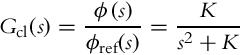
from where closed-loop transfer function of the controlled system can be obtained:
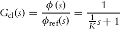
with ϕ(s) and ϕref(s) being the Laplace transforms of φ(t) and φref(t), respectively. The transfer function Gcl(s) is of the first order, which means that in the case of a constant reference the orientation exponentially approaches the reference (with time constant ![]() ). The closed-loop transfer function also has unity gain, so there is no orientation error in steady state.
). The closed-loop transfer function also has unity gain, so there is no orientation error in steady state.
It has been shown that the controller (3.3) made the closed-loop transfer function behave as the first-order system. Sometimes the second-order transfer function ![]() is desired because it gives more degrees of freedom to the designer in terms of the transients shape. We begin the construction by setting the angular acceleration
is desired because it gives more degrees of freedom to the designer in terms of the transients shape. We begin the construction by setting the angular acceleration ![]() of the platform proportional to the robot orientation error:
of the platform proportional to the robot orientation error:
The obtained controlled system
with the transfer function
is the second-order system with natural frequency ![]() and damping coefficient ζ = 0. Such a system is marginally stable and its oscillating responses are unacceptable. Damping is achieved by the inclusion of an additional term to the controller (3.3):
and damping coefficient ζ = 0. Such a system is marginally stable and its oscillating responses are unacceptable. Damping is achieved by the inclusion of an additional term to the controller (3.3):
where K1 and K2 are arbitrary positive control gains. Combining Eqs. (3.1), (3.4) the closed-loop transfer function becomes,
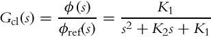
where natural frequency is ![]() , damping coefficient
, damping coefficient ![]() , and closed-loop poles
, and closed-loop poles ![]() .
.
Orientation Control for the Ackermann Drive
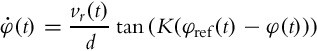
Controller design in the case of the Ackermann drive is very similar to the differential drive controller design; the only difference is due to a different kinematic model (2.19) for orientation that reads

The control variable is α, which can again be chosen proportionally to the orientation error:
The dynamics of the orientation error can be described by the following differential equation obtained by combining Eqs. (3.5), (3.6):
The system is therefore nonlinear. For small angles α(t) and a constant velocity of the rear wheels vr(t) = V, a linear model approximation is obtained,

which can be converted to the transfer function form:

Similarly as in the case of differential drive, the orientation error converges to 0 exponentially (for constant reference orientation) and the decay time constant is ![]() .
.
If the desired transfer function of the orientation feedback loop is of the second order, we follow a similar approach as in the case of the differential drive. Control law given by Eq. (3.4) can be adapted to the Ackermann drive as well:
Assuming again a constant velocity vr(t) = V and small angles α, a linear approximation of Eq. (3.5) is obtained:

Deriving α(t) from Eq. (3.8) and introducing it into Eq. (3.7) yields
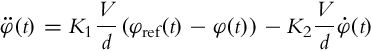
The closed-loop transfer function therefore becomes

The obtained response of the robot orientation is damped with the damping coefficient ![]() and has a natural frequency
and has a natural frequency ![]() .
.
3.2.2 Forward-Motion Control
By forward-motion control we refer to control algorithms that define the translational velocity of the mobile robot v(t) to achieve some control goal. Forward-motion control per se cannot be used as a mobile robot control strategy. For example, if the desired orientation can be achieved by orientation control taking the angular velocity ω(t) as a control in the case of the differential drive, forward-motion control alone cannot drive the robot to a desired position unless the robot is directed to its goal initially. This means that forward-motion control is inevitably interconnected with orientation control.
Nevertheless, the translational velocity has to be controlled to achieve the control goal. In the case of trajectory tracking, the velocity is more or less governed by the trajectory while in the reference pose control the velocity should decrease when we approach the final goal. A reasonable idea is to apply the control that is proportional to the distance to the reference point (xref(t), yref(t)):
Note that the reference position can be constant or it can change according to some reference trajectory. The control (3.9) certainly has some limitations and special treatment is needed in case of very large or very small distances to the reference:
• If the distance to the reference point is large, the control command given by Eq. (3.9) also becomes large. It is advisable to introduce some limitations on the maximum velocity command. In practice the limitations are dictated by actuator limitations, driving surface conditions, path curvature, etc.
• If the distance to the reference point is very small, the robot can in practice “overtake” the reference point (due to noise or imperfect model of the vehicle). As the robot is moving away from the reference point, the distance is increasing, and the robot is accelerating according to Eq. (3.9), which is a problem that will be dealt with when the forward-motion controllers are combined with orientation controllers.
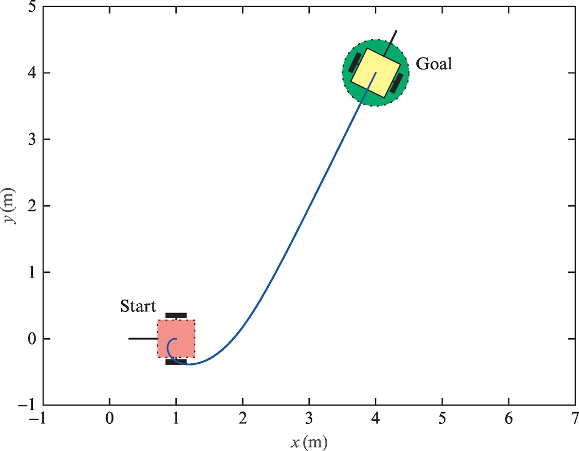
Velocity is inseparably related to acceleration. The latter is also limited in any practical implementation due to the limited forces and torques exerted by the actuators. This aspect is also very important when designing a forward-motion control. One possibility is to limit the acceleration. Usually it is sufficient to just low-pass filter the output of the controller v(t) before the command is sent to the robot in the form of the signal v*(t). The simplest filter of the first order with the DC gain of 1 can be used for this purpose. It is given by a differential equation:
or equivalently with a transfer function
where τf is a time constant of the filter.
In Example 3.1 a simple control algorithm is implemented to drive the robot with Ackermann drive to the reference point. The algorithm contains orientation control and forward-motion control presented previously.
Example 3.1
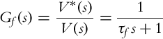
Write a control algorithm for a tricycle robot with a rear-powered pair of wheels to achieve the reference position xref = 4 m and yref = 4 m. The vehicle is controlled with the front-wheel steering angle α and by the rear wheels’ velocity vr. The distance between the front wheel axis and the rear wheels axis is d = 0.1 m. The initial pose of the vehicle is [x(0), y(0), φ(0)] = [1 m, 0, −π]. The control algorithm should consider the vehicle constraints ![]() m/s and
m/s and ![]() .
.
Write a control algorithm and test it on a simulation of the vehicle kinematics using the Euler integration method.
Solution
The orientation control and forward-motion control presented in this section can be used simultaneously. An implementation of solution in Matlab is given in Listing 3.1. Simulation results are shown in Figs. 3.1 and 3.2. It is seen that the vehicle reaches the reference point and stops there. In Fig. 3.2 the control variables are limited according to the vehicle’s physical constraints.

Example 3.2
The same problem as in Example 3.1 has to be solved for the differential drive with a maximum vehicle velocity of ![]() m/s.
m/s.
3.2.3 Basic Approaches
This section introduces several practical approaches for controlling a wheeled mobile robot to the reference pose. They combine the previously introduced orientation and forward-motion control (Sections 3.2.1 and 3.2.2) in different ways and are applicable to wheeled mobile robots that need to achieve a reference pose. They will be illustrated on a differential drive robot but can also be adapted to other wheeled robot types as illustrated previously.
Control to Reference Position
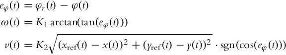
In this case the robot is required to arrive at a reference (final) position where the final orientation is not prescribed, so it can be arbitrary. In order to arrive to the reference point, the robot’s orientation is controlled continuously in the direction of the reference point. This direction is denoted by φr (see Fig. 3.3), which can be obtained easily using geometrical relations:
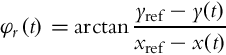
Angular velocity control ω(t) is therefore commanded as
where K1 is a positive controller gain. The basic control principle is similar as in Example 3.1 and is illustrated in Fig. 3.3.
Translational robot velocity is first commanded as proposed by Eq. (3.9):
We have already mentioned that the maximum velocity should be limited in the starting phase due to many practical constraints. Specifically, velocity and acceleration limits should be taken into account.
The control law (3.12) also hides a potential danger when the robot approaches the target pose. The velocity command (3.12) is always positive, and when decelerating toward the final position the robot can accidentally drive over it. The problem is that after crossing the reference pose the velocity command will start increasing because the distance between the robot and the reference starts increasing. The other problem is that crossing the reference also makes the reference orientation opposite, which leads to fast rotation of the robot. Some simple solutions to this problem exist:
• When the robot drives over the reference point, the orientation error abruptly changes (± 180 degrees). The algorithm will therefore check if the absolute value of orientation error exceeds 90 degree. The orientation error will then be either increased or decreased by 180 degree (so that it is in the interval [−180 degree, 180 degree]) before it enters the controller. Moreover, the control output (3.12) changes its sign in this case. The mentioned problems are therefore circumvented by an upgraded versions of control laws (3.11), (3.12):
• When the robot reaches a certain neighborhood of the reference point, the approach phase is finished and zero velocity commands are sent. This mechanism to fully stop the vehicle needs to be implemented even in the case of the modified control law (3.13), especially in case of noisy measurements.
Control to Reference Pose Using an Intermediate Point
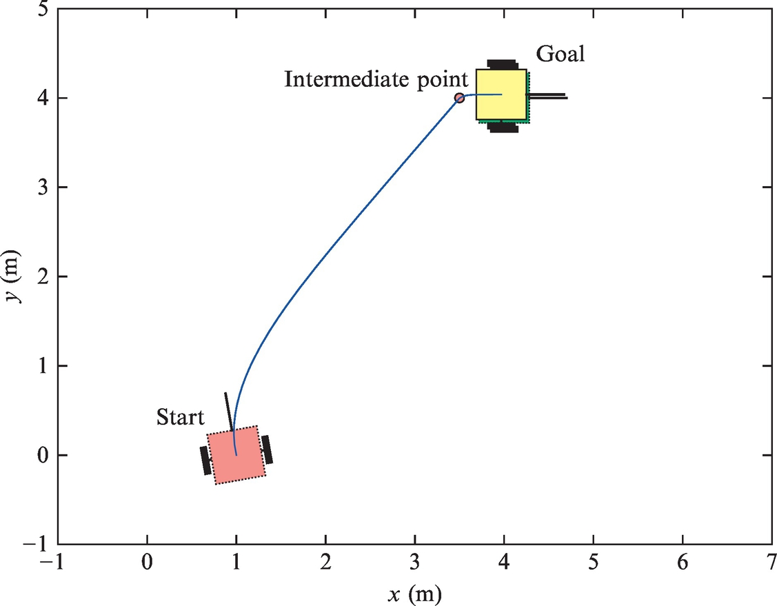
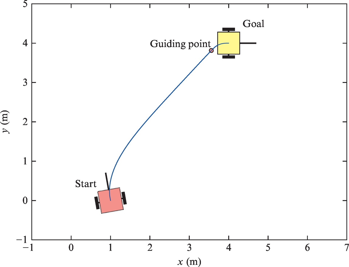
This control algorithm is easy to implement because we use a simple controller given by Eqs. (3.11), (3.12), which drives the robot to the desired reference point. But in this case not only the reference point (xref(t), yref(t)) but also the reference orientation φref is required in the reference point. The idea of this approach is to add an intermediate point that will shape the trajectory in a way that the correct final orientation is obtained. The intermediate point (xt, yt) is placed on the distance r from the reference point such that the direction from the intermediate point toward the reference point coincides with the reference orientation (as shown in Fig. 3.4).

The intermediate point is determined by

The control algorithm consists of two phases. In the first phase the robot is driven toward the intermediate point. When the distance to the intermediate point becomes sufficiently low (checked by condition ![]() ), the algorithm switches to the second phase where the robot is controlled to the reference point. This procedure ensures that the robot arrives to the reference position with the required orientation (a very small orientation error is possible in the reference pose). It is possible to make many variations of this algorithm and also make more intermediate points to improve the operation.
), the algorithm switches to the second phase where the robot is controlled to the reference point. This procedure ensures that the robot arrives to the reference position with the required orientation (a very small orientation error is possible in the reference pose). It is possible to make many variations of this algorithm and also make more intermediate points to improve the operation.
The described algorithm is very simple and applicable in many areas of use. According to the application, appropriate selection of parameters r and dtol should be made.
Example 3.3
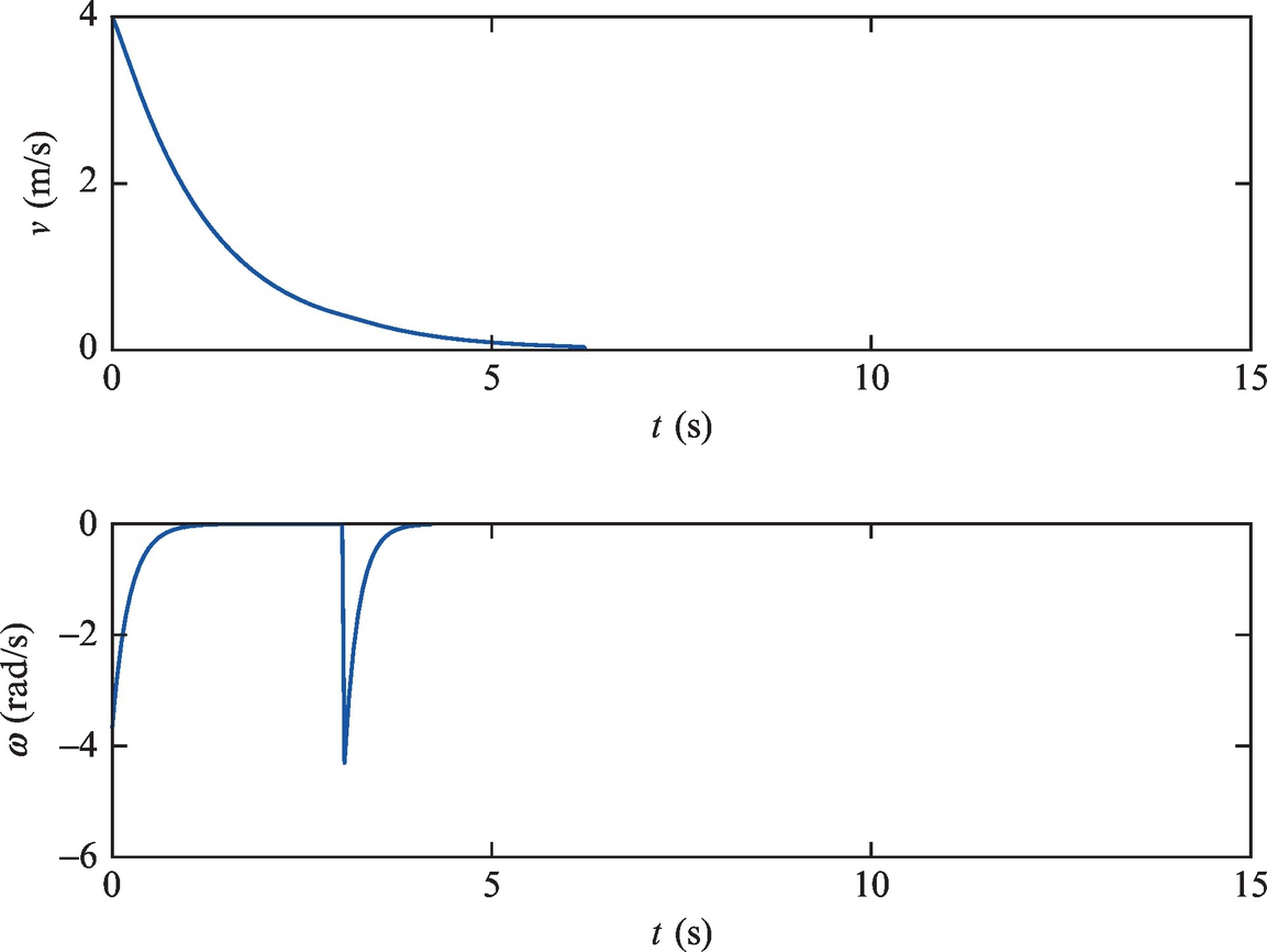
Write a control algorithm for a differential type robot to achieve the reference pose [xref, yref, φref] = [4 m, 4 m, 0 degree] using an intermediate point. Find appropriate values for parameters r and dtol. The initial pose of the vehicle is [x(0), y(0), φ(0)] = [1 m, 0 m, 100 degree].
Test the control algorithm by means of simulation of the differential drive vehicle kinematics.
Solution
M-script code of a possible solution is given in Listing 3.2. Simulation results are shown in Figs. 3.5 and 3.6.
Control to Reference Pose Using an Intermediate Direction
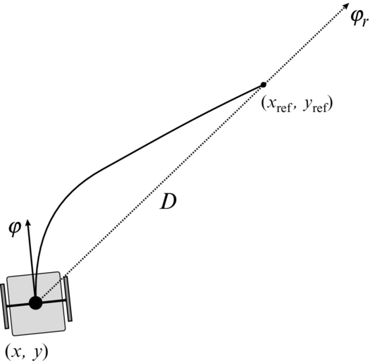
A robot needs to arrive from its initial pose to the reference pose where the position (xref, yref) and the orientation φref are given. The idea of the algorithm with an intermediate direction is illustrated in Fig. 3.7 [2]. We begin with the construction of a right-angled triangle. The reference point is put to the vertex with the right angle. One cathetus connects the current robot position with the reference one and has the length ![]() . This cathetus defines the orientation φr that is facing from the robot toward the target. The other cathetus has a fixed length of r > 0, which is a designer parameter of this method. The angle between cathetus D and the hypotenuse is denoted by β(t). Two angles play a crucial role in this approach, and they are defined as follows:
. This cathetus defines the orientation φr that is facing from the robot toward the target. The other cathetus has a fixed length of r > 0, which is a designer parameter of this method. The angle between cathetus D and the hypotenuse is denoted by β(t). Two angles play a crucial role in this approach, and they are defined as follows:

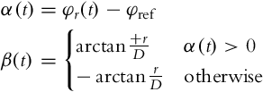
Note that the angles α(t) and β(t) are always of the same sign (in the case depicted in Fig. 3.7 they are both positive). If α becomes 0 at a certain time, β becomes irrelevant, so its sign can be arbitrary. Large values (in the absolute sense) of α mean that driving straight to the reference is not a good idea because the orientation error will be large in the reference pose. The angle α should therefore be reduced (in the absolute sense). This is achieved by defining an intermediate direction that is shifted from φr, and the shift is always away from the reference orientation φref (if the reference orientation is seen pointing to the right from the robot’s perspective, the robot should approach the reference position from the left side, and vice versa). While α(t) normally decreases (in the absolute sense) when approaching the target, β(t) increases (in the absolute sense) as the distance to the reference decreases. We will make use of this when constructing the control algorithm.
The algorithm again has two phases. In the first phase (when |α(t)| is large), the robot’s orientation is controlled toward the intermediate direction φt(t) = φr(t) + β(t) (this case is depicted in Fig. 3.7). When the angles α and β become the same, the current reference orientation switches to φt(t) = φr(t) + α(t). Note that this switch does not cause any bump because both directions are the same at the time of the switch. The control law for orientation is therefore defined as follows:
Note that the current reference heading is never toward the reference point but is always slightly shifted. The shift is chosen so that the angle α(t) is driven toward 0. This in turn implies that the reference heading is forced toward the reference point and the robot will arrive there with the correct reference orientation. Note that this algorithm is also valid for negative values of angles α and β. We only need to ensure that all the angles are in the (−π, π] interval.
Robot translational velocity can be defined similarly as in the previous sections.
Example 3.4
Write a control algorithm for a differential type robot to achieve the reference pose [xref, yref, φref] = [4 m, 4 m, 0 degree] using the presented control to the reference pose using an intermediate direction. Find an appropriate value for parameter r. The initial pose of the vehicle is [x(0), y(0), φ(0)] = [1 m, 0 m, 100 degree]. Test the algorithm on a simulated kinematic model.
Solution
The M-script code of a possible solution is in Listing 3.3. Simulation results are shown in Figs. 3.8 and 3.9.

Control on a Segmented Continuous Path Determined by a Line and a Circle Arc
The path composed from straight line segments and circular arcs is known to be the shortest possible path for Ackermann drive robots as shown in [3–5], where the circle’s radius is the minimal turning radius of the vehicle. Such a path is also the shortest possible for a differential robot where the minimum circle radius limits to zero, which means that the robot can turn on the spot.
The basic idea of the algorithm can be described with the illustration in Fig. 3.10. First, a circle of an appropriate (this will be discussed later) radius R is drawn through the reference point tangentially to the reference orientation. Note that two solutions exist, and a circle whose center is closer to the robot is chosen. This circle, more precisely a certain arc belonging to this circle, represents the second part of the planned path. The first part will run on a straight line tangent to the circle and crossing the current robot’s position. Again, two tangents exist, and we select the one that gives proper direction of driving along the circular arc. The direction of driving along the arc is defined with the reference orientation (in the case illustrated in Fig. 3.10 the robot will drive along the circle in the clockwise direction). The solution can be chosen easily by checking the sign of the cross products between the radius vectors and the tangential vectors.

In the first part of the algorithm the goal is to drive toward the point (xt, yt) where the straight segment meets the arc segment. The orientation controller is a very simple one:
where ![]() . When the distance to the intermediate point is small enough, the second phase begins. This includes driving along the trajectory, and the controller changes to
. When the distance to the intermediate point is small enough, the second phase begins. This includes driving along the trajectory, and the controller changes to
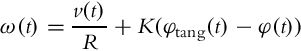
where R is the circle radius, v(t) is the desired translational velocity, and φtang(t) is the direction of the tangent to the arc in the current robot position. Note that the first term in the control is a feedforward part that ensures the robot will drive along the circular arc with radius R, while the second term is a feedback control that corrects the control errors.
To achieve higher robustness the reference path is calculated in each iteration, which ensures that the robot is always on the reference straight line or on the reference circle. The obtained path slightly differs from the ideal one composed of a straight line segment and a circular arc. The mentioned difference is due to inial robot orientation that does not coincide with the constructed tangent. Other reasons for this difference are noise and disturbances (wheels slipping and the like).
This reference path is relatively easy to determine in real time. The path itself is continuous, but the required inputs are not. Due to transition from the straight line to the circle the robot angular velocity instantly changes from zero to ![]() . In reality this is not achievable (limited robot acceleration), and therefore some tracking error appears in this transition.
. In reality this is not achievable (limited robot acceleration), and therefore some tracking error appears in this transition.
Such a control is appropriate for situations where a robot needs to arrive to the reference pose quickly and the shape of the path is not prescribed but the length should be as short as possible (e.g., robot soccer). Especially if we deal with the robots with a limited turning radius (e.g., Ackermann drive), such a path is the shortest possible to the goal pose if the minimal robot turning radius is used for parameter R. But of course, this leads to high values of radial accelerations, so perhaps a larger value of R is desired.
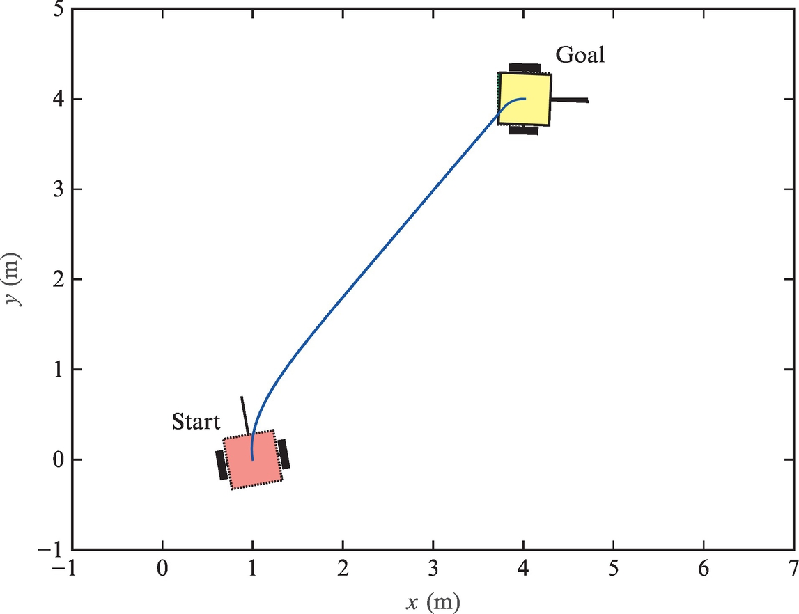
Example 3.5
Write a control algorithm for a differential type robot to achieve the reference pose [xref, yref, φref] = [0 m, 0 m, 0 degree] using the control algorithm proposed in this section. The radius of the circle should be R = 0.4 m. The initial pose of the vehicle is [x(0), y(0), φ(0)] = [−3 m, −3 m, 100 degree]. Test the algorithm on a simulated kinematic model.
Solution
Although the basic idea of the control algorithm is quite simple, the implementation becomes a bit more complicated as it needs to calculate appropriate circle centers, tangent points on the circle, and some other parameters. A possible solution is given in Listing 3.4, and the simulation results are shown in Figs. 3.11 and 3.12.

From Reference Pose Control to Reference Path Control
Often the control goal is given with a sequence of reference points that a robot should drive through. In these cases we no longer speak about reference pose control but rather a reference path is constructed through these points. Often straight line segments are used between the individual points, and the control goal is to get to each reference point with the proper orientation, and then automatically switch to the next reference point. This approach is easy to implement and usually sufficient for use in practice. Its drawback is the nonsmooth transition between neighboring line segments, which causes jumps of control error in these discontinuities.
The path is defined by a sequence of points Ti = [xi, yi]T, where i ∈ 1, 2, …, n, and n is the number of points. In the beginning the robot should follow the first line segment (between points T1 and T2), and it should arrive to T2 with orientation defined by the vector ![]() . When it reaches the end of this segment it starts to follow the next line segment (between the points T2 and T3), and so on. Fig. 3.13 shows actual line segment between points Ti and Ti+1 with variables marked. Vector v =Ti+1 −Ti = [Δx, Δy]T defines the segment direction, and vector r = R −Ti is the direction from point Ti to the robot center R. The vector vn = [Δy, −Δx] is orthogonal to the vector v.
. When it reaches the end of this segment it starts to follow the next line segment (between the points T2 and T3), and so on. Fig. 3.13 shows actual line segment between points Ti and Ti+1 with variables marked. Vector v =Ti+1 −Ti = [Δx, Δy]T defines the segment direction, and vector r = R −Ti is the direction from point Ti to the robot center R. The vector vn = [Δy, −Δx] is orthogonal to the vector v.
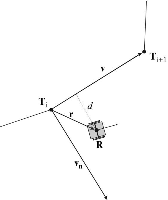
The robot must follow the current line segment while the projection of vector r to vector v is inside the interval defined by points Ti in Ti+1. This condition can be expressed as follows:
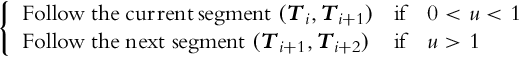
where u is the dot product

Variable u is used to check if the current line segment is still valid or the switch to the next line segment is necessary.
Orthogonal distance of the robot from the line segment is defined using the normal vector vn:
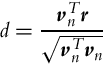
If we normalize distance d by the distance length we obtain normalized orthogonal distance dn between the robot and the straight line:

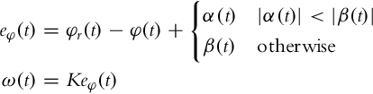
Normal distance dn is zero if the robot is on the line segment and is positive if the robot is on the right side of the segment (according to vector v) and vice versa. Normal distance dn is used to define desired direction or robot motion. If the robot is on the line segment or very close to it then it needs to follow the line segment. If, however, the robot is far away from the line segment then it needs to drive perpendicularly to line segment in order to reach the segment faster. The reference orientation of driving in a certain moment can be defined as follows:
where φlin = arctan2(Δy, Δx) (note that the function arctan2 is the four-quadrant inverse tangent function) is the orientation of the line segment and ![]() is an additional reference rotation correction that enables the robot to reach the line segment. Gain K1 changes the sensitivity of φrot according to dn. Because φref is obtained by addition of two angles it needs to be checked to be in the valid range [−π, π].
is an additional reference rotation correction that enables the robot to reach the line segment. Gain K1 changes the sensitivity of φrot according to dn. Because φref is obtained by addition of two angles it needs to be checked to be in the valid range [−π, π].
So far we define a reference orientation that the robot needs to follow using some control law. The control error is defined as
where φ is the robot orientation. From orientation error the robot’s angular velocity is calculated using a proportional controller:
where K2 is a proportional gain. Similarly, also a PID controller can be implemented, where the integral part speeds up the decay of eφ while the differential part damps oscillations due to the integral part. Translational robot velocity can be controlled by basic approaches discussed in the preceding sections.
Example 3.6
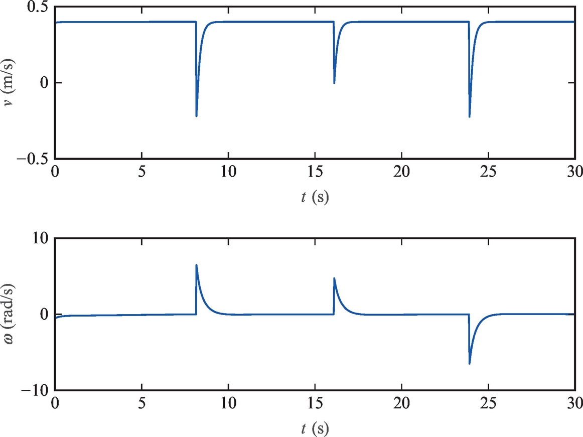
Write a control algorithm for a differentially driven robot to drive on the sequence of line segments defined by points T1 = [3, 0], T2 = [6, 4], T3 = [3, 4], T4 = [3, 1], and T5 = [0, 3]. Find appropriate values for parameters K1 and K2. The initial pose of the vehicle is [x(0), y(0), φ(0)] = [5 m, 1 m, 108 degree]. Test the algorithm on a simulated kinematic model.
Solution
An M-script code of a possible solution is given in Listing 3.5. The reference path and the actual robot motion curve are shown in Fig. 3.14, and the control signals are shown in Fig. 3.15.

Try to extend the code given in the solution so that the robot could also drive in reverse if ![]() .
.
3.3 Trajectory Tracking Control
In mobile robotics, a path is a “line” that a robot needs to drive in the generalized coordinates space. If a path is parameterized with time, that is, motion along the path has to be synchronized with time, then we speak about a trajectory. Whenever the schedule of a robot motion is known in advance, the (reference) trajectory of the robot can be written as a time-function in the generalized coordinate’s space: ![]() . For practical reasons, the trajectory is always defined on a finite time interval t ∈ [0, T], that is, the reference trajectory has a start point and an end point. Trajectory tracking control is a mechanism that will ensure the robot trajectory q(t) is as close as possible to the reference one qref(t) despite any difficulties encountered.
. For practical reasons, the trajectory is always defined on a finite time interval t ∈ [0, T], that is, the reference trajectory has a start point and an end point. Trajectory tracking control is a mechanism that will ensure the robot trajectory q(t) is as close as possible to the reference one qref(t) despite any difficulties encountered.
3.3.1 Trajectory Tracking Control Using Basic Approaches
When thinking of implementing a trajectory tracking control, the first idea would probably be to imagine the reference trajectory as a moving reference position. Then in each sampling time of the controller, the reference point moves to the current point of the reference trajectory (xref(t), yref(t)), and the control to the reference position is applied via control laws (3.11), (3.12). Note that here the robot is required to drive as closely as possible to this imaginary reference point. When the velocity is low and the position measurement is noisy, the robot position measurement can be found ahead of the trajectory. It is therefore extremely important to handle such situations properly, for example, by using an updated control law (3.13).
This approach suffers from the fact that feedback carries the main burden here and relatively large control gains are needed in order to make the control errors small. This makes the approach susceptible to disturbances in the control loop. It is therefore advantageous to use feedforward compensation that will be introduced in Section 3.3.2.
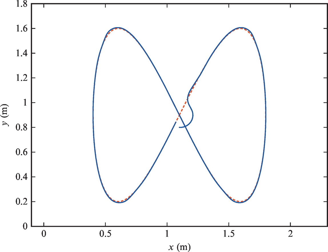
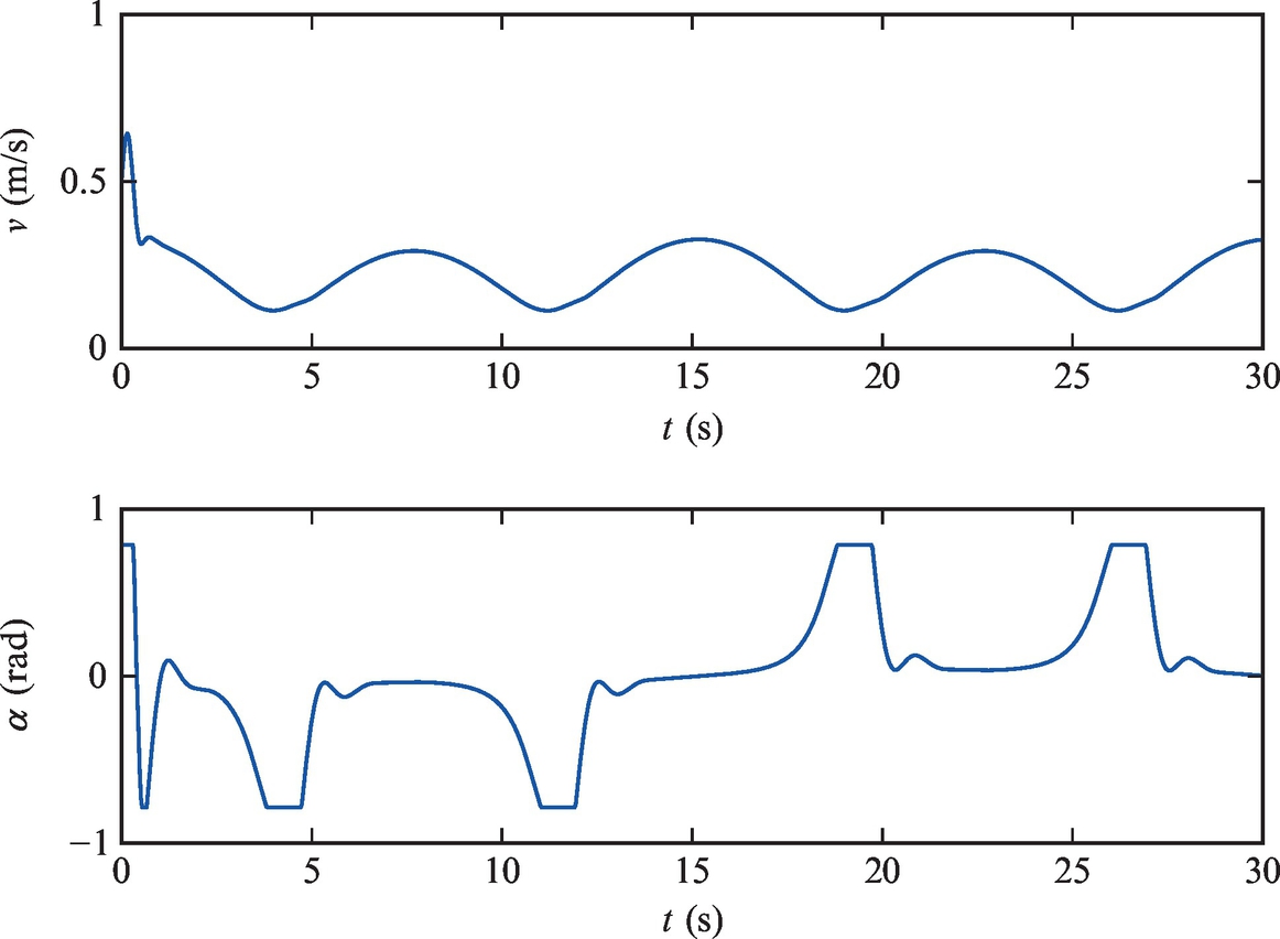
Example 3.7
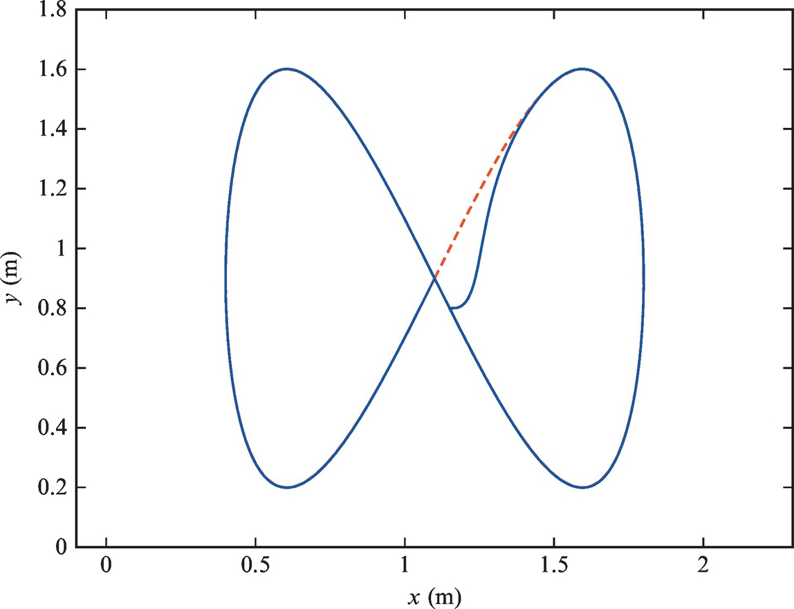
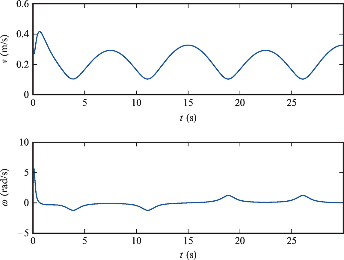
A tricycle robot with a rear-powered pair of wheels from Example 3.1 has to be controlled to follow the reference trajectory ![]() and
and ![]() . The initial pose of the vehicle is [x(0), y(0), φ(0)] = [1.1, 0.8, 0]. Write two control algorithms and test them on a simulated kinematic model:
. The initial pose of the vehicle is [x(0), y(0), φ(0)] = [1.1, 0.8, 0]. Write two control algorithms and test them on a simulated kinematic model:
• The first approach uses the basic control laws (3.11), (3.12).
• The second approach uses the upgraded control law (3.13).
Solution
By changing the value of the variable UpgradedLaw the control can switch between the so-called basic one, given by Eqs. (3.11), (3.12), and the upgraded one given by Eq. (3.13). The results of Example 3.7 are shown in Figs. 3.16 and 3.17 (in the tested case the basic and the upgraded control law behave the same).
The Matlab code is given in Listing 3.6.
3.3.2 Decomposing Control to Feedforward and Feedback Action
Trajectory tracking control is significant not only from a practical point of view, but also from a theoretical point of view. Its importance stems from the famous result that according to Brockett’s condition nonholonomic systems cannot be asymptotically stabilized around the equilibrium using smooth time-invariant feedback [1]. This result can be checked easily for the case of the differential drive, and it can be extended to other kinematics including Ackermann kinematics. First, we start by checking whether the system is driftless. Since the derivative of the vector field ![]() is zero in the case of no control (v = 0, ω = 0), the system is indeed driftless. Brockett [1] showed that one of the conditions for a driftless system to be stabilized by a continuous time-invariant feedback is that the number of inputs should be at least the same as the number of states. In the case of the differential drive this condition is clearly violated and other types of feedback should be sought. Nevertheless, completely nonholonomic, driftless systems are still controllable in a nonlinear sense. Therefore, asymptotic stabilization can be obtained using time-varying, discontinuous, or hybrid control laws. One of the possibilities to circumvent the limitation imposed by Brockett’s condition is to introduce a different control structure. In the case of trajectory tracking control very often a two-degree-of-freedom control is used where one path corresponds to the feedforward path and the other corresponds to the feedback path from the control system’s terminology.
is zero in the case of no control (v = 0, ω = 0), the system is indeed driftless. Brockett [1] showed that one of the conditions for a driftless system to be stabilized by a continuous time-invariant feedback is that the number of inputs should be at least the same as the number of states. In the case of the differential drive this condition is clearly violated and other types of feedback should be sought. Nevertheless, completely nonholonomic, driftless systems are still controllable in a nonlinear sense. Therefore, asymptotic stabilization can be obtained using time-varying, discontinuous, or hybrid control laws. One of the possibilities to circumvent the limitation imposed by Brockett’s condition is to introduce a different control structure. In the case of trajectory tracking control very often a two-degree-of-freedom control is used where one path corresponds to the feedforward path and the other corresponds to the feedback path from the control system’s terminology.
Before introducing feedforward and feedback control, we need to define another important system property. A system is called differentially flat if there exist a set of flat outputs, and all the system states and system inputs can be rewritten as functions of these flat outputs and a finite number of their time derivatives. This means that some nonlinear functions fx and fu have to exist satisfying

where vectors x, u, and zf represent the system states, its inputs, and flat outputs, respectively, while p is a finite integer. We should also mention that flat outputs should be functions of system states, its inputs, and a finite number of input derivatives. This means that in general flat outputs are fictitious; they do not correspond to the actual outputs.
In case of the differential drive kinematic model given by Eq. (2.2) the flat outputs are actual system outputs x and y. It can easily be shown that all the inputs (both velocities) and the third state (robot orientation) can be represented as functions of x and y, and their derivatives. We know that ![]() and
and ![]() can be interpreted as Cartesian coordinates of the robot’s translational velocity. Therefore, the translational velocity is obtained by the Pythagorean sum of its component:
can be interpreted as Cartesian coordinates of the robot’s translational velocity. Therefore, the translational velocity is obtained by the Pythagorean sum of its component:
Due to nonholonomic constraints, a differentially driven wheeled robot always moves in the direction of its orientation, which means that the tangent of the orientation equals the quotient of Cartesian components of the translational velocity:

Finally, angular velocity ω(t) is determined as the time derivative of the orientation φ(t) given by Eq. (3.17)
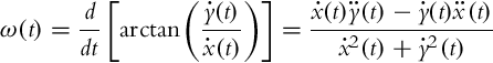
and is not defined only if the translational velocity becomes 0.
Cartesian coordinates of the position x and y are also the flat outputs of the rear-wheel-powered bicycle kinematic model given by Eq. (2.19). The first two equations of this kinematic model are the same as in the case of the differential drive equation (2.2), and therefore the velocity of the rear wheel and the orientation can be obtained by expressions in Eqs. (3.16), (3.17). The third equation in Eq. (2.19) is
from where it follows
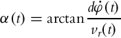
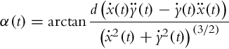
The input α(t) can be rewritten by flat outputs and their derivatives by introducing the expressions in Eqs. (3.16), (3.18) into Eq. (3.20) instead of vr(t) and ![]() :
:
A very important consequence of the above analysis is that the Ackermann drive is structurally equivalent to the differential drive. To illustrate this, if a certain command {v(t), ω(t)} is applied to a differentially driven robot, the obtained trajectory is the same as if a command ![]() is applied to the robot with Ackermann drive. A large majority of the examples that follow are performed on a differentially driven robot. Those results can therefore be easily extended to robots with Ackermann drive and to some other kinematic structures as well.
is applied to the robot with Ackermann drive. A large majority of the examples that follow are performed on a differentially driven robot. Those results can therefore be easily extended to robots with Ackermann drive and to some other kinematic structures as well.
If the system is flat, then all the system variables can be deduced from flat outputs without integration. A useful consequence of this fact is that based on the reference trajectory, the required control inputs can be calculated analytically. In the case of a differentially driven wheeled robot, Eqs. (3.16), (3.18) provide formulae for obtaining reference velocities vref(t) and ωref(t) from the reference trajectory given by xref(t) and yref(t):

Note that similar formulae can also be obtained for other kinematic structures associated with flat systems.
Eqs. (3.22), (3.23) provide open-loop controls that ensure that the robot drives along the reference trajectory in the ideal case where the kinematic model of the robot exactly describes the motion, and there are no disturbances, measurement errors, and initial pose error. These assumptions are never met completely, and some feedback control is necessary. In these cases the reference velocities from Eqs. (3.22), (3.23) are used in the feedforward part of the control law while a wide spectrum of possible feedback control laws can be used. Some of them will also be discussed in the following sections.
3.3.3 Feedback Linearization
The idea of feedback linearization is to introduce some transformation (usually to the system input) that makes the system between new input and output linear. Thus any linear control design is made possible. First, we have to make sure that the system is differentially flat [6, 7]. We have shown in Section 3.3.2 that many kinematic structures are flat. Then, the procedure of designing a feedback linearization is as follows:
• The appropriate flat outputs should be chosen. Their number is the same as the number of the system inputs.
• Flat outputs should be differentiated and the obtained derivatives checked for the functional presence of inputs. This step is repeated until all the inputs (or their derivatives) appear in the flat output derivatives. If all the inputs (more precisely their highest derivatives) can be derived from this system of equations, we can proceed to the next step.
• The system of equations is solved for the highest derivatives of individual inputs. To obtain actual system inputs, a chain of integrators has to be used on the input derivatives. The output derivatives, on the other hand, serve as new inputs to the system.
• Since the newly obtained system is linear, a wide selection of possible control laws can be used on these new inputs.
In the case of a wheeled mobile robot with differential drive, the flat outputs are x(t) and y(t). Their first derivative according to the kinematic model (2.2) is
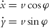
In the first derivatives, only the translational velocity v appears, and the differentiation continues:
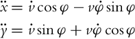
In the second derivatives both velocities (v and ![]() ) are present. Now the system of equations is rewritten so that the second derivatives of the flat outputs are described as functions of the highest derivatives of individual inputs (
) are present. Now the system of equations is rewritten so that the second derivatives of the flat outputs are described as functions of the highest derivatives of individual inputs (![]() and ω in this case):
and ω in this case):
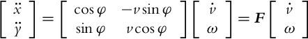
The matrix F has been introduced, which is nonsingular if v≠0. The system of equations can therefore be solved for ![]() and ω:
and ω:
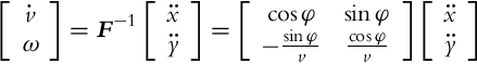
The solution ω from Eq. (3.25) is the actual input to the robot, while the solution ![]() should be integrated before it can be used as an input. The newly obtained linear system has inputs
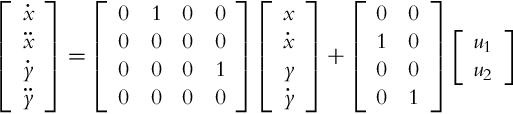
should be integrated before it can be used as an input. The newly obtained linear system has inputs ![]() , and the states
, and the states ![]() (the kinematic model (2.2) has three states; the fourth one is due to an additional integrator). The dynamics of the new system can be described conveniently by the state-space representation:
(the kinematic model (2.2) has three states; the fourth one is due to an additional integrator). The dynamics of the new system can be described conveniently by the state-space representation:
or in a compact form as
The system (3.27) is controllable because its controllability matrix,
has full rank, and therefore the state controller exists for an arbitrarily chosen characteristic polynomial of the closed loop. An additional requirement is to design the control law so the robot will follow a reference trajectory. In the context of flat systems, a reference trajectory is given for the flat outputs, in this case xref(t) and yref(t). Then the reference can easily be obtained for the system state ![]() and the system input
and the system input ![]() . Eq. (3.27) can also be written for the reference signals:
. Eq. (3.27) can also be written for the reference signals:
The error between the actual states and the reference states is defined as ![]() . Subtracting Eq. (3.29) from Eq. (3.27) yields
. Subtracting Eq. (3.29) from Eq. (3.27) yields
Eq. (3.30) describes the dynamics of the state error. These dynamics should be stable and appropriately fast. One way to prescribe the closed-loop dynamics is to require specific closed-loop poles. We have already shown that the pair (A, B) is a controllable one, and therefore by properly selecting a constant control gain matrix K (of dimension 2 × 4), arbitrary locations of the closed-loop poles in the left half-plane of the complex plane s can be achieved. Eq. (3.30) can be rewritten:
If the last term in Eq. (3.31) is zero, the state errors converge to 0 with the prescribed dynamics, given by the closed-loop system matrix (A −BK). Forcing this term to 0 defines the control law for this approach:
Schematic representation of the complete control system is given in Fig. 3.18.

Due to a specific form of matrices A and B in Eq. (3.26), where u1 only influences states z1 and z2 while u2 only influences states z3 and z4, the control gain matrix takes a special form:

The control law (3.32) can therefore be completely decomposed:
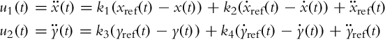
The proposed approach requires that all the states are known. While x and y are usually measured, their derivatives are not. Numerical differentiation amplifies noise and should be avoided in practice. Two possible solutions are as follows:
• The unmeasured states can be estimated by state observers.
• If the robot orientation φ is measured, the derivatives can be calculated as ![]() ,
, ![]() .
.
A practical example of this approach is shown in Example 3.8.
Example 3.8
A differentially driven vehicle is to be controlled to follow the reference trajectory ![]() and
and ![]() . The sampling time is Ts = 0.033 s. The initial pose is [x(0), y(0), φ(0)] = [1.1, 0.8, 0]. Implement the algorithm presented in this section in a Matlab code and show the graphical results.
. The sampling time is Ts = 0.033 s. The initial pose is [x(0), y(0), φ(0)] = [1.1, 0.8, 0]. Implement the algorithm presented in this section in a Matlab code and show the graphical results.
Solution
The code is shown in Listing 3.7. The results of Example 3.8 are shown in Figs. 3.19 and 3.20. In this approach the problems of periodic orientation do not appear (there is no need to map angles to the (−π, π] interval). This stems from the fact that the orientation always appears within trigonometric functions that are periodic by themselves.