Keywords

Evaluation of localization systems; fingerprinting; Fisher information; multilateration; packet radio localization; pedestrian dead reckoning (PDR); range-based localization; range-free localization; received signal strength (RSS) indicator; simultaneous localization and mapping (SLAM)

1 Introduction

Localization of devices and people has been recognized as one of the main building blocks of context aware systems [1–4], which have one of their main application fields in ambient assisted living (AAL). Indeed, the user position can be used for detecting user activities, activating devices, opening doors, etc. While in outdoor scenarios GNSS (global navigation satellite systems) constitute a reliable and easily available technology, in indoor scenarios GNSS is largely unavailable.

The indoor environment lacks a system that possesses the excellent performance parameters of outdoor GNSS in terms of global coverage, high accuracy, short latency, high availability, high integrity, and low user costs. Like indoor settings, certain outdoor environments are not well covered by GNSS due to insufficient views to the open sky.

Therefore, the indoor localization problem is solved by means of ad hoc solutions, among which one of the most promising is based on wearable technologies. Improvements in indoor positioning performance have the potential to create opportunities for businesses. However, system performances differ greatly, because the environments have a number of substantial dissimilarities. Indoor environments are particularly challenging for localization systems for several reasons:

On the other hand, indoor settings facilitate positioning and navigation in many ways:

Indoor localization systems can be classified based on the signal types and/or technologies (infrared, ultrasound, ultra-wideband, RFID, packet radio), signal metrics (AOA – angle of arrival, TOA – time of arrival, TDOA – time difference of arrival, and RSS – received signal strength) and the metric processing methods (range-based and range-free algorithms) [5]. Each solution has advantages and shortcomings, which, in most cases, can be summarized in a trade-off between several metrics (such as accuracy, installation complexity, etc.).

In the following we will discuss which metrics are important for evaluating indoor localization systems, the technologies, and the main localization algorithms (namely, range-free and range-based algorithms).

2 Evaluation Metrics

In order to evaluate the localization systems a set of criteria weighted according to their relevance and importance for a given applications must be defined. The combination of different metrics makes it possible to evaluate the overall performance of a localization system.

EvAAL (Evaluating AAL Systems through Competitive Benchmarking) [6] is an ongoing effort toward establishing benchmarks and evaluation metrics for comparing ambient-assisted living solutions. Each year one or more international competitions are organized, with the long-term goal of evaluating complete AAL systems. In the last three years an international competition on indoor localization has been organized and five metrics identified.

Two of them are objectively measurable (hard) quantities, namely accuracy and availability. Accuracy is the classical measurement of the goodness of a localization system, based on samples of the distance between the point where the system locates the user and the point where the user really is (error distance). The error series should be reduced to a scalar score, and the literature is rich in methods to reach this result. Of the 195 papers of the first edition of the Indoor Positioning and Indoor Navigation (IPIN, 2010) conference, 115 works describe real or simulated systems that are amenable to being evaluated by measuring some kind of metrics. The metrics taken into account in these works are visual path comparison, usually as a graph that shows the real and the estimated path (32% of cases), mean error (31%), cumulative distribution function CDF (20%), a quantile value (11%), and finally error variance (5%).

Availability is a measure of how well the system performs at providing regularly spaced measurements: this is especially significant for experimental or prototypal systems. In other words, the availability measures the capacity of the systems to produce fresh data continuously. As such, it is simply computed as the ratio between the number of received samples and the number of expected samples (one every half a second for the EvAAL competition).

Besides hard quantities, some soft ones need to be considered, namely installation complexity, user acceptance, and interoperability with AAL systems.

Installation complexity is a measure of effort required to install the AAL localization system in a home. It is measured as a function of the person minutes of work needed to complete the installation.

User acceptance expresses how much the localization system is invasive in the user’s daily life and thereby the impact perceived by the user. This parameter is estimated with a simple questionnaire (available on the EvAAL website) that considers aspects of usability like the presence and invasiveness of the tags, the visibility of the installation within the environment, and the complexity of maintenance procedures.

Interoperability measures how much the system is easy to integrate with other systems. This parameter depends on the scenario in which the localization system is evaluated, since localization can be exploited by other applications to offer advanced services. In EvAAL the interoperability is also measured with a questionnaire that takes into account aspects like the availability of APIs and documentation, the licensing scheme, the presence of testing tools, and the portability among different operating systems.

All these metrics must be taken into account to discuss the performance of an indoor localization system. The rationale behind the choice of these metrics is multi-faceted. First of all, the accuracy is the most important metric to assess the performance of a localization and tracking system. In general indoor applications do not need high precision, and giving accuracy too much importance diminishes the significance of the evaluation performance with respect to real-life systems. The availability is also an important metric because an unresponsive system can be as difficult to manage as an inaccurate one. Therefore, the weight to give to the hard metrics together should not be more than the weight of metrics related to interaction with the main stakeholders for a given system: system integrators, installers, and final users.

3 Technologies

Many different technologies are used for localization purposes. Most of them require the user to be localized to wear or carry some sort of device.

If the on-body devices need to communicate or otherwise respond to external (not on-body) devices we speak of on-body active systems. The external devices are typically part of some infrastructure that is deployed in the environment and which is able to track users. Being infrastructure-based, these systems can be arbitrarily powerful: they can interact with other systems in a variety of ways, they can provide user interfaces (e.g., a graphical web interface), and they can carry on sophisticated computations on data received from on-body devices.

If the on-body devices gather information from the environment and interpret it without the need to actively communicate anything or respond to some external device, we speak of on-body passive systems. The information gathered by the on-body system can be generated by some external devices for the purpose of allowing localization, or else can be opportunistically gathered from the environment and the body movements.

Last, we speak about device-free systems where no on-body device is necessary to achieve localization. In this case, as in the case of active systems, an external infrastructure senses the position and movements of the user.

Each of the above categories can use several different technologies, which are treated in the following sections. Currently, no single low-cost method is accurate or general enough to provide satisfactory performance. Practical systems need to fuse information created by more subsystems in order to obtain satisfactory performance at low cost. This topic is treated in the following section.

4 Wearable Radios

Wearable-based solutions estimate the (unknown) location of the mobile sensors (hereafter also called mobiles) with respect to a set of fixed sensors (called anchors), whose position is known. The position estimation of a mobile can be achieved by using two different approaches, either range-based or range-free. The former consists of protocols that use absolute point-to-point distance estimates for calculating the location. The latter makes no assumption about the availability or validity of such information. The effectiveness of these two localization approaches depends on the accuracy required by the applications that use the location information. Acknowledging that the range-free solutions have a coarse accuracy [13], these techniques are unsuitable in applications where location accuracy is one of the main requirements. On the other hand, range-based localization exploits measurements of physical quantities related to beacon packets exchanged between the mobile and the anchors. Radio signal measurements are typically the received signal strength (RSS), the angle of arrival (AOA), the time of arrival (TOA), or the time difference of arrival (TDOA). Although AOA or TDOA can guarantee a high localization precision, they require specific and complex hardware. This is a major drawback in particular in AAL applications, which are deeply involved with users’ monitoring and thus may suffer from complex and invasive hardware.

There are at least two possible scenarios where RSS techniques are suited better than other radio signal measurement techniques. In the first, futuristic scenario, wireless sensors are ubiquitous in the environment and on the user’s body for health monitoring. In this case, no additional equipment is required to localize the user. In the second scenario, various sensors (i.e., gyroscopes, accelerometers, compass, and pressure sensor) are placed on the user’s body to recognize the movements. In the common case of sensors using wireless communications, exploiting the RSS measurements can give an additional source of information (such as the position of the user) at no additional equipment cost. For these reasons in the following sections of this chapter we will refer only to RSS-based localization techniques.

4.1 Range-Free

In this section we present the most used and referenced range-free localization schemes that use radio connectivity to infer proximity to a set of anchor nodes. These schemes make no assumptions about the availability or validity of point-to-point distance estimation.

4.1.1 Centroid

The centroid scheme was proposed in [14]. This localization scheme assumes that a set of anchor nodes (A_i, 1 ≤i ≤ n), with overlapping regions of coverage, exist in the deployment area of the WSN. The main idea is to treat the anchor nodes, located at (X_i, Y_i), as physical points of equal mass and to find the center of gravity (centroid) of all these masses:

$(X_G,Y_G)=\left(\frac{{\sum }_{i=1}^n{X}_i}{n},\frac{{\sum }_{i=1}^n{Y}_i}{n}\right)$ (1)

(1)

An example of how the centroid scheme works is shown in Figure 1, where a sensor node N_k is within communication range to four anchor nodes, A₁…A₄. The node N_k localizes itself to the centroid of the quadrilateral A₁ A₂ A₃ A₄ (for the case of a quadrilateral, the centroid is at the point of intersection of the bimedians – the lines connecting the middle points of opposite sides).

4.1.2 APIT

APIT [15] is an area-based range-free localization scheme. It assumes that a small number of nodes, called anchors, are equipped with high-powered transmitters and know their location, obtained via GPS or some other mechanism. Using beacons from these anchors, APIT employs a novel area-based approach to perform location estimation by marking the environment with triangular regions between anchor nodes as shown in Figure 2. A node’s presence inside or outside of these triangular regions allows a node to narrow down the area in which it can potentially reside. By using different combinations of anchors, the size of the estimated area in which a node resides can be reduced to provide a good location estimate.

The method used to narrow down the possible area in which a target node resides is called the point-in-triangulation test (PIT). For three given anchors, A, B, and C, the PIT chooses whether a point M with an unknown position is inside triangle ABC or not. APIT repeats the PIT with different anchor combinations until all combinations are exhausted or the required accuracy is achieved. At this point, APIT calculates the centroid of the intersection of all of the triangles in which a node resides to find its estimated position. In [16] the authors implemented the APIT system on an outdoor experimental testbed showing that at least 80% of nodes lie within a one-hop region of their estimated areas. Both simulation and experimental results have verified that APIT is a promising technique for range-free localization in large outdoor sensor networks.

4.1.3 SeRLoc

SeRLoc [17] is another area-based range-free localization method. SeRLoc assumes two types of nodes: normal nodes and locators (i.e., anchors). Normal nodes are equipped with omnidirectional antennas, while locators are equipped with directional sectored antennas (locations of locators are known a priori). In SeRLoc, a sensor estimates its location based on the information transmitted by the locators. Figure 3 shows the main idea, with node N_k within radio range to locators A₁ , A₂, and A₃.

SeRLoc localizes the sensor nodes in four steps. First, a locator transmits directional beacons within a sector. Each beacon contains the locator’s position and the angles of the sector boundary lines. A normal node collects the beacons from all locators it hears. Second, it identifies an approximate search area within which it is located based on the coordinates of the locators heard. Third, it computes the overlapping sector region using a majority vote scheme. Finally, SeRLoc estimates a node location as the centroid of the overlapping region.

We note that SeRLoc is unique in its secure design. It can deal with various kinds of attacks including wormhole and Sybil attacks. We do not describe its security features here except to note that the authors prove in [17] that their approach is more secure, robust, and accurate in the presence of attacks, compared with other state-of-the-art solutions that largely ignore this issue.

4.2 Range-Based

In this section we make reference to the first scenario described in section 4, where the environment is rich in sensors deployed for reasons other than localization. The idea is to exploit the RSS measurements of these sensors.

The main range-based indoor localization approaches that exploit the RSS are based on fingerprint and on signal propagation models. In both cases a mobile sensor is localized by means of a set of anchors that exchange beacon packets with the mobile in order to collect sequences of RSS values. In particular, at a given instant of time, the system computes a tuple of RSS values (one RSS value obtained from each anchor), which is used to estimate the position of the mobile sensor at that time. The fingerprint schemes, also referred to as pattern matching, require a preliminary system calibration procedure (an offline phase [18–22]). This phase is executed after the deployment of the anchors, and it consists of performing a set of RSS measurements at a set of points in the environment. These points correspond to possible locations of the mobile sensors that should be localized. For each point a tuple of RSS values is produced, which is stored in a database. During the localization procedure (the online phase), every time a new RSS tuple associated to a mobile is produced, the localization system compares it with those stored in the database to find the most likely position of the mobile.

4.2.1 Fingerprinting

Location fingerprinting differs from other localization principles. Instead of computing the distances between the user and the anchors and triangulating the user’s location, the location of the user is determined by comparing the obtained RSS values to a radio map. The radio map is constructed in an offline phase and it contains the measured RSS patterns at certain locations. This way the characteristics of the signal propagation in indoor environments are captured and the modeling of the complex signal propagation is avoided. The point of fingerprinting is that it does not require knowledge either of the transmitters’ location or of the characteristics of the environment. Only the measurements, which imply the characteristics of the environment, i.e., the RSS values, are needed. However, the offline phase can be computationally intensive, and the radio maps have to be stored in memory.

4.2.1.1 Radio Map

The construction of the radio map begins by dividing the area of interest into cells with the help of a floor plan. RSSI values of the radio signals transmitted by APs are collected in calibration points inside the cells for a certain period of time and stored in the radio map. The i^th element in the radio map has the form $M_i=(B_i,a_{ij},{\theta }_i),i=1,\dots \dots \dots \mathrm{.}.,M$, where B_i is the i^th cell, whose center p_i is the i^th calibration point. Vector a_ij holds the RSSI values measured from the anchor j. The parameter θ_i contains any other information needed in the location estimation phase. This can be, for example, the orientation θ_i=d_i ∈ {north, south, east, west} of the mobile, such as in the RADAR system [23]. We denote the i^th fingerprint by R_i and the set of all fingerprints by R={R₁,…,R_M}, so the i^th element of the radio map is M_i=(B_i,R_i).

The radio map can be modified or preprocessed before applying it in the location estimation phase. The motivation can be the reduction of the memory requirements of the radio map or the reduction of the computational cost of location estimation. In addition, the fingerprint can also include information about the distribution, either a histogram for each transmitter or a more simplified parameter such as mean or variance. Once the database of fingerprints exists, a device calculates position by recording a fingerprint and “matching” to the database. This usually consists of measuring a “distance” between the measured RSS fingerprint and each fingerprint in the database.

4.2.1.2 Location Estimation

Given the radio map, the objective of the location estimation phase is to infer the state (location) of the mobile device from the received measurements vector y, which includes RSSI samples y_j from several anchors.

4.2.1.2.1 Deterministic Approaches

In the deterministic approaches, the state u is assumed to be a non-random vector [23]. The main objective is to compute the estimate û of the state at every time step. Usually the estimate is a linear combination of the calibration points p_i, i.e.,

$\hat{u}=\sum _{i=1}^M\frac{w_i}{{\sum }_{j=1}^M{w}_j}{p}_i$ (2)

(2)

where all weights w_i are non-negative. One possible weight w_i is the inverse of the norm of the RSSI innovation [24], i.e.,

$w_i=\frac{1}{\left|\right|ý-{á}_i\left|\right|}$ (3)

(3)

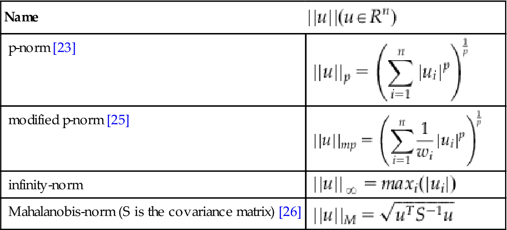
where ý is the measurement vector, á_i is the vector of the means of the RSSI values of each AP at the ith calibration point, and the norm ||·|| is arbitrary. Examples of possible norms are given in Table 1. The Euclidean norm (2-norm) is widely used, but the Manhattan norm (1-norm) is also common [23–25].

Table 1

Possible Norms

Name	$\left|\right|u\left|\right|(u\in R^n)$
p-norm [23]	$\left|\right|u|{|}_p={\left(\sum _{i=1}^n|u_i{|}^p\right)}^{\frac{1}{p}}$
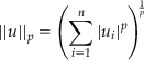modified p-norm [25]	$\left|\right|u|{|}_{mp}={\left(\sum _{i=1}^n\frac{1}{w_i}|u_i{|}^p\right)}^{\frac{1}{p}}$
infinity-norm	$\left|\right|u|{|}_{\infty }=ma{x}_i(\left|u_i\right|)$
Mahalanobis-norm (S is the covariance matrix) [26]	$\left|\right|u|{|}_M=\sqrt{u^T{S}^{-1}u}$

The estimator, that keeps the K biggest weights and sets the others to zero, is called the weighted K-nearest neighbor method (WKNN) [24]. The WKNN with equal weights is called the K-nearest neighbor method (KNN) [23]. The simplest method, where K=1, is called the nearest neighbor method (NN) [27]. In general, the KNN and the WKNN can perform better than the NN method, particularly with parameter values K=3 and K=4 [24]. However, if the density of the radio map is high, the NN method can perform as well as the more complicated methods.

4.2.1.2.2 Probabilistic Approaches

In the probabilistic (or statistical) approaches the state u is assumed to be a random vector [28]. The idea in the probabilistic framework is to compute the conditional probability distribution function $p_{u\vee y}(u|y)\triangleq p(u|y)$ (posterior) of the state u given measurements y. The posterior contains all the necessary information to compute an arbitrary estimation of the state. Using the Bayes rule we get

$p(u|y)=\frac{p(y|u)p(u)}{p(y)}$ (4)

(4)

where $p(y|u)$ is the likelihood, p(u) is the prior and p(y) is a normalizing constant. A conventional choice for the prior [28] is the uniform distribution, i.e.,

$p(u)=\frac{{\sum }_{i=1}^M{\psi }_{B_i}(u)}{{\sum }_{j=1}^M\left|B_j\right|}$ (5)

(5)

where |B_i| is the area of B_i and

${\psi }_{B_i}(u)=\{\begin{array}{c}1,u\in B_i\\ 0,u\notin B_i\end{array}$ (6)

(6)

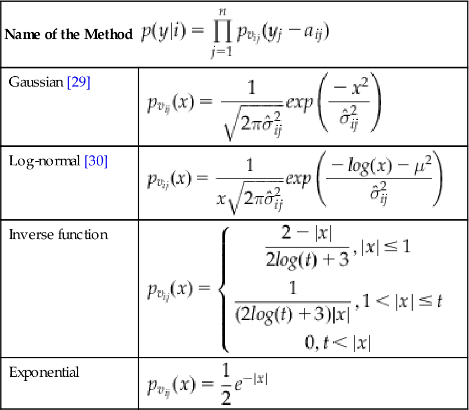
Assuming that the measurements collected at the calibration point represent the distribution of the RSSI in the whole cell (i.e., the likelihood is constant inside each cell B_i) the likelihood is

$p(y|u)=\sum _{i=1}^{M}p(y|i){\psi }_{B_i}(u)$ (7)

(7)

where $p(y|i)=p_{v_i}(y-a_i)$ and $v_i=y-a_i$. We assume that the components of the random vector v_i are independent. Thus,

$p(y|i)=\prod _{j=1}^n{p}_{v_{ij}}(y_j-a_{ij})$ (8)

(8)

where $y\in R^n$.

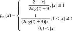
There are several approaches for computing the likelihood p(y|i). Examples of these methods are given in Table 2 [31].

Table 2

Likelihood Functions

Name of the Method	$p(y|i)=\prod _{j=1}^n{p}_{v_{ij}}(y_j-a_{ij})$
Gaussian [29]	$p_{v_{ij}}(x)=\frac{1}{\sqrt{2\pi {\hat{\sigma }}_{ij}^2}}exp\left(\frac{-x^2}{{\hat{\sigma }}_{ij}^2}\right)$
Log-normal [30]	$p_{v_{ij}}(x)=\frac{1}{x\sqrt{2\pi {\hat{\sigma }}_{ij}^2}}exp\left(\frac{-log(x)-{\mu }^2}{{\hat{\sigma }}_{ij}^2}\right)$
Inverse function	$p_{v_{ij}}(x)=\{\begin{array}{c}\frac{2-\left|x\right|}{2log(t)+3},\left|x\right|\le 1\\ \frac{1}{(2log(t)+3)\left|x\right|},1<\left|x\right|\le t\\ 0,t<\left|x\right|\end{array}$
Exponential	$p_{v_{ij}}(x)=\frac{1}{2}{e}^{-\left|x\right|}$

Substituting prior and likelihood equations into the posterior equation we get

$p(u|y)=\sum _{i=1}^M{\beta }_i\frac{{\psi }_{B_i}(u)}{\left|B_j\right|}$ (9)

(9)

From this posterior we can compute an estimate of the state u. One possible estimate is the maximum a posteriori (MAP) estimate. In this case, it is the same as the maximum-likelihood (ML) estimate, because the prior is uniform. The posterior is piecewise constant, and thus the MAP estimator is ambiguous. If the posterior has the maximum value only in one cell, say B_i, it is reasonable to use the center of the cell as the MAP estimate, i.e.,

${\hat{u}}_{MAP}=p_i$ (10)

(10)

Another commonly used estimate is the mean of the posterior, i.e.,

${\hat{u}}_{MEAN}=\sum _{i=1}^M{\beta }_i{p}_i$ (11)

(11)

Clearly, with fingerprinting there is a trade-off between the number of points in the grid (the larger this number, the more accurate the localization is) and the overhead due to the offline phase. In practice, the main drawback of this method is the high number of extensive and accurate measurements required during the offline phase to create the database. In fact, the creation of the database is not automatic: it is a human-based, time-consuming procedure and this is a practical barrier to wide adoption, because it makes the method unsuitable for rapid or ad hoc deployment. For these reasons, methods alternative to fingerprinting make use of signal propagation models, which are analytical models that relate RSS measures with distances [14,23,26,32].

4.2.2 Propagation Model

RSS is dependent on the environment, because the radio frequency signal suffers from reflection, diffraction, and multi-path effects that make the signal strength rather noisy. Consequently, localization systems based on signal propagation models need to calibrate parameters of the propagation model. The calibration procedure works in two phases: the training phase and the estimation phase. In the training phase, a set of RSS values are measured at a set of points in the area of interest; in the estimation phase, this information is used to estimate the propagation model parameters. The relationship between RSS and the reciprocal distance between anchors and mobile is then established by means of the calibrated propagation model.

Once a number of distance estimates between the mobile and the anchors are available, the most used algorithm to infer the mobile position is based on multi-lateration. As for the fingerprinting techniques, the localization based on the signal propagation model is expensive in terms of calibration time, since the calibration is not automatic. Moreover, the described calibration technique does not solve the time-dependent problem, since wireless channel variations affect the propagation model parameters, and this fact can significantly impact on the quality of the localization system. However, in recent works this problem has been solved by an automatic calibration procedure (called virtual calibration) of the signal propagation model that is only based on the RSSIs measured among the anchors and that can be executed periodically and automatically (i.e., without human intervention) [33].

4.2.2.1 Indoor Signal Propagation Model

Signal propagation is affected by many factors such as antenna height, antenna gain, antenna radiation pattern, transmitter-receiver distance, reflection, multi-path transmission, non-line-of-sight, obstructions, vegetation scattering and diffraction, RSS measurement uncertainty, etc. [34]. All these factors have to be considered when the distance estimation is calculated from the signal strength measurement. Several propagation models have been proposed [35]. They are characterized by different levels of complexity, depending on how many physical phenomena are considered. Basically, simpler models can be used when the environment characteristics are close to ideal conditions. Unfortunately, in most cases it is necessary to consider specific features of signal propagation in radio channels. In the literature most researchers model the indoor path loss with the one-slope model [36], which assumes a linear dependence between the path loss (dB) and the logarithm of the distance d between the transmitter and the receiver:

${L(d)|}_{dB}=l_0+10\alpha {\log }_{10}d$ (12)

(12)

where l₀ is the path loss at a reference distance of 1 m and α is the power decay index (also called path loss exponent). A generalization of the one-slope model is the two-slope model suggested in [37] to approximate the two-ray propagation model. Usually, in an urban environment, the two-slope model is characterized by a break point that separates the various properties of propagation in near and far regions relative to the transmitter: the path loss exponent changes when the distance d is greater than the break point. In particular, authors in [37] describe the existence of a transition region where the break point b is such that

$\frac{\pi h_t{h}_r}{\lambda }<b<\frac{4\pi h_t{h}_r}{\lambda }$ (13)

(13)

where h_t is the transmitter antenna height, h_r the receiver antenna height, and λ is the wavelength of the radio signal. However, in a typical sensor network scenario, the break point distance is on the order of hundreds of meters; therefore, in practice, the one-slope and the two-slope models are equivalent in indoor scenarios where the rooms are only a few square meters in size. Although the one-slope model is simple to use, it does not adequately account for the propagation characteristics in indoor environments. Indeed, one further generalization of the one-slope model consists of adding an attenuation term due to losses introduced by walls and floors penetrated by the direct path:

${L(d)|}_{dB}=l_0+10\alpha \mathrm{l}\mathrm{o}{\mathrm{g}}_{10}d+WAF{|}_{dB}+{FAF|}_{dB}$ (14)

(14)

where FAF|_db is the floor attenuation factor, and WAF|_db is the wall attenuation factor expressed as

${WAF|}_{dB}=\sum _{i=1}^N{K}_i{l}_i$ (15)

(15)

where k_i is the number of penetrated walls of type i, and l_i is the attenuation due to the wall of type i. Without loss in generality, assuming that sensors are all located on the same floor, the attenuation term due to the propagation among different floors can be neglected. A similar model was proposed in [38], where a multi-wall component is introduced, which includes the number of normal and fireproof doors and their status (open/closed) met by the direct paths. The received power RSS is obtained as the difference between the transmitted power P^t and L(d), i.e.,

${RSS=P^t-L(d)|}_{dB}=P^t-l_0-10\alpha {\log }_{10}d-\sum _{i=1}^N{K}_i{l}_i$ (16)

(16)

Letting $r_0=P^t-l_0$ be the RSSI at the reference distance of 1 m,

$RSS=r_0-10\alpha {\log }_{10}d-\sum _{i=1}^N{K}_i{l}_i$ (17)

(17)

This equation is used during the calibration procedure to estimate the propagation model parameters (r₀ , α, l_i ). In [33] the authors show that they are able to estimate the parameters of the chosen propagation model by exploiting the communications among anchors, without performing a preliminary measurement campaign.

4.2.2.2 Multi-Lateration Algorithm

In the last two decades, many localization techniques have been developed for wireless sensor network applications [39,40]. Among them, multi-lateration is seen to be one of the most popular localization techniques. Multi-lateration localization techniques form the basis of many other more sophisticated localization algorithms such as the iterative and the collaborative multi-lateration technique [39,41]. Multi-lateration is a simple localization technique that is based on distance measurements from multiple anchor nodes to the sensor node to be localized.

The sensor node location estimated by the multi-lateration localization technique is the one that minimizes the sum of squared distances between a hypothesized sensor location to all the anchor locations. Multi-lateration is a nonlinear optimization problem, although suboptimal linear optimization approaches can be applied. One of the major limitations of the classical multi-lateration localization approach is that it assumes that the anchor locations are error free and the only errors are in the distance measurements. This assumption is invalid in practice because the locations of anchor nodes are always inaccurate. There are, in general, two sources of errors for anchor location errors. The first source of error is due to the measurement errors of the anchor nodes. The second source of anchor location error arises when the locations of anchor nodes are only estimates. Some localization approaches such as AHLoS (ad-hoc localization system) [39] use an iterative process. For example, in AHLoS, some sensor nodes in the network first estimate their own positions based on broadcasted beacon positions. They then become anchors and broadcast their estimated positions to other nearby nodes for localization. The iterative process can lead to error propagation, resulting in large sensor location estimation errors as networks grow. The classical multi-lateration localization algorithms do not take into account and ignore the anchor location errors even though they exist. Recently, a number of approaches have been proposed to deal with the problem of anchor localization uncertainty for multi-lateration. In [42], the authors formulated the problem of multi-lateration in the presence of anchor position errors using the constrained least square technique (CTLS). The problem is then solved by using the Newton iterative algorithm. In [43], semi-definite programming (SDP) algorithms were proposed for sensor localization in the presence of anchor position uncertainties, and the corresponding Cramér-Rao lower bound (CRLB) was derived. In [44,45], a distributed localization algorithm was proposed based on second-order cone programming relaxation. In [46], an expectation-maximization (EM) estimator for localization of sensor nodes with erroneous anchor positions was proposed, which iteratively refines the anchor positions and estimates the sensor locations. A common disadvantage of the above mentioned approaches is that they all involve solving a nonlinear optimization problem.

Figure 4 shows the geometric relationship between the anchors and the node to be localized, where M anchors are used. In the figure, {x, y} are the unknown coordinates of the sensor node, {u_m, v_m} are the known coordinates of the m-th anchor and d_m is the estimated distance between the sensor node and the m-th anchor. Both the anchor locations and the distance measurements are assumed to contain errors. The multi-lateration localization approach is to estimate {x, y} given {u_m, v_m, d_m; m=1,2,…,M}. Denote

$g_m(\underset{¯}{x})=\sqrt{{(x-u_m)}^2+{(y-v_m)}^2}$ (18)

(18)

In general, multi-lateration minimizes the following sum of squared errors between the measured distances and hypothetical ones based on the unknown sensor node location [47]:

$\underset{x}{min}\sum _m{(g_m(\underset{¯}{x})-d_m)}^2$ (19)

(19)

Another technique [48] computes the intersection points among the three circles centered in a₁, a₂, and a₃; up to six intersection points can occur. Then, it estimates the position of the mobile {x, y} as the center of mass between these intersection points, i.e.,

$(x,y)=\left(\frac{{\sum }_{i=1}^n{X}_i}{n},\frac{{\sum }_{i=1}^n{Y}_i}{n}\right)$ (20)

(20)

In [29] context information provided by smart devices deployed in the environment is exploited by the localization algorithm in order to improve the performance in terms of localization error. In [49] the authors propose a decision tree algorithm to select the candidate intersection points that better provide the location of the mobile.

4.2.2.3 Maximum-Likelihood Distance Estimator and Cramér-Rao Bounds

The Cramér-Rao bound can be used to compute the theoretical attainable performance of localization systems that exploit RSS measurements. In this section, we derive the expression for the maximum-likelihood estimators (MLEs) and the Cramér-Rao bound (CRB) for the estimation of the distance between the mobile and the anchors. The properties of the bound on localization error may help in designing efficient localization algorithms; moreover, it provides suggestions for a positioning system design by revealing error trends associated with the system deployment. We derive the expressions for both the case of a single RSS value and for the more interesting cases of multiple RSS values used to estimate the distance.

4.2.2.3.1 RSS Information: Single Sample Case

The mobile device periodically receives the beacon signal sent by a given anchor and registers its RSS value r, which can be modeled as a Gaussian random variable. Thus, we have

$rN(R,o^2)$ (21)

(21)

and, from the relationship between RSS distance already explained in section 4.2.2.1, i.e., $RSS=r_0-10\alpha {\log }_{10}d-\sum _{i=1}^N{K}_i{l}_i$, the probability density function of r conditioned on the distance d between the mobile and the anchor is

$f_d(r)\propto \frac{1}{d}\exp \left[\frac{{(r-R)}^2}{-2o^2}\right]$ (22)

(22)

Then, the maximum-likelihood estimator of d is

$\hat{d}=arg\underset{d}{max}{f}_d(r)$ (23)

(23)

In order to evaluate such maximum, we differentiate the log-likelihood function, obtaining the following function:

$\frac{\partial }{\partial d}ln{f}_d(r)=A\sum _{i=1}^N\frac{(r-R)}{o^{2}d},\mathrm{being}A=10\alpha lo{g}_{10}e$ (24)

(24)

therefore

$\frac{\partial }{\partial d}ln{f}_d(r)=0\Rightarrow r-R=0$ (25)

(25)

and thus

$\hat{d}={10}^{(r_0-r-L_w)/10\alpha }$ (26)

(26)

The Fisher information I measures the amount of information that a random variable carries about an unknown parameter. Here the random variable is r, and d is the unknown parameter. The inverse of the Fisher information, known as the Cramér-Rao bound, is the minimum variance that can be achieved when estimating d by using any unbiased estimator. By evaluating the Fisher information for RSS measurements (details to compute the Fisher information are presented in [36]) we can identify the minimum theoretical error for the distance estimation. The Fisher information associated with RSS measurements is

$I_d=E_d\left[{\left(\frac{\partial }{\partial d}ln{f}_d(r)\right)}^2\right]=\frac{A^2}{{\sigma }^2{d}^2}{E}_d\left[{(r-R)}^2\right]={\left(\frac{A}{\sigma d}\right)}^2$ (27)

(27)

hence, the CRB entails

$\sqrt{\mathrm{Var}(\hat{d})}\ge \frac{\sigma d}{A}$ (28)

(28)

4.2.2.3.2 RSS Information: Multiple Samples Case

In order to improve localization accuracy, multiple RSS samples are normally used to estimate the distance between anchors and mobile; as already stated, we assume that the RSS values r are i.i.d. random variables. We assume that the mobile device did not move significantly in the measurement time span during which the RSS samples are collected. Being (r₁, … , r_N) independent random variables, the joint PDF conditioned on the distance d is

$f_d(r_1,\dots ,r_N)\propto \prod _{i=1}^N\frac{1}{d}\exp \left[\frac{{(r_i-R)}^2}{-2o^2}\right]$ (29)

(29)

Following the same steps as in the previous case, we obtain

$\frac{\partial }{\partial d}{\mathrm{lnf}}_d(r_1,\dots ,r_N)=A\sum _{i=1}^N\frac{(r_i-R)}{o^{2}d}$ (30)

(30)

therefore

$\frac{\partial }{\partial d}{\mathrm{lnf}}_d(r_1,\dots ,r_N)=0\Rightarrow \sum _{i=1}^N{r}_i-R=0\Rightarrow \frac{{\sum }_{i=1}^N{r}_i}{N}=R$ (31)

(31)

and thus the MLE of the distance is

$\hat{d}={10}^{(r_0-r_i-L_w)/10\alpha }$ (32)

(32)

The Fischer information is

$I_d=E_d\left[{\left(\frac{\partial }{\partial d}{\mathrm{lnf}}_d(r_1,\dots ,r_N)\right)}^2\right]=\frac{A^2}{o^2{d}^2}{E}_d\left[\sum _{i=1}^N{(r_i-R)}^2\right]={\left(\frac{A}{od}\right)}^{2}N{o}^2={\left(\frac{A}{od}\right)}^{2}N$ (33)

(33)

hence, the CRB is

$\sqrt{\mathrm{Var}(\hat{d})}\ge \frac{od}{A\sqrt{N}}$ (34)

(34)

5 Conclusions

The world of personal localization using wearable devices or no devices at all is rapidly evolving, yet no single solution has yet emerged as the killer application. Working commercial or prototyping solutions that are general enough to be of practical usage in indoor environments are based on RSS measurements of packet radio signals, ultrasound, and MEMS (micro electro-mechanical systems) such as those found in smartphones. A fusion of inputs from more than one technology is commonly used, but the most powerful fusion systems cannot run on the wearable devices: rather, they run on external servers that are part of the local infrastructure.

Exceptions to this rule are starting to appear: PDR (pedestrian dead reckoning) systems have reached a level of maturity that allows them to run on a smartphone at a level of accuracy sufficient for navigating a building even without assistance from the environment, but with the option to fuse information obtained from the local infrastructure.

Any recommendation pointing to a specific technology would be obsolete the moment it is written, as low-price commercial offerings are starting to come out and academic research is fast progressing. As an example, let’s examine the criteria to consider for evaluating a smartphone-based PDR system. Since these systems are resource intensive, it is important to verify the requirements imposed by the application on the smartphone, in terms of CPU power, sensor availability, and most importantly, battery consumption. Systems that do not require a preliminary training phase should be preferred; preference can turn into a requirement if the application is going to be used occasionally, for example, for visitors. It should be possible to have the choice of downloading a complete map of the environment, for offline use, or getting partial maps on demand, in order to speed up starting times and minimize memory and network usage. Some systems are able to track the position even without a map: this can be useful to get back on one’s step, or to superimpose the recorded path once the user obtains a map of the environment, or even to create a map of the unknown environment. The more sources of information the system manages to fuse together, the better: for example, an application could be able to run on a low-range smartphone without a compass or a pressure sensor by exploiting a map of wifi access points in the environment, at the price of lower accuracy and higher battery consumption.

In the future we foresee several methods being used on different devices, and different sources of information being exploited depending on the computing capabilities of the portable or wearable devices. More specifically, we see two trends. The first, consequent to the diffusion of ever more powerful smartphones, will push toward the use of PDR methods fused with compass and atmospheric pressure information for smartphones. The second, because of ubiquity of devices communicating through packet radio in smart environments, will push toward RSS-based methods to be implemented in small devices collaborating with local infrastructure. The two trends will merge and coexist in flexible ways, depending on the capabilities of the wearable devices and on the services offered by the local infrastructure.