If your project has required deeper Six Sigma statistical analysis, you’ve been waiting for this time ever since you started your project. Everybody on your team, the Process Owner and all the stakeholders, have ideas about how to fix the process and solve the problem. Each of your team members has probably kept a list, or parking lot, of solutions in his or her head or on paper. Some of these ideas were disproved through data collection and analysis, while others were reinforced.

Now is the time to generate several possible solutions to your problem, along with their corresponding action plans. That’s why this chapter will show you how to refine your Y = f(x) pathway, driving all the way to the point where you know the ultimate answer to your performance problem! If you know the answer, you can develop different solution alternatives, ultimately choosing the best for full-scale implementation.

As you review and consolidate your analysis work, solutions will fall into three categories: 1) the solution will be obvious, so just do it! 2) the team knows where to focus but needs to refine the solution(s) and corresponding Implementation Plan; 3) you need a miracle or an innovation to solve the problem.

Regardless of your pathway, you want to find solutions that are long-lasting and permanently address the root cause of your problem. You either want to eliminate that root cause or change the process to function as desired regardless of that cause (robust design). In any case, you’ll want to update your Critical X Worksheet (from Chapter 16) to reflect what you’ve learned and confirmed since the Analyze phase.

Your goal is to generate a complete list of possible ways to solve the problems at hand, using the investigations and factual data you’ve collected. Your list of potential solutions is probably not complete, and your team needs to expand its solution ideas before rushing into the first one it has. Brainstorming and inventive problem-solving techniques can provide unique solution ideas.

By solving your primary problem, it’s likely that you’ll surface other, lower-order problems that need to be solved. In addition to solving your primary problem, your proposed solutions will also have to address these related but subordinate problems. Hint: If the subproblems are extremely difficult or complex, they might require a separate or parallel DMAIC effort. If not, you can usually address them using simple brainstorming.

Start by identifying these lower-order problems and ask “How to …” in front of each one. This will focus the brain on coming up with necessary solution actions, which later can become the line items of your Implementation Plan.

For example:

Brainstorming techniques open up the creativity side of your brain, bringing out unique perspectives for solving problems. Most brainstorming techniques are divergent in nature, meaning they expand your list of possibilities according to some spawning mechanism. Some of these methods include …

To achieve a breakthrough in your solutions, sometimes an innovation or invention is needed. While the multitude of brainstorming techniques tend to be focused on expanding your thought horizon, a handful of techniques are available that rely on inventive benchmarking for similar problems. Such benchmarking is convergent rather than divergent in nature—you work your way to a specific solution through the use of established inventive principles and the use of thinking by analogy.

The Theory of Inventive Problem Solving (a.k.a. TRIZ) was developed by Genrich Altshuller after studying the principles behind thousands of patents worldwide. TRIZ focuses on specific problems, leading the practitioner to a proven matrix of generic solutions, which then are translated into specific solutions via analogical thought.

To generate potential solutions, TRIZ starts with the Ideal Final Result (IFR)—a perfect solution with no trade-offs or negative consequences. TRIZ measures the deviation (trade-offs) of proposed solutions from the IFR; these potential trade-offs then become contradictions for TRIZ to solve.

Once the contradictions have been formed into a problem statement, they are re-phrased as conflicts between generic parameters, of which there are 39 in the TRIZ system. The TRIZ practitioner then references the parameters in a contradiction matrix to reveal the inventive principles by which others have solved similar problems (contradictions) in other environments at other times.

Using these principles, the innovator can then analogously reason his or her way back to a specific solution to a specific problem. That, in a nutshell, is a convergent approach for coming up with viable inventive ideas for solving problems. TRIZ and other structured innovation approaches are a burgeoning field as extensive and deep as Lean Six Sigma.

You can also use Lean concepts and techniques to come up with potential problem solutions, especially when trying to improve Flow and Pull for the purpose of reducing waste and increasing efficiency. We covered the most widely used techniques in Chapter 17, so check out that chapter for more details.

In Chapter 17, we talked about creating a future-state Value Stream Map as a framework within which to guide solution generation. Here we revisit this theme with the following guidelines, in case you need more help using process thinking to generate potential problem solutions.

So you’ve got a bagful of solutions now, or at least a couple of solid options. Of course, all your solution-generation activities have been constrained by your discovery during Analyze and Improve. So all possible solution options should be solid, and you should have a high degree of confidence that they will solve your problem and improve performance.

Still, not all solutions can be put into action plans immediately. You have to evaluate the viability of implementing each of your proposed solutions in the spirit of managing limited resources, avoiding unnecessary risk, and accomplishing your gains in a realistic time frame.

Once a number of alternative solutions have been identified, similarities between solutions can be identified through Affinity Diagrams. If you’re not familiar with this tool (Affinity Diagram), see Chapters 13 and 22 for some details. Basically, Affinity Diagrams enable you to organize your brainstormed solutions into proposed Action or Implementation Plans.

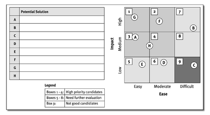
Another way to narrow down your solution options is to subject them to two simple criteria: their quality (Impact) and their efficiency of implementation (Ease). Just plug your potential solutions into the following Ease/Impact Matrix to see where they fall in the resulting nine-box grid.

The Ease/Impact grid compares the impact of each potential solution and the ease of getting the solution in place. Relative positions on the grid help determine the priority of each solution.

The Impact of a solution is estimated by projecting its benefits according to project metrics, and its longevity. Of course, the acid test for Impact is to evaluate the solution 12 months after its full implementation. But right now that’s getting the cart a little before the horse.

Ease is focused on the politics, technology required, difficulty of implementation, and time frame required for implementation. Just Do It solutions rate on the easy end of the spectrum. Solutions with political, technical, or cultural barriers rate as difficult. Solutions requiring high capital investment or long lead times also rate as difficult.

So here’s the skinny. Solutions in boxes 1 through 4 are high-priority candidates. Solutions in box 5 might get some quick wins, but have little impact on your metrics. Solutions in box 6 should be further evaluated to see if they can be combined with other solutions to achieve a stronger impact. Solutions in boxes 7 and 8 might need intervention by a Champion to improve the ease of implementation. Finally, solutions in box 9 are not good candidates for adoption.

Experimental trials in the Analyze phase were primarily focused on screening out insignificant xs and finding the critical xs. Now that you have more direction with the potential solutions, you’ll probably need to refine your knowledge of the critical xs before proceeding with pilot trials and a specific solution Implementation Plan.

We introduced Monte Carlo and discrete simulations in the Analyze phase (Chapter 16). The first step was to model the As-Is process and identify bottlenecks and sensitivity to critical xs. Using simulations, you can manipulate the critical xs to see how they impact the overall process. If one process step has large variation, the simulation can examine the impact of reducing that variability or adding additional resources.

If the results of the simulation are positive, you can seek solutions to reduce the variability of the process step. Of course, the solutions will still require validation prior to pilot trials of the revised process. For more complex analysis, simulations can be combined with DOE methods to identify the solutions with the greatest impact.

Well-designed experiments extract concrete evidence of the x-Y relationships and provide clean data for defining Y = f(x). Once again, DOE is the answer. Specifically, you can use Response Surface Methods to examine for responses that have curvature and/or interaction effects.

Let’s look at an example of trying to adjust the friction index of a brake lining. The goal is to center the friction index on a target of 25 with minimal variation. Three critical xs were identified in the Analyze Phase: Temperature, Time, and Pressure.

A Box-Behnken Design is chosen for the response surface design setup. This design incorporates three levels of each factor and three center points—a total of 15 combinations.

The use of the Box-Behnken Design provides clean data, free of correlation between input factors, while providing the necessary trial combinations to establish higher-order quadratic and interaction terms in the equation.

Once a prediction equation is developed, optimization methods or Monte Carlo simulations can direct the team to optimal conditions for the process. For our friction index example, three samples were tested for each trial (F1, F2, and F3). The mean and standard deviation for friction index were analyzed using Regression Analysis.

The regression model is reduced to the significant terms and a prediction equation is written in uncoded terms (i.e., actual units) for temperature and time.

Performing regression analysis on the standard deviation for each trial showed that temperature and time were significant terms. Interaction and quadratic terms were not statistically significant and not included in the equation.

The contour plot for the average friction index, following, shows curvature from the quadratic Temperature term. The contour line at 25 shows the multiple combinations of Temperature and Time that can be used to set the process mean on target. The contour plot for standard deviation shows a linear relationship, with lower variability in the upper right-hand corner of the plot.

Contour plots can graph equations for varying levels of two factors, with the response variable shown in the contour regions.

By overlaying contour plots, the region of most interest is highlighted—on target with low standard deviation. This technique is handy with two dominant factors, but more complicated with multiple critical factors.

Optimization routines use linear algebra or more complex search methods to determine the best settings of factor levels to meet performance criteria. Comprehensive statistical software packages can seamlessly optimize the settings after analysis of designed experiments. Upwards of 20 Y responses can be optimized with upwards of 20 input factors with relative ease.

Verification trials should always be run to confirm the output of the optimizer before proceeding to pilot trials.

Monte Carlo Simulation uses fundamental models incorporating variability in factors to generate results based on the Y = f(x) equations. Input factor levels can be varied with realistic distributions, decision rules, and constraints to simulate the real process. Many simulation packages also include search methods to pinpoint optimal conditions based on the models.

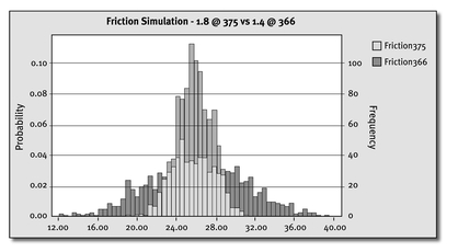
This output from Crystal Ball^® software compares two feasible solutions to meet the average friction index. Input Temperatures and Times were varied through specified input distributions to simulate process operating conditions.

DOE can also be used to evaluate multiple solutions to a problem on a small scale prior to piloting the solutions. If multiple individuals are working in the process, DOE combinations can be divided amongst them to match the design combinations.

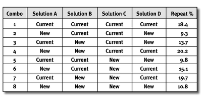
As shown by the following table, each solution is placed in the design matrix as a factor, with the levels set at either adopting (New) or not adopting (Current) the solution. The advantage of the DOE, versus trying one factor at a time, is that each solution has been tried multiple times in combination with other solutions.

Four proposed solutions were compared in eight combinations via a designed experiment. The levels for each solution were to stay with the current or implement the new solution.

Example: A project team was working to reduce the number of repeat calls from 18 to 8 percent at its customer service centers. In the Improve phase, the team identified four independent solutions that would require varying levels of training and resources to implement.

A designed experiment was created to evaluate the potential solutions in eight total trials. Customer service representatives at one of the centers were divided into eight groups and the eight combinations of solutions were tried for three weeks.

The results showed that one solution reduced repeat calls by 7 percent, while another increased repeat calls by 3 percent. The other two solutions had smaller, but positive impacts on reducing repeat calls. Two of the solutions were implemented and the goal was reached.

The Least You Need to Know