Chapter 16
Solve the Problem
In This Chapter
♦ Getting your priorities in order
♦ Torturing the xs to get a confession
♦ Experiment like you never have before
♦ Simulate processes to gain profound knowledge
♦ On the road to Y = f(x)
Reviewing log sheets, analyzing computer databases, detailing failure modes, and conducting special studies should be giving you a clue about the xs that have the most impact on Y. So far you’ve collected data and analyzed, but you really haven’t changed much. The latter part of the Analyze phase and the Improve phase focus on manipulating the xs and detailing the results.
In this chapter, we crank it up a notch. We’ll bring in the most likely x suspects and torture them until they finally confess. Which ones are significant? Which have the leverage? This is our focus in this chapter. To accomplish this, we’ll cover such key Lean Six Sigma tools and techniques as correlation, Design of Experiments, Analysis of Variance, and simulation.
Prioritize the xs
Early in Analyze, you identified potential xs using a Cause-and-Effect Matrix, mostly with opinions from your team. You also examined failure modes using FMEA techniques and established Risk Priority Numbers (RPN) based on the Severity, Occurrence, and Detection of process failures. Your review of the process through Lean glasses identified waste, Flow, and efficiency issues. Now it’s time to bring that analysis together and track down the really important xs.
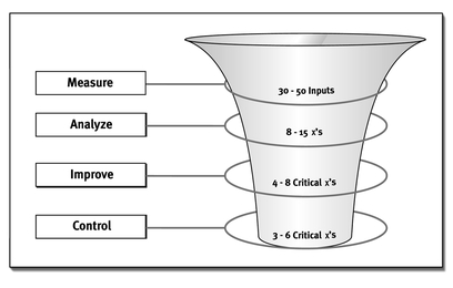
Initial Cause-and-Effect Analysis in the Measure phase should identify a vast number of potentialxs. The Analyze and Improve phases narrow the list down to the vital few that make the most significant impact.

Real-Life Story
A team focused on improving the flatness of the disk in a hard disk drive—a key component of performance. The intial fishbone identified 30 potential xs that might affect flatness. Through a series of designed experiments, the team investigated each x and found that number 17 had the biggest impact on flatness, and a breakthrough was achieved!
Focus on the Primary Metric
The success of your project relies on the team’s ability to improve the primary metric (Y). Your initial opinions on the fishbone diagram directed your data collection. The data became information through process, graphical, and statistical analyses. You now need to turn that information about the process into knowledge. The next step will be to turn the knowledge into action—the Improve phase of DMAIC.
The Critical X Worksheet is a log of your analysis to date, sorting out the significant xs from those that don’t have leverage to impact your process. As you can see from the following sample, the Critical X Worksheet summarizes the impact of each x on Y, and shows the evidence supporting that claim.
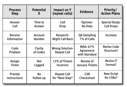
This Critical X Worksheet sample shows five critical xs that were surfaced as a result of analysis.
Revisit the Cause-and-Effect Matrix
The Cause-and-Effect Matrix shows the impact of each x on all the Ys. Early in Analyze, you developed a C&E Matrix with the team, with the best knowledge at hand. Now that your knowledge is more refined, you need to update the C&E Matrix. The C&E Matrix is an evergreen document—it should be updated whenever the knowledge of the x-Y relationships is improved.
Evaluate the Impact on Y
Databases, log sheets, and observations can surface the high-level suspect xs from the crowd, but you need more than that. You need to verify the impact of those xs on your primary metric. Statistical analysis of historical data can yield correlation of x variables with Y, but often the x variables are also correlated with each other, leaving doubts about which x might cause Y to vary.
The correlation coefficient (r) is used to quantify the linear relationship of the variables. The correlation coefficient varies between -1 and +1, with 0 representing no correlation. If the variables are plotted on a Scatter Plot and all the points fall perfectly on a straight line, the correlation coefficient will be -1 if the slope is negative, or +1 if the slope is positive.

Lean Six Sigma Lingo
Correlation is the strength of the relationship between two variables. Correlation can be used to identify x-Y relationships, or x-x or Y-Y relationships. A high correlation does not necessarily imply that one variable causes the effect of the other variable.
Wayne and Fred collected detailed data for a day of fishing. They correlated two Ys (Fish Weight and Time to Catch) to five xs (Time of Day, Depth, Bait, Location, and Sky). Fish Weight had a high correlation with each of the xs, but the xs were also highly correlated with each other. Which x really caused the Y to change? Even sophisticated regression analysis can’t sort this one out.
This Matrix Plot shows the various correlations between Wayne and Fred’s fivexs and two Ys. It also shows the correlations of all five xs with each other.

Since correlation coefficients examine one x at a time versus Y, you need to watch out for four possible pitfalls that can occur in the analysis:
♦ Variation in other xs can mask the correlation of the x under examination.
♦ Correlation of input xs can lead to mistaking the effect of one x for the true effect of the critical x.
♦ Two xs might combine to produce a significant interaction effect in Y that is not apparent for either x when examined individually.
♦ Nonlinear effects do not show up as strong linear correlations.
Correlation studies are most useful when only one or two xs create most of the variability in Y. When multiple xs are under investigation, you need more sophisticated methods like Design of Experiments (DOE), Analysis of Variance (or ANOVA), or simulation methods. We’ll look at each of these now.

Real-Life Story
An analyst was trying to correlate the impact of several operations on the end result—late mail. Substantial information on 16 metrics had been collected and each was tested individually for correlation. None were significant. When the analyst used multiple regression analysis that included all the xs, significant effects were found. The multiple regression partitioned the effect of each x so that it would not mask the effect of other xs.
Design of Experiments
At some point, you’ll need to experiment with xs in the process—and you need to do so in the most reliable and cost-effective way possible, with experiments that yield easy-to-understand conclusions. DOE methods do just that—if you can properly manipulate your xs for special study.
Design of Experiments uses specific design combinations (arrays) of changes (levels) of input factors (independent variables) to observe changes in output responses (dependent variables). A key characteristic of DOE is to eliminate any correlation of input factors and to extract the contribution of each factor.
DOE can be used to stratify the effects of each input factor independently of the other factors. This is accomplished by the use of orthogonal arrays that are analyzed for the effects of each factor, and any interactive effects. The simplest design would be a two-factor design, with each factor varied over two levels.
To demonstrate a simple DOE, here is an actual example. One of the authors of this book was driving from Pittsburgh to Denver in his van and thought a DOE on gas mileage would be entertaining. He selected two inputs he could control—Gas Octane at two levels (86 versus 91) and Speed at two levels (55 mph versus 65 mph). All combinations of the factor levels would require four trials, as shown by the following figure.

Lean Six Sigma Wisdom
Design of Experiments techniques were first used in the 1920s to improve crop yields in England by Sir Ronald Fisher. Since that time, the methods have been used by American universities and by many industries around the world to develop and improve products and processes.

The design array for a two-level design is typically written as “-” for the low level of a factor and “+” for the high level. The four combinations shown are translated into the actual experimental conditions. Other columns can be calculated to represent interaction effects (X1X2) but are not needed to set up the experiment.
For this experiment, gas mileage varied from 21.0 mpg to 24.2 mpg—more than expected. To analyze the results, we calculate the difference in averages for each factor level.
The average with 91 octane is 22.6 mpg, and the average for 86 octane is 22.5 mpg. The difference of 0.1 mpg seems rather small. For speed, the average at 65 mph is 21.1 mpg and the average at 55 mph is 24.0 mpg—a difference of -2.9 mpg!
The effect of the interaction can also be calculated using the “+” and “-” levels of the interaction (see the following diagram). The “+” level averaged 22.4 mpg and the “-” level averaged 22.7 mpg—a difference of -0.3 mpg—negligible compared to the speed impact alone.
The Main Effects Plot shows the averages for each factor level. The Interaction Plot shows the combination effects of two factors.
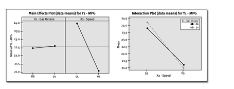
By viewing the Main Effects Plot, we can conclude that speed affects gas mileage significantly, and that the octane level does not affect gas mileage significantly. We can also conclude that the combination of speed and octane level produced no significant interaction effect. (Parallel lines on an Interaction Plot indicate no interaction effect.)
Maybe we can provide you a few helpful hints about how to make your DOE as smooth, efficient, and errorless as possible. Here’s some simple advice:
♦ Don’t put all your data eggs in one basket. Projects have relied on downloading computer databases only to find that many of the xs were not in the database.
♦ Make sure measurement systems are accurate and precise. Poor measurement and recording of xs causes biases and lack of precision in the data, leading to analysis errors.
♦ Drill down to find the critical xs. Teams that don’t stratify the layers of xs gloss over significant differences and abandon the hunt for the critical xs.
♦ Go beyond the typical variation in xs if necessary to see the x-Y relationships more clearly. If the xs vary little in your data, you may need to manipulate them to uncover the relationships.
♦ Take sufficient samples before running statistical tests. Not collecting enough data is coming to court with no evidence—the guilty x is likely to go free!
♦ Involve stakeholders in the data collection plan. People in the process can identify flaws in the plan and identify other significant xs.
Analysis of Variance
Analysis of Variance (ANOVA) is the statistical method used to test the hypothesis that changes in levels for each x factor cause changes in the response variable Y. ANOVA partitions the explained variation in the response variable for each factor or interaction, and also creates an error category for unexplained variation.
For each factor, the explained variation is weighed against the unexplained variation to determine if the results are statistically significant for the amount of data collected. A p-Value is calculated for each factor to determine the risk of making a Type I error (calling a factor significant when it is not). Generally speaking, a factor is considered significant if its p-Value is less than 0.05.
Many factors can be investigated at many levels in designed experiments. Experiments that test all combinations of factors and levels are called full-factorial designs. Fractional factorial designs are also available to significantly reduce the number of trials, while retaining the integrity of a statistically designed experiment.
Simulation
While DOE methods, including ANOVA, provide solid evidence for identifying the critical xs, the resources required might be prohibitive. (Running such statistical tests can be expensive and time-consuming.) Another alternative for process analysis is the use of simulation techniques, such as Monte Carlo Simulation, when the parameters and relationships of the xs are known, but the overall system is complex.

Lean Six Sigma Lingo
Monte Carlo Simulation uses mathematical models, probability, decision rules, and induced variabililty in inputs to simulate real-life scenarios and identify variability in outputs.
The advantage of simulation compared to deterministic spreadsheet models is that a range of inputs are investigated, and the range of outputs are quantified, versus a single output from a deterministic model. Therefore, the sensitivity of the outputs to variation in inputs can be identified and prioritized. For example, let’s examine a loan approval process to determine where the overall cycle time can be improved.
This six-step process takes 100 hours on average, according to the average of individual process steps. Simulation of the process using Monte Carlo methods includes the rework in the process, variability, and distribution of process times.
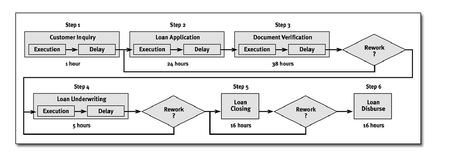
This output from Crystal Ball® software shows the variability of loan cycle times based on variability and defect levels for the six process steps. We added the sensitivity analysis to show that the total cycle time is predominantly dependent on delays in document verification.

Monte Carlo Simulation is not limited to process analysis. It can also be used for tolerance design of parts, probabilistic models (e.g., on-time air travel), and a variety of other investigations. To develop a good simulation model, the team must first detail the as-is process prior to playing what-if scenarios or redesigning the process.
Switching gears, Discrete Process Simulation models show the visual flow of materials through the process to help identify bottlenecks and utilization of resources. The model is based on a process flow model, with the ability to incorporate decision rules, queues, assignment of resources, and work schedules. An example of Discrete Process Simulation follows.

A Priority Mail team used the process flow diagram and ProcessModel software to conduct Discrete Process Simulation analysis of a new facility.
Prior to building facilities to process Priority Mail, an improvement team used Discrete Process Simulation models to determine the flow of mail, and to identify bottlenecks in the proposed process. Inputs were based on the operations in current facilities and experimental trials for process changes.
Resources were assigned by the software for each process step, and task time distributions and volume fluctuations were included in the model. Bottlenecks and the impact of defective units were identified through the simulation.
The model showed that mail arriving on the last truck of the night needed to be processed through a different flow to meet the outbound schedules. It also showed that a large bottleneck would occur at final dispatch late in the shift. The process was redesigned, which led to the avoidance of the bottleneck at the opening of a new facility.
State the Y = f(x) Equation
The Y = f(x) equation represents the dependence of the output response on the input factors. The output might be a probability of occurrence or a continuous response.
The input factors might be continuous or discrete (categorical). Some of the input factors identified will be controllable, others might be noise (e.g., temperature, or arrival rates of customers).
For many projects, a specific mathematical Y = f(x) equation can be stated. Other projects may find the impact of critical xs is well understood, but trying to put them all into a single mathematical equation just doesn’t work. In these cases, knowledge of the impact of each x can still be used to improve and optimize the process.
Designed experiments produce results that can easily be transformed into Y = f(x) equations. If the xs are continuous, the equation can be written as a true mathematical equation. If the xs are discrete, the equation looks a little different—the effect of each depends on which categorical level is chosen.
Good analysis of data, experimental trials, and simulations can weed through the previously unexplained variation and explain why the variation occurs. Regression analysis and ANOVA separate the total variation into two components—factor effects (explained) and error (unexplained variation).
A company that manufactured water meters discovered that the see-through lids were cracking when the screws were tightened down. The team developed a torque test to investigate the settings and material on the plastic injection molding machine that produced the lids. Having identified 11 potential xs on the molding machine alone, the team conducted a screening DOE consisting of 12 trials. The results from the experiment identified three critical xs, leading the team to produce lids that didn’t crack on assembly.
This was a 12-run Placket-Burman screening design. Eleven factors (X1—X11) were run at two levels each. Instead of running all 2,048 combinations, the highly fractionated factorial design only required 12 experimental combinations.
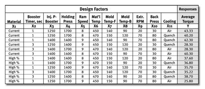
DOE uses ANOVA to separate the statistically significant xs from other unproven xs. For our injection molding example, 12 data points were recorded, allowing for 11 terms in an equation plus a constant. Variation is stratified for each of the 11 factors by using a Sum of Squares accounting method.

The differences in average torque were calculated by comparing the means of the + level to the - level of each factor. Three factors show more than a 3-torque unit’s effect on the average torque values: Booster Seconds, Ram Speed, and Mold Temp-Back.
The following ANOVA table is then constructed by separating out the major contributors to variability (explained variation) and pooling the variation from minor contributors into error (unexplained variation). The explained variation is compared to the unexplained variation using an F-test and results in a p-Value for each factor. The p-Value represents the alpha risk of calling the factor significant when it is not. Confidence in your decision is defined as (1-p).

Technically Speaking
The F-test is used to determine if variances are different comparing variability between means of multiple populations (variance between groups) to the variability within the populations (variance within groups).
It’s really great to have a Y = f(x) equation finally, but do we really have the whole picture? Using a table of level effects, which follows, predictions can be made about the torque values for any of the 2,048 possible combinations, even though only 12 experimental combinations were run.
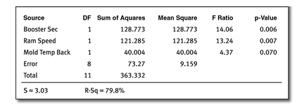
For the injection molding example, the ANOVA table was reduced from 11 factors to 3 major contributors, and 8 terms were placed in error. The result was an R-squared value, showing that 79.8 percent of the variation in the experiment was explained by the three major terms. The 20.2 percent unexplained variation is assumed to be random error and contributes an estimated standard deviation of 3.03.
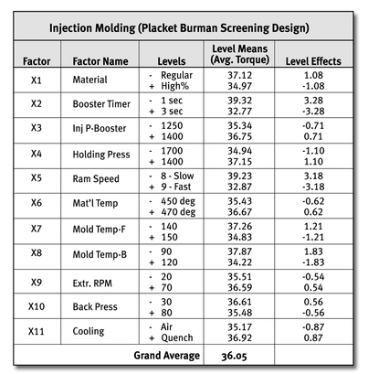
A table of level effects shows the mathematical effect of changing levels for each factor tested. A conservative approach to making predictions would be only including factors found to be statistically significant.
To predict the best combination of settings from our example, we would select the levels of the three significant factors that increase torque values:
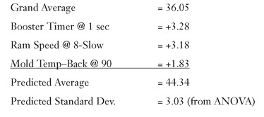
Based on the analysis, you can also make predictions for other combinations, and you can run verification trials to confirm the predictions. At the end of the rainbow, you still might not be able to state the exact Y = f(x) equation—but that’s your goal, and you shouldn’t stop your analysis until you can do this.
Conduct Tollgate Review
Before moving on to the Improve phase in the next chapter, you need to conduct a tollgate review that ensures you’ve accomplished all your critical tasks. This review should be attended by your Lean Six Sigma Champion, your Process Owner, team members, and other key stakeholders. Some questions to ask, and answer, at your review include:
♦ Has your problem or objective statement changed? (Answer: If not, great. If so, reflect changes on your Project Charter.)
♦ How did you identify potential xs? (Answer: Show correct use of Process Map, Brainstorming, Affinity Diagrams, Fishbone Diagrams, etc.)
♦ What xs were verified with data? What evidence do you have? (Answer: Used Scatter Plots, Hypothesis Testing, ANOVA, Regression, etc.)
♦ What are the top potential process steps, based on RPNs, that you have identified from your FMEA? (Answer: see completed FMEA.)
♦ What has the performance been, by week, for the metrics tracking your primary metric? (Answer: We maintained a Control Chart or Time Series Plot.)
♦ If you have completed the Analyze phase, what are your conclusions? (Answer: We know what our critical xs are with a specified degree of confidence.)
♦ Was a preliminary Y = f(x) equation developed (to be refined in the Improve Phase)? (Answer: Yes, and here is the proof.)
♦ Have you developed a plan for and conducted Design of Experiments? (Answer: We did, and here is our data and conclusions.)
♦ Are all data fields in your project tracking tool current with your most recent project progress? (Answer: Hopefully yes. If not, enter data.)
♦ Are you satisfied with the level of cooperation and support you are getting to solve your project in a timely manner? (Answer: If yes, great; if no, revisit Stakeholder Analysis and Action Plan.)
♦ Is your project still on track to meet the scheduled completion date? (Answer: If yes, great; if no, remove roadblocks, accelerate pace, lead, revisit Stakeholder Analysis.)
♦ Has your financial forecast changed by more than 20 percent? If yes, what is the new validated forecast? (Answer: With the finance rep, we updated the project forecast.)
The Least You Need to Know
♦ You cannot investigate all the xs—you need to prioritize your investigations to the most likely.
♦ Continue to update the Cause-and-Effect Matrix and FMEA to document your knowledge of the process.
♦ Pitfalls in correlation analysis can be prevented by using Design of Experiments methods and ANOVA analysis.
♦ Simulation techniques can provide insights to the critical xs when physical trials are prohibitive.
♦ Advanced statistical tools such as regression analysis, DOE, and simulation can develop Y = f(x) equations. Verification of the predictions is mandatory.
..................Content has been hidden....................
You can't read the all page of ebook, please click here login for view all page.
