
CHAPTER 17
ELECTRIC PROPULSION
Chapters 1 and 2 present information on rocket propulsion devices that use electrical energy for heating and/or directly ejecting propellant thus utilizing an energy source that is separate from the propellant itself. The purpose of this chapter is to provide a more complete presentation of the various thrusters, power supplies, applications, and flight performance. Vector notation is used in several background equations. At present, most electric propulsion concepts are not suitable for earth liftoffs.
In electric propulsion the term thruster is used the same way as engine is in liquid propellant and motor in solid propellant rockets. In addition to a separate energy source, such as solar or nuclear with its auxiliaries (concentrators, heat conductors, pumps, panels, and radiators), the basic subsystems of a typical space electric propulsion system are: (1) conversion devices to transform the spacecraft's electrical power to voltages, frequencies, pulse rates, and currents suitable for particular electrical propulsion systems; and (2) one or more thrusters to convert the electric energy into kinetic energy of the propellant exhaust. Additionally needed are: (3) a propellant system for storing, metering, and delivering the propellant and/or propellant fill provisions; (4) several controls for starting and stopping power and propellant flow; and some also need (5) thrust vector control units (also called TGAs—thrust/gimbal assemblies).
Electric propulsion is unique in that it encompasses both thermal and nonthermal systems as classified in Chapter 1. Also, since the energy source is divorced from the propellant, the choice of propellant is guided by factors considerably different to those in chemical propulsion. In Chapter 3, ideal relations that apply to all thermal thrusters are developed and they apply also to thermal‐electric (or electrothermal) systems. Concepts and equations for nonthermal electric systems are defined in this chapter. From among the many ideas and designs of electric propulsion devices reported to date, one can distinguish the following three fundamental types:
- Electrothermal. Propellant is heated electrically and expanded thermodynamically; that is, gas is accelerated to supersonic speeds through a converging/diverging nozzle, as in chemical rocket propulsion systems.
- Electrostatic. Acceleration is achieved by the interaction of electrostatic fields with nonneutral or charged propellant particles such as atomic ions, charged droplets, or colloids.
- Electromagnetic. Acceleration is achieved by the interaction of electric and magnetic fields within a plasma. Moderately dense plasmas, found in high‐temperature and/or nonequilibrium gases, are electrically neutral overall and reasonably good conductors of electricity. Some devices add a nozzle to enhance performance.
Table 17–1 Typical Performance Parameters of Various Types of Electrical Propulsion Systems
| Type | Thrust Range (mN) | Specific Impulse (sec) | Thruster Efficiencya (%) | Thrust Duration | Typical Propellants | Kinetic Power per Unit Thrust (w/mN) |
| Resistojet (thermal) | 200–300 | 200–350 | 65–90 | Months | NH3, N2H4, H2 | 0.5–6 |
| Arcjet (thermal) | 200–1000 | 400–800 | 30–50 | Months | H2, N2, N2H4, NH3 | 2–3 |
| Ion thruster | 0.01–500 | 1500–8000 | 60–80 | Years | Xe,Kr,Ar,Bi | 10–70 |
| Solid pulsed plasma (PPT) | 0.05–10 | 600–2000 | 10 | Years | Teflon | 10–50 |
| Magnetoplasma dynamic (MPD) | 0.001–2000 | 2000–5000 | 30–50 | Weeks | Ar,Xe,H2,Li | 100 |
| Hall thruster | 0.01–2000 | 1500–2000 | 30–50 | Months | Xe,Ar | 100 |
| Monopropellant rocketb | 30–500,000 | 200–250 | 87–97 | Hours or minutes | N2H4 |
b Listed for comparison only.
A general description of these three types was given in Chapter 1 and in Figs. 1–8 to 1–10. Figure 17–1 and Tables 2–1 and Tables 17–1 show approximate power and performance values for several types of electric propulsion units. Note that thrust levels are small relative to those of chemical rocket propulsion systems and that tiny valves for metering low flows are a challenge, but that values of specific impulse can be substantially higher; this translates into a longer operational life for those satellites whose life is propellant limited. Presently, electric thruster gives accelerations too low for overcoming the high‐gravity fields of planetary launches. They operate exclusively in space, which also matches the near‐vacuum exhaust pressures required for electrostatic and electromagnetic systems. Since all flights envisioned with electric propulsion operate in a reduced gravity or gravity‐free space, they must be launched from Earth by chemical rocket systems. Launching from sufficiently low‐gravity bodies such as moons and asteroids, however, is currently feasible without chemical assist. Recent interest in very small spacecraft has given rise to a rocket subfield called micropropulsion, see Ref. 17–1; here power levels below 500 W and thrusts below 1 mN are required because total vehicle mass (![]() ) is less than 100 kg.
) is less than 100 kg.

Figure 17–1 Overview of the approximate regions of application of several electrical propulsion systems in terms of power and specific impulse.
Present types of electric propulsion system depend on some vehicle‐borne power source—based on solar, chemical, or nuclear energy—and on internal power conversion and conditioning equipment. The mass of the electric generating equipment, even when solar energy is employed, is much larger than that of the thrusters, particularly when thruster efficiency is low, and this translates into appreciable increases in inert‐vehicle mass (or dry mass). Modern satellites and spacecraft have substantial communications and other electrical requirements; typically, these satellites share their electrical power source, and thus avoid assigning that extra mass to the propulsion system. The power source is often a completely separate subsystem. What remains to be tagged to the propulsion system is the specialized power‐conditioning unit (PCU or power‐processing unit, PPU), except in cases where it is also shared with other spacecraft components.
Electric propulsion has been considered for space applications since the inception of the space program in the 1950s but only began to make a widespread impact in the mid‐1990s. This has primarily been the result of the availability of sufficiently large amounts of electrical power in spacecraft. Basic principles on electric propulsion devices are given in References 17–2 to 17–4, along with applications, although that information relates to early versions of such devices. Table 17–2 gives a comparison of advantages and disadvantages of several types of electric propulsion. Pulsed devices differ from continuous ones in that startup and shutdown transients degrade their effective performance. Pulsed devices, however, are of practical importance, as detailed later in this chapter.
Table 17–2 Comparison of Electrical Propulsion Systems
| Type | Advantages | Disadvantages | Commentsa |
| Resistojet (electrothermal) | Simple device; easy to control; simple power conditioning; low cost; relatively high thrust and efficiency; can use many propellants, hydrazine augmentation | Lowest |
Operational |
| Arcjet (electrothermal and electromagnetic) | Direct heating of gas; low voltage; relatively high thrust; can use catalytic hydrazine augmentation; inert propellant | Low efficiency; erosion at high power; low |
Relatively high thrust/power. Operational up to 2 kW |
| Ion propulsion (electrostatic) | High specific impulse; high efficiency; throttleable; inert propellant (Xenon) | High voltages; low thrust per unit area; massive power supply |
Operational in GEO satellites (Boeing 702HP). Space probes (DS1,DAWN,Artemis, GOCE,EURECA, Hayabusha) |
| Pulsed plasma (PPT) (electromagnetic) | Simple device; low power; solid propellant; no gas or liquid feed system; no zero‐g effects on propellant | Low thrust; Teflon reaction products are toxic, may be corrosive or condensable; inefficient |
Teflon PPT flown on EO‐1 Operational |
| MPD steady‐state plasma (electromagnetic) | Scalable; high |
Difficult to simulate analytically; high specific power; heavy power supply; lifetime validation required. | Few have flown |
| Hall thruster | Desirable LEO |
Single inert‐gas propellant; high beam divergence; erosion | Operational SMART‐1,AEHF |
a The abbreviations listed under Comments refer to specific electric propulsion systems.
Applications for electric propulsion fall into several broad mission categories (these have already been introduced in Chapter 4):
- Overcoming translational and rotational perturbations in satellite orbits, such as north–south station keeping (NSSK) of satellites in geosynchronous orbits (GEO) or aligning telescopes or antennas or drag compensation of satellites in low (LEO) and medium earth orbits (MEO). For a typical north–south station‐keeping task in a 350‐km orbit, a velocity increment of about 50 m/sec every year or 500 m/sec for 10 years might be needed. Several different electric propulsion systems have actually flown in this type of mission.
- Increasing satellite speed while overcoming the relatively weak gravitational field some distance away from the earth, such as orbit raising from LEO to a higher orbit or even to GEO. Circularizing an elliptical orbit may require a vehicle velocity increase of 2000 m/sec and going from LEO to GEO typically might require up to 6000 m/sec. All electric upper stages are being developed for orbit raising, but when transit times are unacceptably long combinations of chemical and electrical thrusters have been used (see Section 17.1).
- Missions such as interplanetary travel and deep space probes are also candidates for electric propulsion. A return to the moon, missions to Mars and Jupiter, and missions to comets and asteroids are of interest. A few such electric thruster missions are presently under way such as NASA's DAWN.
- A number of newer missions look at electric propulsion for either precision attitude/position control or formation‐flying relative position control needed for multi‐satellite communications. Several electric propulsion units have been developed for these and similar types of mission like the Boeing 702SP and Loral's “all electric satellite” and the Lockheed‐Martin's AEHF (Advanced Extremely High Frequency) satellite.
As an illustration of the benefit in applying electric propulsion, consider a typical geosynchronous communications satellite with a 15‐year lifetime and with a mass of 2600 kg. For NSSK the satellite might need an annual velocity increase of some 50 m/sec; this requires about 750 kg of chemical propellant for the entire period, which is more than one‐quarter of the satellite mass. Using an electric propulsion system with a specific impulse of 2800 sec (about nine times higher than a chemical rocket), the propellant mass can be reduced to perhaps less than 100 kg. A power supply and electric thrusters would have to be added, but the inert mass of the chemical system can be deleted. Such an electric system would save perhaps 450 kg or at least 18% of the satellite mass. With launch costs estimated at $50,000 per kilogram delivered to GEO, this is a potential saving of $22,500,000 per satellite; lighter satellites may qualify for smaller launch vehicles allowing additional savings. Alternatively, more propellant could be stored in the satellite, thus extending its useful life. Additional savings may be realized when electric propulsion is used for both station keeping and orbit rising.
The propulsive output or kinetic power of the jet ![]() originates from the energy rate supplied by the available power source (
originates from the energy rate supplied by the available power source (![]() ) diminished by: (1) losses in the power conversion, such as from solar or nuclear into electrical energy; (2) conversions into the forms of electric power (voltage, frequency, etc.) required by the thrusters; and (3) losses of the conversion of electric energy delivered to the thruster into propulsive jet energy (see thruster efficiency
) diminished by: (1) losses in the power conversion, such as from solar or nuclear into electrical energy; (2) conversions into the forms of electric power (voltage, frequency, etc.) required by the thrusters; and (3) losses of the conversion of electric energy delivered to the thruster into propulsive jet energy (see thruster efficiency ![]() below). The kinetic power (
below). The kinetic power (![]() ) per unit thrust (
) per unit thrust (![]() ) may be expressed with the following relation, assuming no significant pressure thrust (i.e.,
) may be expressed with the following relation, assuming no significant pressure thrust (i.e., ![]() ) and no appreciable exit flow divergence:
) and no appreciable exit flow divergence:
where ![]() is propellant mass flow rate,
is propellant mass flow rate, ![]() mass‐average jet discharge velocity (
mass‐average jet discharge velocity (![]() or
or ![]() in Chapters 2 and 3), and
in Chapters 2 and 3), and ![]() specific impulse. This jet power‐to‐thrust ratio is therefore proportional to the effective exhaust velocity or equivalently the specific impulse. It is sometimes concluded here that thrusters with substantially high values of
specific impulse. This jet power‐to‐thrust ratio is therefore proportional to the effective exhaust velocity or equivalently the specific impulse. It is sometimes concluded here that thrusters with substantially high values of ![]() will require more power and therefore bigger power supplies, but this is generally not so. It is shown in this chapter that systems with high specific impulse tend to operate at much longer propulsive times (
will require more power and therefore bigger power supplies, but this is generally not so. It is shown in this chapter that systems with high specific impulse tend to operate at much longer propulsive times (![]() ) and thus at smaller thrust levels (for the same total impulse) so that power requirements may actually be comparable.
) and thus at smaller thrust levels (for the same total impulse) so that power requirements may actually be comparable.
Thruster efficiency ![]() is defined as the ratio of the thrust producing kinetic power of the exhaust beam (axial component) to the total electrical power applied to the thruster (
is defined as the ratio of the thrust producing kinetic power of the exhaust beam (axial component) to the total electrical power applied to the thruster (![]() , where
, where ![]() is current and
is current and ![]() voltage), including any power used in evaporating and/or ionizing propellant:
voltage), including any power used in evaporating and/or ionizing propellant:
Then, from the fundamentals in Chapter 2 (Eqs. 2–18 and 2–21)
where ![]() represents the total electric power input to the thruster in watts and given by the product of the electrical current and all associated voltages (hence the summation sign,
represents the total electric power input to the thruster in watts and given by the product of the electrical current and all associated voltages (hence the summation sign, ![]() ). The power required from the natural source is found through the inclusion of the first two additional conversion efficiencies outlined above Eq. 17–1.
). The power required from the natural source is found through the inclusion of the first two additional conversion efficiencies outlined above Eq. 17–1.
In summary, thruster efficiency accounts for all energy losses that do not result in propellant kinetic energy, including (1) the wasted electrical power (stray currents, ohmic resistances, etc.); (2) unaffected or improperly activated propellant particles (propellant utilization); (3) loss of thrust resulting from dispersion (direction and magnitude) of the exhaust; and (4) heat losses. Thus, ![]() measures how effectively electric power and propellant are used in the production of thrust. When electrical energy is not the only input energy, Eq. 17–2 needs to be modified; for example, certain chemical monopropellants may release energy, as in hydrazine decomposition within a resistojet.
measures how effectively electric power and propellant are used in the production of thrust. When electrical energy is not the only input energy, Eq. 17–2 needs to be modified; for example, certain chemical monopropellants may release energy, as in hydrazine decomposition within a resistojet.
17.1 IDEAL FLIGHT PERFORMANCE
Because of their low thrust, flight regimes for space vehicles propelled by electric thrusters are quite different from those using chemical rockets. Accelerations tend to be relatively low (10−4 to ![]() ), thrusting times are typically long, and spiral trajectories are often more advantageous for electrically propelled spacecraft. Figure 17–2 shows three schemes for going from LEO to GEO including an increasing spiral (using multiple thrusters and lasting several months), a Hohmann ellipse (see Section 4.4 and Fig. 4–9 on the Hohmann orbit, which is optimum with chemical propulsion and lasts hours to perhaps days) as well as a “supersynchronous” orbit transfer (Ref. 17–5). Because long spiral transfer orbit durations may be impractical, shorter time trajectories have been implemented (of a few weeks duration) such as those using chemical propulsion to achieve the very eccentric elliptical orbits; from there, electric propulsion is continuously and effectively used to attain GEO.
), thrusting times are typically long, and spiral trajectories are often more advantageous for electrically propelled spacecraft. Figure 17–2 shows three schemes for going from LEO to GEO including an increasing spiral (using multiple thrusters and lasting several months), a Hohmann ellipse (see Section 4.4 and Fig. 4–9 on the Hohmann orbit, which is optimum with chemical propulsion and lasts hours to perhaps days) as well as a “supersynchronous” orbit transfer (Ref. 17–5). Because long spiral transfer orbit durations may be impractical, shorter time trajectories have been implemented (of a few weeks duration) such as those using chemical propulsion to achieve the very eccentric elliptical orbits; from there, electric propulsion is continuously and effectively used to attain GEO.

Figure 17–2 Simplified diagram of trajectories going from a low earth orbit (LEO) to higher earth orbits using chemical propulsion (short duration), electric propulsion alone with a multiple spiral trajectory (long duration) and with a mixed chemical orbit approach as an alternate from LEO (intermediate duration). From an initial elliptical orbit, continuous thrusting with electric propulsion at a fixed inertial attitude lowers orbit apogee and raises perigee until reaching the final high circular orbit. See Ref. 17–5.
It is instructive to analyze flight performance with electrical thrusters in terms of power and relevant masses (Ref. 17–6). Let ![]() be the total initial mass of the vehicle stage, mp the total mass of the propellant to be expelled,
be the total initial mass of the vehicle stage, mp the total mass of the propellant to be expelled, ![]() the payload mass to be carried by the particular stage under consideration, and
the payload mass to be carried by the particular stage under consideration, and ![]() the mass of the power plant (which is relatively more substantial than in chemical rockets) –
the mass of the power plant (which is relatively more substantial than in chemical rockets) – ![]() consists of the empty propulsion system and includes the thruster, propellant storage and feed system. The power source, with its conversion system and auxiliaries and all associated structure, is considered here as part of
consists of the empty propulsion system and includes the thruster, propellant storage and feed system. The power source, with its conversion system and auxiliaries and all associated structure, is considered here as part of ![]() as it is most often shared with payload operations (Ref. 17–7). The initial mass thus becomes
as it is most often shared with payload operations (Ref. 17–7). The initial mass thus becomes
The energy source input to the power supply is always larger than its electrical power output; raw energy converted into electrical power at the desired voltages, frequencies, and power levels is modified by the conversion efficiency (presently exceeding 24% for photovoltaic and up to 30% for rotating machinery). This converted electrical output ![]() supplies the propulsion system. The ratio of electrical power
supplies the propulsion system. The ratio of electrical power ![]() to power plant mass
to power plant mass ![]() is defined as
is defined as ![]() , an important new term often referred to as the specific power (or by its inverse, the specific mass) of the power plant or entire propulsion system. This specific power must be defined for each design because, even with the same type of thruster,
, an important new term often referred to as the specific power (or by its inverse, the specific mass) of the power plant or entire propulsion system. This specific power must be defined for each design because, even with the same type of thruster, ![]() somewhat depends on the engine–module configuration (this includes the number of engines that share the same power conditioner, redundancies, valving, etc.):
somewhat depends on the engine–module configuration (this includes the number of engines that share the same power conditioner, redundancies, valving, etc.):
Specific power is considered to be proportional to thruster power and reasonably independent of ![]() . Its value depends strongly on the type of electric thruster and somewhat on the engine module configuration design. Presently, typical values of
. Its value depends strongly on the type of electric thruster and somewhat on the engine module configuration design. Presently, typical values of ![]() in US designs range between 1.0 and 600 W/kg. With technological advances, it is expected that certain thrusters will exceed these
in US designs range between 1.0 and 600 W/kg. With technological advances, it is expected that certain thrusters will exceed these ![]() values (see for example Ref. 17–8). Electrical power is converted by the thruster into kinetic energy of the exhaust propellant; accounting for losses through the thruster efficiency
values (see for example Ref. 17–8). Electrical power is converted by the thruster into kinetic energy of the exhaust propellant; accounting for losses through the thruster efficiency ![]() , defined in Eqs. 17–2, the mass of the power plant now becomes
, defined in Eqs. 17–2, the mass of the power plant now becomes
where ![]() is the total useful propellant mass,
is the total useful propellant mass, ![]() the effective exhaust velocity, and
the effective exhaust velocity, and ![]() the time of operation or propulsive time when propellant is being ejected at some uniform rate.
the time of operation or propulsive time when propellant is being ejected at some uniform rate.
Using Eqs. 17–4, 17–5, and 17–6 together with Eq. 4–7, we obtain a relation for the “reciprocal payload mass fraction” (see Ref. 17–6):
This result assumes a gravity‐free and drag‐free flight. The change of vehicle velocity ![]() which results from the propellant being exhausted at a speed
which results from the propellant being exhausted at a speed ![]() is plotted in Fig. 17–3 as a function of payload mass fraction. The specific power
is plotted in Fig. 17–3 as a function of payload mass fraction. The specific power ![]() and the thruster efficiency
and the thruster efficiency ![]() together with the propulsive time
together with the propulsive time ![]() are combined into a characteristic speed
are combined into a characteristic speed ![]() :
:
This characteristic speed does not represent a physical quantity but rather a grouping of parameters that has units of speed; it can be thought of as the speed a power plant's inert mass ![]() would attain if its full power output were converted into kinetic energy. Equation 17–8 includes the propulsive time
would attain if its full power output were converted into kinetic energy. Equation 17–8 includes the propulsive time ![]() , which is typically the actual mission time (mission time cannot be smaller than thrusting time). From Fig. 17–3 it can be seen that, for a given payload fraction (
, which is typically the actual mission time (mission time cannot be smaller than thrusting time). From Fig. 17–3 it can be seen that, for a given payload fraction (![]() ) and characteristic speed (
) and characteristic speed (![]() ), there is an optimum value of v represented by the peak in vehicle velocity increment; this is later shown (in Section 17.4) to signify that there exists a particular set of most desirable flight operating conditions (also see Ref. 17–6).
), there is an optimum value of v represented by the peak in vehicle velocity increment; this is later shown (in Section 17.4) to signify that there exists a particular set of most desirable flight operating conditions (also see Ref. 17–6).

Figure 17–3 Normalized vehicle velocity increment as a function of normalized exhaust velocity for various payload fractions with negligible inert mass of propellant tanks. The optima of each curve are connected by a line that represents Eq. 17–9.
A peak in the curves in Fig. 17–3 occurs because the inert mass of the power plant mpp increases as the specific impulse increases whereas propellant mass decreases. As indicated in Chapter 19 and elsewhere, this trend is generally true for all rocket propulsion systems and leads to the statement that, for a given mission, theoretically there is an optimum range of specific impulse that maximizes ![]() and thus a most favorable propulsion system design. The peak of each curve in Fig. 17–3 is nicely bracketed by the ranges
and thus a most favorable propulsion system design. The peak of each curve in Fig. 17–3 is nicely bracketed by the ranges ![]() and
and ![]() . This means that for any given electric propulsion system an optimum operating time
. This means that for any given electric propulsion system an optimum operating time ![]() will be nearly proportional to the square of the total required change in vehicle velocity and thus large
will be nearly proportional to the square of the total required change in vehicle velocity and thus large ![]() would correspond to very long mission times. Moreover, the optimum specific impulse
would correspond to very long mission times. Moreover, the optimum specific impulse ![]() is nearly proportional to
is nearly proportional to ![]() so that large vehicle velocity changes would necessitate proportionately high specific impulses.
so that large vehicle velocity changes would necessitate proportionately high specific impulses.
The peak in the curves of Fig. 17–3 may be found from Eq. 17–7 as
This relates ![]() ,
, ![]() , and
, and ![]() to maximum payload fraction (see Ref. 17–2).
to maximum payload fraction (see Ref. 17–2).
All equations quoted so far apply equally to the three fundamental types of electric rocket systems. The only engine parameters necessary are the overall efficiency, which ranges from 0.4 to 0.8 in well‐designed electric propulsion units, and ![]() , which varies more broadly.
, which varies more broadly.
One difficulty with the above formulation is that the equations are underconstrained in that in traveling down the optimum curve too many parameters need to be independently assigned. Additionally, results need to be validated with respect to overall mission constraints. We will return to this topic in Section 17.4 where we extend and refine the optimization results shown above.
17.2 ELECTROTHERMAL THRUSTERS
In this category, electric energy is used to heat the propellant, which is then thermodynamically expanded through a supersonic nozzle. There are two generic types in use today:
- The resistojet, in which solid components with high electrical resistance dissipate power and in turn heat the propellant, largely by convection.
- The arcjet, in which current flows through the bulk of the propellant gas ionizing it with an electrical discharge. Compared to the resistojet, the arcjet is less governed by material limitations; this method introduces heat directly into the gas (which can reach local gas temperatures of 20,000 K or more). The electrothermal arcjet is a device where magnetic fields (either external or self‐induced by the current) are not as essential for producing thrust as is the nozzle. As shown in Section 17.3 (and Fig. 17–10), arcjets can also operate as electromagnetic thrusters, but there magnetic fields are externally imposed for acceleration and propellant densities are much lower. Thus, there are some arc–thruster configurations that may be classified as either electrothermal or electromagnetic.
In a recent concept called VASIMR (Variable Specific Impulse Magnetoplasma Rocket, Ref. 17–9), the propellant is heated and ionized using radio waves and then the resulting plasma is expanded through a magnetically generated supersonic nozzle. This concept, which is still under development as of 2015, may also be categorized as electrothermal.
Resistojets
These devices represent the simplest type of electrical thruster. As the propellant flows, it contacts one or more ohmically heated refractory‐metal surfaces, such as (1) coils of heated wire, (2) heated hollow tubes, (3) heated knife blades, and (4) heated cylinders. Power requirements range between 1 W and several kilowatts; here a broad range of terminal voltages, AC or DC, can be designed, and there are no special requirements for power conditioning. Thrust can be steady or intermittent as programmed in the power and propellant flow.
Material limitations presently cap the operating temperatures to under 2700 K, yielding maximum possible specific impulses of about 300 sec. The highest specific impulse has been achieved with hydrogen (because of its lowest molecular mass), but its low density makes propellant storage too bulky (cryogenic storage is unrealistic for most space missions). Since virtually any propellant is appropriate, a large variety of different gases have been used, such as O2, H2O, CO2, NH3, CH4, and N2. Also, hot gases resulting from the catalytic decomposition of hydrazine (which produces approximately 1 volume of NH3 and 2 volumes of H2 [see Chapter 7]) have been successfully operated. A system using liquid hydrazine (Ref. 17–10) has the advantage of being compact and the catalytic decomposition preheats the mixed gases to about 700 °C (1400 °F) prior to their being heated electrically to higher temperatures; this reduces the required electric power while taking advantage of a well‐proven space chemical propulsion concept. Figure 17–4 shows details of such a hybridized resistojet, which is fed downstream from a catalyst bed where hydrazine is decomposed. Performance increases range between 10 and 20% and Table 17–3 shows these performance values.

Figure 17–4 Resistojet augmented by hot gas from catalytically decomposed hydrazine; two main assemblies are present: (1) a small catalyst bed with its electromagnetically operated propellant valve with heaters to prevent hydrazine from freezing, and (2) an electrical resistance spiral‐shaped heater surrounded by thin radiation shields, a refractory metal exhaust nozzle, and high‐temperature electrical insulation supporting the power leads.
Courtesy of Aerojet Rocketdyne.
Table 17–3 Selected Performance Values of a Typical Resistojet with Augmentation
Source: Data sheet for model MR‐501, Aerojet Rocketdyne.
| Propellant for resistojet | Hydrazine liquid, decomposed by catalysis |
| Inlet pressure (MPa) | 0.689–2.41 |
| Catalyst outlet temperature (K) | 1144 |
| Resistojet outlet temperature (K) | 1922 |
| Thrust (N) | 0.18–0.33 |
| Flow rate (kg/sec) | 5.9 × 10⁻⁵ − 1.3 × 10⁻⁴ |
| Specific impulse in vacuum (sec) | 280–304 |
| Power for heater (W) | 350–510 |
| Power for valve (max.) (W) | 9 |
| Thruster mass (kg) | 0.816 |
| Total impulse (N‐sec) | 311,000 |
| Number of pulses | 500,000 |
| Status | Operational |
Resistojets have been proposed for manned long‐duration deep space missions, where the spacecraft's waste products (e.g., ![]() or
or ![]() ) could then be used as propellants. Unlike ion engines or Hall thrusters, the same resistojet hardware can be used with different propellants.
) could then be used as propellants. Unlike ion engines or Hall thrusters, the same resistojet hardware can be used with different propellants.
In common with nearly every electric propulsion systems, resistojets have a propellant feed system that supplies either a gas from high‐pressure storage tank or a liquid under zero gravity conditions. Liquids require positive tank expulsion mechanisms, which are discussed in Chapter 6, and pure hydrazine needs heaters to keep it from freezing in space.
High‐temperature materials used for resistor elements include rhenium and refractory metals and their alloys (e.g., tungsten, tantalum, molybdenum), platinum (stabilized with yttrium and zirconia), as well as cermets. For high‐temperature electrical (but not thermal) insulation, boron nitride has been used effectively.
A design objective in resitojets is to keep heat losses in the chamber low relative to the power consumed. This can be done by (1) the use of external insulation, (2) internally located radiation shields, and (3) entrant flow layers or cascades. Another important reason for heat‐isolation is to keep any stored propellant from overheating under all operating conditions, including thrust termination (liquid hydrazine may detonate if heated above 480 K and in some cases at temperatures as low as 370 K).
The choice of chamber pressure is influenced by several factors. For a given mass flow rate, in molecular gases high pressures reduce molecular gas dissociation losses in the chamber, increase the rate of recombination in nozzle exhausts, improve heat exchanger performance, and reduce the size of both the chamber and the nozzle. However, high pressures cause higher heat transfer losses, higher stresses at the chamber walls, and may accelerate the rate of nozzle throat erosion. The lifetime of resistojet hardware is often dictated by the nozzle throat life. Good design practice, admittedly a compromise, sets the chamber pressure in the range of 15 to 200 psia.
Thruster efficiencies of resistojets range between 65 and 85%, depending on propellant composition and exhaust gas temperature. In Table 17–3, the specific impulse and thrust increase as the electric power of the heater is increased. An increase in flow rate (at constant specific power) results in an actual decrease in performance. The highest specific power (power over mass flow rate) is achieved at relatively low flow rates, low thrusts, and modest heater augmentation. At sufficiently high temperatures, dissociation of molecular gases noticeably reduces the energy that is available for thermodynamic expansion.
Even with its comparatively lower value of specific impulse, the resistojet's superior efficiency contributes to far higher values of thrust/power (see Eq. 17–3) than any of its competitors. Additionally, these engines possess the lowest overall system empty mass since they do not require power processors and their plumes are uncharged (thus avoiding the additional equipment that ion engines require). Resistojets have been employed in Intelsat V, Satcom 1‐R, GOMS, Meteor 3–1, Gstar‐3, and Iridium spacecraft. They are most attractive for low to modest levels of mission velocity increments, where power limits, thrusting levels and times, and plume effects are mission drivers.
Arcjets
The basic elements of an arcjet thruster are shown in Fig. 1–8 where the relative simplicity of the physical components gives no hint to its rather complicated phenomenology. The arcjet overcomes gas temperature limitations of the resistojet with an electric discharge that directly heats the propellant gases to temperatures much higher than those of the surrounding walls. The arc stretches from the tip of a central cathode and the anode, which is part of a coaxial nozzle that accelerates the propellant flow as it is being heated. Arcjet components must be electrically insulated from each other and must be designed to withstand high temperature gas environments. At the nozzle it is desirable that the arc attach itself as an annulus in the divergent portion just downstream of the throat (see Figs. 1–8 and 17–5). The region of attachment is known to move around depending on the magnitude of the arc voltage and on the mass flow rate. In reality, arcs tend to be highly filamentary and heat only a small portion of the flowing gases unless the nozzle throat dimension is sufficiently small; bulk heating is done by mixing, often with the aid of vortex flows and turbulence.
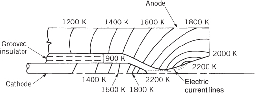
Figure 17–5 Simplified half‐section with an approximate typical temperature distribution in the electrodes of an arcjet.
Arcs are inherently unstable, often forming pinches and wiggles; they can only be stabilized with external electric fields and/or by swirling vortex motions at the outer gas layers. The arc‐current's flow configuration at the nozzle throat can be quite nonuniform and arc instabilities and erosion at the throat usually become life limiting. Proper mixing of cooler outer gas layers with arc‐heated inner gases tends to stabilize the arc while lowering its conductivity, which in turn requires higher voltages of operation. In some designs the arc is made longer by lengthening the throat.
The analysis of arcjets is based on plasma physics applied to a moving partially ionized fluid. Any conduction of electricity through a gaseous medium requires that a certain level of ionization be present. This ionization is obtained from an electrical discharge, that is, from the electric breakdown of the cold gas (resembling a lightning discharge in the atmosphere but, unlike it, a power supply feeds the current in either a continuous or pulsed fashion). Gaseous conductors of electricity follow a generalized version of Ohm's law; in an ordinary uniform medium where an electrical current ![]() is flowing across an area
is flowing across an area ![]() through a distance d by virtue of a voltage drop
through a distance d by virtue of a voltage drop ![]() , we may interpret Ohm's law (where
, we may interpret Ohm's law (where ![]() is the resistance) as
is the resistance) as
For the given uniform medium, we may define the electric field as ![]() , the current density as
, the current density as ![]() , and lastly introduce the electrical conductivity as
, and lastly introduce the electrical conductivity as ![]() . Thus, we may now rewrite the basic Ohm's law as simply
. Thus, we may now rewrite the basic Ohm's law as simply ![]() . The (scalar) electrical conductivity is directly proportional to the density of unattached or free electrons that, under equilibrium conditions, may be found from Saha's equation (Ref. 17–11). Strictly speaking, Saha's equation applies to thermal ionization only (and not necessarily to electrical discharges). For most gases, either high temperatures or low ionization energies or both are required for any useful ionization. However, since only about one free electron per million atoms/molecules is sufficient for workable conductivity levels, an inert gas may be “seeded” with low ionization potential vapors, as has been demonstrated in other plasmas. The magnitude of σ, the plasma's electrical conductivity, may be calculated based on the motion of free electrons from
. The (scalar) electrical conductivity is directly proportional to the density of unattached or free electrons that, under equilibrium conditions, may be found from Saha's equation (Ref. 17–11). Strictly speaking, Saha's equation applies to thermal ionization only (and not necessarily to electrical discharges). For most gases, either high temperatures or low ionization energies or both are required for any useful ionization. However, since only about one free electron per million atoms/molecules is sufficient for workable conductivity levels, an inert gas may be “seeded” with low ionization potential vapors, as has been demonstrated in other plasmas. The magnitude of σ, the plasma's electrical conductivity, may be calculated based on the motion of free electrons from
Here e is the electron charge, ![]() the free‐electron number density,
the free‐electron number density, ![]() a mean time between collisions, and
a mean time between collisions, and ![]() the electron mass.
the electron mass.
Actually, arc currents are nearly always influenced by magnetic fields, external or self‐induced, and a generalized Ohm's law (Ref. 17–12) for moving gases is needed, such as the following vector form (this equation is given in scalar forms in the section on electromagnetic devices):
The vector motion of the gas containing charged particles is represented by a velocity ![]() ; a magnetic induction field is given as
; a magnetic induction field is given as ![]() (a scalar B in the above equation is required in the last term) and an electric field as
(a scalar B in the above equation is required in the last term) and an electric field as ![]() . In Eq. 17–12, both the current density
. In Eq. 17–12, both the current density ![]() and the conductivity are understood to relate only to the free electrons as does
and the conductivity are understood to relate only to the free electrons as does ![]() , the Hall parameter. This Hall parameter consists of the electron cyclotron frequency (
, the Hall parameter. This Hall parameter consists of the electron cyclotron frequency (![]() ) multiplied by the mean time it takes an electron to lose its momentum by collisions with the heavier particles (
) multiplied by the mean time it takes an electron to lose its momentum by collisions with the heavier particles (![]() ). The second term in Eq. 17–12 (
). The second term in Eq. 17–12 (![]() ) is the induced electric field due to any plasma motion normal to the magnetic field, and the last term represents the Hall electric field which is perpendicular to both the current vector and the applied magnetic field vector as the cross product (i.e., the “×”) implies (for simplicity ionslip and electron pressure gradients have been omitted here). Magnetic fields are responsible for most of the peculiarities observed in arc behavior, such as pinching (a constriction arising from the current interacting with its own magnetic field), and play a central role in nonthermal electromagnetic types of thrusters, as discussed in a following section.
) is the induced electric field due to any plasma motion normal to the magnetic field, and the last term represents the Hall electric field which is perpendicular to both the current vector and the applied magnetic field vector as the cross product (i.e., the “×”) implies (for simplicity ionslip and electron pressure gradients have been omitted here). Magnetic fields are responsible for most of the peculiarities observed in arc behavior, such as pinching (a constriction arising from the current interacting with its own magnetic field), and play a central role in nonthermal electromagnetic types of thrusters, as discussed in a following section.
To initiate an arcjet, a much higher voltage than necessary for operation needs to be momentarily applied in order to ‘break down’ the cold gas to produce a plasma. Some arcjets require an extended initial burn‐in period before consistent running ensues. Because the conduction of electricity through a gas is inherently unstable, arcs use a conventional external or ‘ballast’ resistance to allow steady‐state operation. The cathode must run hot and is usually made of tungsten with 1 or 2% thorium (suitable up to about 3000 K). Boron nitride, an easily shaped high‐temperature electrical insulator, is commonly used.
Presently, most arcjets are rather inefficient since less than half of the electrical energy goes into kinetic energy of the jet; the nonkinetic part of the exhaust plume (residual internal energy and ionization) is the largest loss. About 10 to 20% of the electric power input is usually dissipated and radiated as heat to space or transferred by conduction from the hot nozzle to other parts of the system. Arcjets, however, are potentially scalable to larger thrust levels than any other electric propulsion systems. Generally, arcjets exhibit about one‐sixth the thrust‐to‐power ratio of resistojets because of their increased specific impulse coupled with relatively low values of efficiency. Moreover, arcjets have another disadvantage in that the required power processing units need to be more complex than those for resistojets due to the intricacy of arc phenomena.
The life of an arcjet is often severely limited by electrode erosion and vaporization, which arise at the arc attachment or foot‐point, and because of the high operating temperatures in general. The rate of erosion is influenced by the particular propellant in combination with the electrode materials (argon and nitrogen give higher erosion rates than hydrogen), and by pressure gradients, which are much higher during start or pulsing transients (often by a factor of 100) than during steady‐state operation. A variety of propellants have been used in arcjet devices, but the industry has now settled on the catalytic decomposition products of hydrazine (![]() ); see Section 7.4.
); see Section 7.4.
An arcjet downstream from a catalytic hydrazine decomposition chamber looks similar to the resistojet of Fig. 17–4, except that the resistor is replaced by a smaller diameter chamber where an arc heats the gases, see Fig. 17–6. Also, larger cables are needed to supply the higher operating currents. Decomposed hydrazine would enter the arc at a temperature of about 760 °C. Liquid hydrazine is relatively storable and provides a low‐volume, light‐weight propellant supply system when compared to gaseous propellants, but its use requires appropriate thermal control of tanks to prevent freezing and thermal tank isolation to prevent detonations from hydrazine overheated by external sources. Table 17–4 shows on‐orbit performance of a system of a 2‐kW hydrazine arcjet used for N‐S‐stationkeeping. Specific impulses range up to 600 sec for hydrazine arcjets (Ref. 17–13). A 30‐kW ammonia arcjet program (ESEX) flew in 1999 (Ref. 17–14) with 786 sec specific impulse and 2 N thrust. NASA and NOAA presently operate hydrazine arcjet thrusters in the GOES‐R spacecraft with an Is of 600 sec. The performance of hydrazine augmented arcjets is roughly twice that of hydrazine resitojets.
Table 17–4 On‐Orbit Data for the 2‐kW MR‐510 Hydrazine Arcjet System
Source: From Ref 26.
| Propellant | Hydrazine |
| Steady thrust | 222–258 mN |
| Mass flow rate | 40 mg/sec |
| Feed pressure | 200–260 psia |
| Power control unit (PCU) input | 4.4 kW (two thrusters) |
| System input voltage | 70 V DC |
| PCU efficiency | 91% |
| Specific impulse | 570–600 sec |
| Dimensions | |
| Arcjet (approx.) | 237 × 125 × 91 mm3 |
| PCU | 631 × 359 × 108 mm3 |
| Mass | |
| Arcjet (4) and cable | 6.3 kg |
| PCU | 15.8 kg |
| Total impulse | 1,450,900 N‐sec |

Figure 17–6 Perspective drawing of a 2‐kW arcjet thruster. Its performance is initially augmented by the catalytic‐decomposition of hydrazine into moderately hot gases, which are in turn fed through an electric arc and further heated. The arc is located at the centerline of the flow passage at the throat region of a converging‐diverging nozzle.
Courtesy of Aerojet Rocketdyne, Redmond Operations
17.3 NONTHERMAL ELECTRICAL THRUSTERS
The acceleration of hot propellant gases using a supersonic nozzle is the most conspicuous feature of thermal thrusting. Now we turn our study to propellant acceleration by electrical forces where no enclosure area changes are essential for direct gas acceleration. Electrostatic (or Coulomb) forces and electromagnetic (or Lorentz) forces can accelerate a suitably ionized propellant to speeds ultimately limited by the speed of light (note that thermal thrusting is essentially limited by the speed of sound in the plenum chamber). The microscopic vector force ![]() on a singly charged particle may be written as
on a singly charged particle may be written as
where ![]() is the electron charge magnitude,
is the electron charge magnitude, ![]() the electric field vector,
the electric field vector, ![]() the velocity of the charged particle, and
the velocity of the charged particle, and ![]() the magnetic field vector. Summing these electromagnetic forces on all charges gives the total force per unit volume vector
the magnetic field vector. Summing these electromagnetic forces on all charges gives the total force per unit volume vector ![]() (scalar forms of this equation follow):
(scalar forms of this equation follow):
Here ![]() is the net charge density and
is the net charge density and ![]() the vector electric current density. With plasmas, which by definition have an equal mixture of positively and negatively charged particles within a volume of interest, this net charge density vanishes. On the other hand, the current due to an electric field does not vanish in plasmas because positive ions move opposite to electrons, thus adding to the current (but in plasmas with free electrons this ion current is very small). From Eq. 17–14, we can surmise that an electrostatic accelerator should have a nonzero net charge density, commonly referred to as the space–charge density. A common electrostatic accelerator is the ion thruster, which operates with positive ions; here magnetic fields are unimportant in the accelerator region. Electromagnetic accelerators (e.g., the MPD and PPT) operating only with plasmas rely solely on the Lorentz force to accelerate the propellant. The Hall accelerator may be thought of as a crosslink between ion and electromagnetic thrusters. These three types of accelerator are discussed next. Presently, extensive research and development efforts with nonthermal thrusters continue to be truly international.
the vector electric current density. With plasmas, which by definition have an equal mixture of positively and negatively charged particles within a volume of interest, this net charge density vanishes. On the other hand, the current due to an electric field does not vanish in plasmas because positive ions move opposite to electrons, thus adding to the current (but in plasmas with free electrons this ion current is very small). From Eq. 17–14, we can surmise that an electrostatic accelerator should have a nonzero net charge density, commonly referred to as the space–charge density. A common electrostatic accelerator is the ion thruster, which operates with positive ions; here magnetic fields are unimportant in the accelerator region. Electromagnetic accelerators (e.g., the MPD and PPT) operating only with plasmas rely solely on the Lorentz force to accelerate the propellant. The Hall accelerator may be thought of as a crosslink between ion and electromagnetic thrusters. These three types of accelerator are discussed next. Presently, extensive research and development efforts with nonthermal thrusters continue to be truly international.
Analyses of electrostatic and electromagnetic thruster are based on the basic laws of electricity and magnetism which are found in Maxwell's equations complemented by the electromagnetic force relation (Eq. 17–14) and the generalized Ohm's law (Eq. 17–12). In addition, various phenomena peculiar to ionization and to gaseous conduction need to be considered. These subjects form the basis of the discipline of magnetohydrodynamics or MHD, a proper treatment of which is beyond the scope of this book.
Electrostatic Devices
Electrostatic thrusters rely on Coulomb forces to accelerate propellant gases comprised of nonneutral charged particles. They operate only in a near vacuum where internal particle collisions are few. The electric force is proportional to the space charge density; since all charged particles are of the same “sign,” they move in the same direction. Electrons are easy to produce and readily accelerated, but their extremely light mass makes them impractical for electric propulsion. From thermal propulsion fundamentals (see Chapter 3) we showed that “the lighter the exhaust particle the better.” However, the momentum carried by electrons is relatively negligible even at nonrelativistic high velocities, and the thrust per unit area derived from any electron flow remains negligible even when the effective exhaust velocity or specific impulse is high (see Problem 17–11). Accordingly, electrostatic thrusters use singly charged high‐molecular‐mass atoms as positive ions (a proton has 1836 times the mass of the electron and typical ions of interest contain hundreds of proton‐equivalent particles). There has been some research work with tiny liquid droplets or charged colloids which can in turn be some 10,000 times more massive than atomic particles. In terms of power sources and internal equipment, the use of colloids permits more desirable characteristics for electrostatic thrusters—for example, high voltages and low currents in contrast to the conventional low voltages and high currents with their associated massive wiring and switching requirements.
Electrostatic (ion) thrusters may be categorized by the charged particle source. Note that exit beam neutralization is required in all these schemes.
- Electron bombardment thrusters. Positive ions are produced by bombarding a gas or vapor, such as xenon or mercury, with electrons usually emitted from a heated cathode in a suitable plenum chamber. Ionization voltages can be either DC or RF. In these ion thrusters (see Fig. 1–9), acceleration is accomplished with a separate electrical source applied through a series of suitably manufactured and positioned electrically conducting grids. This method is the oldest and presently the most common.
- Field emission thrusters. With the field emission electric propulsion (FEEP) concept, positive ions are obtained from a liquid metal source flowing through capillary tubes and several geometrical arrangements are possible (Ref. 17–15). Liquid metals such as indium (Ref. 17–16) or cesium when subjected to high enough electric fields
 produce molecular ions that flow into an accelerating region. The injector, ionizer, and accelerator are all part of the same voltage circuit which operates typically at values over 10 kV;
  values are around 8000 to 9000 sec. This is a robust concept being considered for micropropulsion (thrust levels below 1 mN, Ref. 17–1) applications. Some FEEPs have been space qualified.
 - Colloids. Here charged liquid droplets produced by an electrospray (or field evaporation process) are used. The propellants are typically liquid metals (or low volatility ionic liquids). These are presently under development and also of interest for micropropulsion, Ref. 17–1.
Examples of space flights where electrostatic units have provided the primary propulsion are the NSTAR (a DC‐electron‐bombardment xenon ion thruster, Refs. 6 and 34) used in NASA's DS1 and the ongoing DAWN missions, and RITA (radio frequency ion thrusters) flown in several European missions and Japan's Hayabusa spacecraft with four microwave ion engines is another mission which included landing and taking off from an asteroid, Refs. 6 and 36. Boeing has extensively used “L‐3 Communications” XIPS 25‐cm ion thruster in its geosynchronous communications satellites.
Basic Relationships for Electrostatic Thrusters
An electrostatic thruster, regardless of type, consists of the same series of basic ingredients, namely, a propellant source, several forms of electric power, an ionizing chamber, an accelerator region, and a means of neutralizing the exhaust (see Fig. 1–9). While all Coulomb‐force accelerators require a net charge density of unipolar ions, the exhaust beam must be neutralized to avoid a space–charge buildup outside of the craft, which easily nullifies the operation of the thruster. Neutralization is achieved by the injection of electrons downstream of the accelerator. The ion exhaust velocity is a function of the voltage ![]() imposed across an accelerating chamber consisting of ion‐permeable grids, and the mass of the charged particle
imposed across an accelerating chamber consisting of ion‐permeable grids, and the mass of the charged particle ![]() of electrical charge
of electrical charge ![]() . In the conservation of energy equation the kinetic energy of a charged particle must equal the electrical energy gained from the field, provided that there are no collisional or other losses. For charges injected with a velocity
. In the conservation of energy equation the kinetic energy of a charged particle must equal the electrical energy gained from the field, provided that there are no collisional or other losses. For charges injected with a velocity ![]() ,
,
This equation describes one‐dimensional transit along the accelerator coordinate ![]() . The total ion speed issuing from the accelerator becomes,
. The total ion speed issuing from the accelerator becomes,
When ![]() is ion charge in coulombs,
is ion charge in coulombs, ![]() is the ion mass in kilograms, and
is the ion mass in kilograms, and ![]() is in volts, then v is in meters per second. Using
is in volts, then v is in meters per second. Using ![]() to represent the molecular mass of the ion
to represent the molecular mass of the ion ![]() kg/kg‐mole for a proton), then, for singly charged ions, the equation above becomes
kg/kg‐mole for a proton), then, for singly charged ions, the equation above becomes ![]() when
when ![]() may be neglected. References 17–3 and 17–4 contain more detailed treatments of the applicable theory.
may be neglected. References 17–3 and 17–4 contain more detailed treatments of the applicable theory.
In an ideal ion thruster, the electric current ![]() across the accelerator consists of all the propellant mass flow rate (fully but singly ionized and purely unidirectional), i.e.,
across the accelerator consists of all the propellant mass flow rate (fully but singly ionized and purely unidirectional), i.e.,
The total ideal thrust from the accelerated particles is given by Eq.2–13 (without the pressure thrust term, as gas pressures are extremely low):
For a given current and accelerator voltage, the thrust is proportional to the mass‐to‐charge ratio (![]() ) of the charged particles and high molecular mass ions are favored because they yield high thrust per unit volume. Both the thrust and the power absorbed by the electrons in the neutralizing region are small (about 1%) and can thus be neglected.
) of the charged particles and high molecular mass ions are favored because they yield high thrust per unit volume. Both the thrust and the power absorbed by the electrons in the neutralizing region are small (about 1%) and can thus be neglected.
The current density ![]() that can flow within a nonneutral charged particle beam has a theoretical limit (unconnected to any source‐current saturation) which depends on the beam's geometry and on the voltage applied (see Refs. and 38). This fundamental constraint is caused by an internal electric field associated with the ion cloud that opposes the imposed electric field so that only a certain maximum number of charges of the same sign can pass simultaneously through the accelerator region. This space‐charge limited current is found from Poisson's equation as traditionally applied to a one‐dimensional planar electrode region. We next define of the current density in terms of the space–charge density (
that can flow within a nonneutral charged particle beam has a theoretical limit (unconnected to any source‐current saturation) which depends on the beam's geometry and on the voltage applied (see Refs. and 38). This fundamental constraint is caused by an internal electric field associated with the ion cloud that opposes the imposed electric field so that only a certain maximum number of charges of the same sign can pass simultaneously through the accelerator region. This space‐charge limited current is found from Poisson's equation as traditionally applied to a one‐dimensional planar electrode region. We next define of the current density in terms of the space–charge density (![]() ) as:
) as:
Injection velocities can never be zero, but when the injected charges have a negligible kinetic energy compared to that gained within the accelerator operating at ![]() , (i.e., dropping out
, (i.e., dropping out ![]() ), it is possible to solve Eqs. 17–19, and 17–20 directly and obtain the classic relation known as Child–Langmuir's law:
), it is possible to solve Eqs. 17–19, and 17–20 directly and obtain the classic relation known as Child–Langmuir's law:
Otherwise, when the injected ion kinetic energy is sufficiently large relative to the energy gained in the accelerator, Eq. 17–16 remains unmodified and an enhanced current beyond its Child‐Langmuir value may result. As long as the current emitted from the source has not saturated, analysis shows that the current increase may be as high as ![]() , given below as Eq.17–21 (where
, given below as Eq.17–21 (where ![]() is the ratio of the initial ion energy to the energy gained in the accelerator, assuming monoenergetic beam injection), see Ref. 17–20,
is the ratio of the initial ion energy to the energy gained in the accelerator, assuming monoenergetic beam injection), see Ref. 17–20,
Returning now to Eq. 17–20 where ![]() , d represents the accelerator interelectrode distance and ε0 the permittivity of free space which, in SI units, becomes 8.854 × 10⁻¹² farads/meter. In SI units Eq. 17–20, the classical saturation current density may be expressed (for atomic or molecular ions) as
, d represents the accelerator interelectrode distance and ε0 the permittivity of free space which, in SI units, becomes 8.854 × 10⁻¹² farads/meter. In SI units Eq. 17–20, the classical saturation current density may be expressed (for atomic or molecular ions) as
Here the current density is in A/m2, the voltage is in volts, and the distance in meters. For xenon with electron bombardment ionization, values of j vary from 2 to about 10 mA/cm2. In practice, acceleration is seldom one‐dimensional and the current density and cross sectional area depend on accelerator voltage as well as on electrode configuration and spacing.
Using Eqs. 17–18 (with ![]() ) and 17–22 and letting the beam cross section be circular so that the current through each grid hole (see Fig. 17–7) becomes
) and 17–22 and letting the beam cross section be circular so that the current through each grid hole (see Fig. 17–7) becomes ![]() , the corresponding thrust may be rewritten as
, the corresponding thrust may be rewritten as
In SI units, this classical space‐charge limited relation becomes

Figure 17–7 Simplified schematic diagram of an electron bombardment ion thruster showing, enlarged, a two‐screen accelerator grid section. Presently thrusters use a three‐grid acceleration unit and permanent magnets instead of coils.
The ratio of a beam's diameter ![]() to the accelerator–electrode grid spacing
to the accelerator–electrode grid spacing ![]() is regarded as an aspect ratio for the ion accelerator region. For multiple grids with equal holes (see Figs. 17–7 and 17–8) the diameter
is regarded as an aspect ratio for the ion accelerator region. For multiple grids with equal holes (see Figs. 17–7 and 17–8) the diameter ![]() is that of the individual perforation hole and the distance d is the mean spacing between grids. Because of space–charge limitations,
is that of the individual perforation hole and the distance d is the mean spacing between grids. Because of space–charge limitations, ![]() can have values no higher than about one for simple, single‐ion beams. This implies a rather stubby thruster design with many perforations and the need for large numbers or multiple parallel ion beamlets for high thrust requirements, but other practical considerations also need to be considered.
can have values no higher than about one for simple, single‐ion beams. This implies a rather stubby thruster design with many perforations and the need for large numbers or multiple parallel ion beamlets for high thrust requirements, but other practical considerations also need to be considered.

Figure 17–8 External view and section of a 500‐watt ion propulsion system (XIPS), rated at 18 mN and 2800 sec. Also shown are hollow‐cathodes for ionization and for beam neutralization. Xenon gas is delivered to the ionizer, then accelerated through the extraction electrodes with an added “screen electrode,” after this section the ion beam is neutralized.
Drawing courtesy of L‐3 Communications Electron Technologies, Inc., and the American Physical Society
Using Eqs. 17–1, 17–2, and 17–17, and allowing for losses in the conversion of potential energy to kinetic energy, the power needed for the electrostatic accelerator region becomes
Here, the electrostatic thruster efficiency (![]() ) is part of the overall thruster efficiency
) is part of the overall thruster efficiency ![]() (see Eq. 17–2) and among other losses includes the ionization‐energy expenditure. Ionization energies represent an input necessary to make the propellant respond to the electrostatic force and are nonrecoverable. The ionization energy is found from the ionization potential (
(see Eq. 17–2) and among other losses includes the ionization‐energy expenditure. Ionization energies represent an input necessary to make the propellant respond to the electrostatic force and are nonrecoverable. The ionization energy is found from the ionization potential (![]() ) of the atom or molecule times the current flow, as the Example 17–2 demonstrates. Table 17–5 shows molecular masses and ionization potentials for different gaseous propellants. In actual practice, considerably higher voltages than the ionization potential are required to operate the ionization chamber.
) of the atom or molecule times the current flow, as the Example 17–2 demonstrates. Table 17–5 shows molecular masses and ionization potentials for different gaseous propellants. In actual practice, considerably higher voltages than the ionization potential are required to operate the ionization chamber.
Table 17–5 Ionization Potentials for Various Gases
| Gas | Ionization Potential (eV) | Molecular or Atomic Mass (kg/kg‐mol) |
| Cesium vapor | 3.9 | 132.9 |
| Bismuth | 7.3 | 209 |
| Mercury vapor | 10.4 | 200.59 |
| Xenon | 12.08 | 131.30 |
| Krypton | 14.0 | 83.80 |
| Hydrogen, molecular | 15.4 | 2.014 |
| Argon | 15.8 | 39.948 |
Ionization Schemes
Ordinary gaseous propellants must be ionized before they can be electrostatically accelerated. Even though all ion acceleration schemes are fundamentally the same, several ionization schemes are available. Most devices ionize using direct current discharges (DC) but some use high‐frequency alternating currents (RF). The ionization chamber is responsible for most of the size, mass, and internal efficiency of these thrusters.
Ionization of a gas by electron bombardment is a well‐established technology (Refs. and 38). Electrons emitted from a thermionic (hot) cathode or the more efficient “hollow cathode” are made to interact with a gaseous propellant flow inside a suitable ionization chamber. The chamber pressures are low, about 10−3 torr or 0.134 Pa. Figure 17–7 depicts a typical electron‐bombardment ionizer, which contains neutral atoms, positive ions, and electrons. Emitted electrons, attracted toward the chamber's cylindrical anode, are forced to spiral by the axial magnetic field, thus enabling the numerous collisions with propellant atoms needed for ionization; the more contemporary devices incorporate “ring‐cusp magnetic circuits,” which rely on a “magnetic mirror effect” to control and filter the discharge electrons. A radial electric field removes electrons from the chamber and an axial electric field moves positive ions toward the accelerator grids. These grids are designed to act as “porous electrodes,” where only the positive ions are accelerated. Electrons losses are minimized by maintaining the cathode potential negatively biased at both the inner grid electrode and at the opposite wall of the chamber. An external circuit routs the extracted electrons from the cylindrical anode and re‐introduces them at the exhaust beam in order to neutralize it.
Figure 17–8 shows the cross section of a xenon ion propulsion thruster with three perforated electrically charged grids or ‘ion extraction electrodes’. Here the inner one is charged to the cathode potential (typically 1000 V with respect to the spacecraft ground plasma potential), the second or ‘accelerator electrode’ is typically charged to – 200 V, and the third or ‘decelerator electrode’ is tied to the neutralizer (so as to reduce sputter‐eroded products and to improve the beam focusing in the near field). Hence the saturation current density is given the potential difference between the first two electrodes and the extraction velocity is given by the potential difference between the screen and accelerator electrodes. Each grid hole is suitably aligned with a similar opening in other grids and the ion beamlets flow through these holes.
Other key thruster components are (1) cathode heaters, (2) a propellant feed system, (3) electrical insulators, and (4) permanent magnets. Reference 17–17 describes a 500‐W xenon thruster. Hollow cathodes are efficient electron emitters but, because of their size and complexity, carbon‐nanotube electron‐field emitters are presently being explored. Xenon, the highest molecular mass stable inert gas, has been the propellant of choice. Xenon is a minor component of air, in a concentration of about 9 parts in 100 million, so it is relatively rare and expensive. It is easily stored below its critical temperature as a liquid and does not pose any problems of condensation or toxicity. Pressure regulators for xenon need to be quite sophisticated because no leakages can be tolerated as flows are quite small.
Electromagnetic Thrusters
This third category of electric propulsion devices accelerates propellant gases that have been heated up to a plasma state. Plasmas are neutral mixtures of electrons and positive ions (often including un‐ionized atoms/molecules) that can readily conduct electricity, existing at temperatures usually above 5000 K or 9000 °R. According to electromagnetic theory, whenever a conductor carries a current perpendicular to a magnetic field, a body force is exerted on that conductor in a direction at right angles to both the current and the magnetic field. Unlike the ion thruster, this acceleration process yields a neutral exhaust beam. Another advantage is the relatively high thrust density, or thrust per unit area, which can be 10 to 100 times that of electrostatic thrusters.
Basically, designs of electromagnetic thrusters consist of a region of electrically conductive gas where a high current produced by an applied electric field accelerates the propellant though the action of either an external or a self‐generated magnetic field. Many conceptual arrangements have undergone laboratory study, some with external and some with self‐generated magnetic fields, some suited to continuous thrusting and some limited to pulsed thrusting. Table 17–6 shows ways in which electromagnetic thrusters are categorized. Because there is a wide variety of devices with a correspondingly wide array of names, we will use the term Lorentz‐force accelerators when referring to their principle of operation. For all of these devices the plasma current must be part of the electrical circuit and most accelerator geometries are constant area. Motion of the propellant, a moderate‐density plasma—usually a combination of ionized and cooler gas particles, is due to a complex set of interactions. This is particularly true of short duration (3 to ![]() ) pulsed‐plasma thrusters where nothing reaches a thermal equilibrium state.
) pulsed‐plasma thrusters where nothing reaches a thermal equilibrium state.
Table 17–6 Characterization of Electromagnetic Thrusters
| Thrust Mode | ||
| Steady State | Pulsed (Transient) | |
| Magnetic field source | External coils or permanent magnets | Self‐induced |
| Electric current source | Direct‐current supply | Capacitor bank and fast switches |
| Working fluid | Pure gas, mixtures, seeded gas, or vaporized liquid | Pure gas or stored as solid |
| Geometry of path of working fluid | Axisymmetric (coaxial) rectangular, cylindrical, constant or variable cross section | Ablating plug, axisymmetric, other |
| Special features | Using Hall current or Faraday current | Simple requirement for propellant storage |
Conventional Thrusters—MPD and PPT
Any description of magneto‐plasma‐dynamic (MPD) and pulsed‐plasma (PPT) electromagnetic thrusters is based on plasma conduction in the direction of the applied electric field but perpendicular to the magnetic field, with both of these vectors in turn normal to the direction of plasma acceleration (see Ref. 17–12). Equation 17–12 may be specialized here to a Cartesian coordinate system where the plasma's “mass‐mean velocity” is in the x direction, the external electric field is in the y direction (![]() ), and the magnetic field acts in the z direction (
), and the magnetic field acts in the z direction (![]() ). A simple manipulation of Eq. 17–12, with negligible Hall parameter
). A simple manipulation of Eq. 17–12, with negligible Hall parameter ![]() , yields a scalar equation for the current, noting that only
, yields a scalar equation for the current, noting that only ![]() (termed the Faraday current),
(termed the Faraday current), ![]() , and
, and ![]() remain present:
remain present:
and the Lorentz force (from Eq. 17–14) becomes
Here ![]() represents the force “density” within the accelerator and should not be confused with F the total thrust force;
represents the force “density” within the accelerator and should not be confused with F the total thrust force; ![]() has units of force per unit volume (e.g., N/m3). The axial velocity
has units of force per unit volume (e.g., N/m3). The axial velocity ![]() is a mass‐mean velocity that increases internally along the accelerator length; the actual thrust equals the exit value (
is a mass‐mean velocity that increases internally along the accelerator length; the actual thrust equals the exit value (![]() or
or ![]() ) multiplied by the mass flow rate. It is noteworthy that, as long as
) multiplied by the mass flow rate. It is noteworthy that, as long as ![]() and
and ![]() (or
(or ![]() ) remain somewhat constant, both the current and the force decrease along the accelerator length due to the induced field
) remain somewhat constant, both the current and the force decrease along the accelerator length due to the induced field ![]() , which subtracts from the impressed value
, which subtracts from the impressed value ![]() . Such plasma velocity behavior translates into a diminishing force along Faraday accelerators, with eventual limits on the final axial velocity. Although not practical, it would seem desirable to design for increasing E/B along the channel in order to maintain substantial accelerating forces throughout. But it is not necessarily of interest to design for peak exit velocities because these might translate into unrealistically long accelerators (see Problem 17–8). It can be shown that practical considerations would restrict these exit velocities to below one‐tenth of the maximum value of
. Such plasma velocity behavior translates into a diminishing force along Faraday accelerators, with eventual limits on the final axial velocity. Although not practical, it would seem desirable to design for increasing E/B along the channel in order to maintain substantial accelerating forces throughout. But it is not necessarily of interest to design for peak exit velocities because these might translate into unrealistically long accelerators (see Problem 17–8). It can be shown that practical considerations would restrict these exit velocities to below one‐tenth of the maximum value of ![]() .
.
A “gas‐dynamic approximation” (essentially an extension of the classical concepts of Chapter 3 to plasmas in electromagnetic fields) by Resler and Sears (Ref. 17–21) indicates that further complications are possible, namely, that a constant area accelerator channel would choke if the plasma velocity does not have the very specific value of ![]() at the sonic location of the accelerator. This plasma tunnel velocity would have to be equal to 40% of the value of
at the sonic location of the accelerator. This plasma tunnel velocity would have to be equal to 40% of the value of ![]() for inert gases, since
for inert gases, since ![]() (their ratio of specific heats) equals 1–67. Thus, constant area, constant
(their ratio of specific heats) equals 1–67. Thus, constant area, constant ![]() accelerators could be severely constrained because Mach 1 corresponds only to about 1000 m/sec in typical inert gas plasmas; constant‐area choking in real systems, where the properties
accelerators could be severely constrained because Mach 1 corresponds only to about 1000 m/sec in typical inert gas plasmas; constant‐area choking in real systems, where the properties ![]() ,
, ![]() , and
, and ![]() are actually quite variable, is more likely to manifest itself as one or more instabilities. Another problem here is that values of the conductivity and electric field are usually difficult to determine and a combination of analysis and measurement is often required to evaluate, for example, Eq. 17–12. Fortunately, most plasmas are reasonably good conductors even when less than 10% of the gas particles are ionized.
are actually quite variable, is more likely to manifest itself as one or more instabilities. Another problem here is that values of the conductivity and electric field are usually difficult to determine and a combination of analysis and measurement is often required to evaluate, for example, Eq. 17–12. Fortunately, most plasmas are reasonably good conductors even when less than 10% of the gas particles are ionized.
Figure 17–9 shows the simplest plasma accelerator, which employs a self‐induced magnetic field. This is the pulsed plasma thruster (PPT) where an accelerating plasma burst or “bit,” created by a spark discharge between the accelerator electrodes, is powered by a capacitor, which in turn is charged from the spacecraft's power supply. The flow of current through the plasma rapidly discharges the capacitor and hence such mass‐flow‐rate pulse must be synchronized with a “discharge schedule.” The discharge current closes a “current loop,” one which induces a significant magnetic field perpendicular to the plane of the rails. Analogous to a metal conductor in an electric motor, the Lorentz force acts on the movable plasma segment, accelerating it along the rails. Hence, no area changes (i.e., nozzles) are necessary to accelerate the propellant.
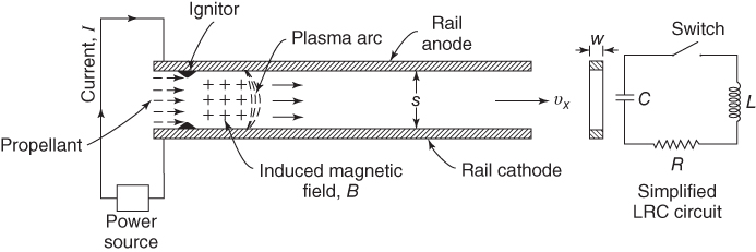
Figure 17–9 Simple rail accelerator for self‐induced magnetic field acceleration of current‐carrying plasma. This concept illustrates the basic physical interactions; it suffers from propellant losses, resulting in low efficiencies.

Figure 17–10 Simplified diagram of a magnetoplasma dynamic (MPD) arcjet thruster. Similar in construction to the thermal arcjet shown in Fig. 1–8, it has a strong magnetic field to produce propellant acceleration.
As indicated in Fig. 17–9, the system (though containing a plasma along with other more ordinary resistances) may be modeled with an equivalent L‐R‐C pulsed circuit where ![]() is the lumped‐parameter total circuit inductance, R is the total Ohmic resistance, and
is the lumped‐parameter total circuit inductance, R is the total Ohmic resistance, and ![]() is an effective capacitance. It is undesirable to let the current reverse during each pulsing as this diminishes the overall thrust; a nonoscillatory pulse may be realized through the
is an effective capacitance. It is undesirable to let the current reverse during each pulsing as this diminishes the overall thrust; a nonoscillatory pulse may be realized through the ![]() “impedance‐balancing criterion” (when this is not physically possible, a “quenching diode” is inserted, see Ref. 17–22). In some designs, the hot plasma pulse has sufficient gas‐dynamic expansion capabilities to contribute to the thrust (needing the addition a nozzle for thermal expansion). In many typical configurations, the rate of increase of circuit inductance with the distance the arc travels (
“impedance‐balancing criterion” (when this is not physically possible, a “quenching diode” is inserted, see Ref. 17–22). In some designs, the hot plasma pulse has sufficient gas‐dynamic expansion capabilities to contribute to the thrust (needing the addition a nozzle for thermal expansion). In many typical configurations, the rate of increase of circuit inductance with the distance the arc travels (![]() ) is the sole propulsive contributor
) is the sole propulsive contributor ![]() where
where ![]() is the current in the loop); since the induced magnetic field is a function of accelerator geometry, the axial thrust obtained may be written for the two configurations listed below as
is the current in the loop); since the induced magnetic field is a function of accelerator geometry, the axial thrust obtained may be written for the two configurations listed below as
The linear rail spacing is s and the rail width is ![]() as shown in Fig. 17–9; for the coaxial accelerator the equation above describes an electrode geometry of inner radius
as shown in Fig. 17–9; for the coaxial accelerator the equation above describes an electrode geometry of inner radius ![]() and constant outer radius
and constant outer radius ![]() (space qualification for the coaxial micro‐PPT has not been reported to date). Because plasmas are nonmagnetic, the value of
(space qualification for the coaxial micro‐PPT has not been reported to date). Because plasmas are nonmagnetic, the value of ![]() remains the same as free space, namely,
remains the same as free space, namely, ![]() .
.
A practical first version of the PPT that flew in 1968 is shown in Chapter 1 as Fig. 1–10. The propellant is stored as a solid Teflon bar that is pushed by a spring against two linear rails where a pulsed discharge is initiated across surface momentarily ablating a small portion of propellant. Teflon stores well in space, is easy to handle, and ablates without significant charring. There are no tanks, valves, synchronizing controls, or zero gravity feed requirements. A rechargeable capacitor fed from a power processing unit in the spacecraft provides the power input. Thrust results only as rapid pulses unlike most other electric propulsion devices; these pulsed thrusters are very compatible with precise control and positioning maneuvers where mean thrust can be varied by changing the pulsing rate or the total number of pulses ![]() . If a “total impulse per pulse” or impulse bit (in units of N‐sec or lbf‐sec) is denoted by
. If a “total impulse per pulse” or impulse bit (in units of N‐sec or lbf‐sec) is denoted by ![]() , then the overall vehicle change of velocity
, then the overall vehicle change of velocity ![]() would be the sum of N tiny but equal pulses; using Eqs. 2–4 and 4–6 a much simplified result equivalent to Eq. 4–36 may be obtained provided that
would be the sum of N tiny but equal pulses; using Eqs. 2–4 and 4–6 a much simplified result equivalent to Eq. 4–36 may be obtained provided that ![]() where cm0 is the product of the effective exhaust velocity
where cm0 is the product of the effective exhaust velocity ![]() with the initial mass, as would relate to the PPT:
with the initial mass, as would relate to the PPT:
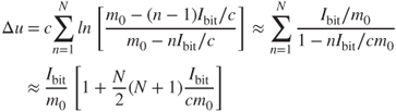
Much electrical energy is lost in PPT circuits on top of the ionization energy, which cannot be recovered; moreover, the bits of mass being accelerated do not typically exit well collimated and propellant utilization has been poor in earlier designs. Besides its very low efficiency, a disadvantage of the PPT has been the size and mass of the early capacitors and associated power conditioning equipment. Interest in PPTs has been renewed for micropropulsion (small satellite propulsion) using better designs.
Figure 17–10 shows a hybrid electrothermal–electromagnetic arcjet concept, which is of interest because unlike the PPT it has a high‐thrust capability. It can produce continuous large thrusts and Russia and Japan have flown some versions. Compared to electrothermal arcjets, these devices operate at relatively lower propellant pressures and much higher electric and magnetic fields. Hydrogen and argon are common propellants used for such MPD arcjets. Unlike ion thrusters, exhaust beam neutralization is unnecessary. Problems of high electrode erosion, massive electrical components, and low efficiencies (with their associated heat dissipation needs) have slowed implementation of these devices, which also depend on relatively large, more complex, and expensive quantities of electric power.
Hall‐Effect Thrusters
When plasma densities are low enough and/or magnetic fields sufficiently high, the Hall‐effect electric field becomes significant. This is the same phenomenon that is observed as the semiconductor Hall effect where a voltage appears transverse to the applied electric field. Hall currents can be understood to represent the motion of an electron “guiding center” (Ref. 17–11) in a crossed electric and magnetic field arrangement where electron collisions must be relatively insignificant. Hall thrusters are of interest because they represent a very practical operating region for space propulsion. Russian scientists were the first to successfully deploy them in many vehicles, a design originally called the stationary plasma thruster or SPT. Hall thrusters are described in Ref. 17–3.
In order to understand the Hall thruster principle, it is necessary to rewrite in scalar form the generalized Ohm's law, Eq. 17–12. Because the electron Hall parameter ![]() (introduced in Eq. 17–12 and described below Eq. 17–34) is no longer negligible, we arrive at two equations (shown in Cartesian form):
(introduced in Eq. 17–12 and described below Eq. 17–34) is no longer negligible, we arrive at two equations (shown in Cartesian form):
In typical designs, imposing a longitudinal electric field ![]() causes a current density
causes a current density ![]() to flow in the applied field direction together with a Hall current density
to flow in the applied field direction together with a Hall current density ![]() which flows in the direction transverse to
which flows in the direction transverse to ![]() . The associated induced Hall electric field
. The associated induced Hall electric field ![]() is externally shorted to maximize the Hall current, and the electrodes are “segmented” in order not to short out the axial electric field
is externally shorted to maximize the Hall current, and the electrodes are “segmented” in order not to short out the axial electric field ![]() . It is necessary that
. It is necessary that ![]() . Such arrangement unavoidably results in a very complicated design. For space propulsion, engineers prefer the cylindrical geometry because it yields a simpler, more practical design; here the applied magnetic field (
. Such arrangement unavoidably results in a very complicated design. For space propulsion, engineers prefer the cylindrical geometry because it yields a simpler, more practical design; here the applied magnetic field (![]() ) is radial and the applied electric field is axial (
) is radial and the applied electric field is axial (![]() ); the thrust‐producing Hall current
); the thrust‐producing Hall current ![]() is azimuthal and clockwise and, because it closes on itself, it automatically shorts out its associated Hall electric field. The relevant geometry is shown in Fig. 17–11, and the equations for the orthogonal current density and the Hall current density now become
is azimuthal and clockwise and, because it closes on itself, it automatically shorts out its associated Hall electric field. The relevant geometry is shown in Fig. 17–11, and the equations for the orthogonal current density and the Hall current density now become
where, for acceleration to take place, ![]() .
.

Figure 17–11 Simplified diagram of a cylindrical Hall accelerator configuration showing how an applied axial field results in a transverse current that accelerates the plasma. A significant axial current density jx represents an inefficiency for Hall devices.
The current density ![]() is necessary for ionization (by electron collision) because here the discharge chamber coincides with a portion of the accelerator region. The Hall current
is necessary for ionization (by electron collision) because here the discharge chamber coincides with a portion of the accelerator region. The Hall current ![]() performs the acceleration through the Lorentz force
performs the acceleration through the Lorentz force ![]() . The electron Hall parameter
. The electron Hall parameter ![]() is calculated from the product of the electron cyclotron frequency (Ref. 17–11)
is calculated from the product of the electron cyclotron frequency (Ref. 17–11) ![]() and the collision time
and the collision time ![]() for electrons with the heavier particles, which is part of the electrical conductivity in Eq. 17–11. In order for a Hall generator to be of interest,
for electrons with the heavier particles, which is part of the electrical conductivity in Eq. 17–11. In order for a Hall generator to be of interest, ![]() must be much greater than one (in fact, Ref. 17–23 indicates that it should be at least 100), whereas ion motion must proceed relatively unaffected by magnetic effects. Large
must be much greater than one (in fact, Ref. 17–23 indicates that it should be at least 100), whereas ion motion must proceed relatively unaffected by magnetic effects. Large ![]() 's are obtained most readily at low plasma densities, which yield large times between electron collisions. Figure 17–12 shows a cutout of the original SPT design with a redundant set of hollow cathodes (presently only one is used because of their greater reliability) and a solenoid magnetic pair for producing the magnetic field. In Hall thrusters, the propellant gas, xenon or argon, is fed in the vicinity of the anode; some gas is also provided through the cathode for better cathode operation. While the discharge chamber is not physically separate from the accelerator region, the absence of ions in the first portion of the chamber effectively differentiates the ionization region from the rest of the accelerator. The local charge mass and density of the ions and electrons, together with the magnetic field profiles, need to be tailored such that the ion motion is mostly axial, while the electron motion mostly spiral; this makes any given fixed physical design inflexible to changes of propellant and unsuitable for robust throttling. A variation of the original nonconducting accelerator wall SPT design is a smaller channel with metallic walls; this “thruster with an anode layer” (TAL) has comparable performance with a higher thrust density.
's are obtained most readily at low plasma densities, which yield large times between electron collisions. Figure 17–12 shows a cutout of the original SPT design with a redundant set of hollow cathodes (presently only one is used because of their greater reliability) and a solenoid magnetic pair for producing the magnetic field. In Hall thrusters, the propellant gas, xenon or argon, is fed in the vicinity of the anode; some gas is also provided through the cathode for better cathode operation. While the discharge chamber is not physically separate from the accelerator region, the absence of ions in the first portion of the chamber effectively differentiates the ionization region from the rest of the accelerator. The local charge mass and density of the ions and electrons, together with the magnetic field profiles, need to be tailored such that the ion motion is mostly axial, while the electron motion mostly spiral; this makes any given fixed physical design inflexible to changes of propellant and unsuitable for robust throttling. A variation of the original nonconducting accelerator wall SPT design is a smaller channel with metallic walls; this “thruster with an anode layer” (TAL) has comparable performance with a higher thrust density.

Figure 17–12 External view and quarter section of a 1350‐watt Hall accelerator (SPT‐100). It is rated at a thrust of 83 mN at a specific impulse of 1600 sec. The radial magnetic field is produced by an inner solenoid and four external solenoids. Ionization takes place at the beginning of the insulated annular channel. Modern Hall thrusters use only one cathode positioned like the neutralizer in Fig. 17–8.
Drawing courtesy of FAKEL
Hall thrusters may be classified as either electromagnetic devices (as above) or electrostatic devices where the space–charge in the ion acceleration region is neutralized by an electron current transverse to the ion flow (Refs. 46 and 48). If we can mentally separate the process of ionization from that of acceleration, then it is easy to see that electrons swirling within the accelerator act to neutralize the ion space–charge as it moves from anode to cathode. This, in effect, decreases the magnitude of the accelerating fields and removes most of the beam‐focusing requirements. In reality, there is some small interaction between the azimuthal electron current and the ion current, but it diminishes in proportion to the magnitude of the Hall parameter ![]() .
.
The Hall thruster yields the best ![]() ‐efficiency (
‐efficiency (![]() as defined below) when
as defined below) when ![]() is very large. The high
is very large. The high ![]() limit is found, from Eqs. 17–14, 17–33, and 17–34 and the definition of the plasma conductivity
limit is found, from Eqs. 17–14, 17–33, and 17–34 and the definition of the plasma conductivity ![]() (Eq. 17–11), as
(Eq. 17–11), as
The magnetic flux density ![]() is shown in Fig. 17–11. Equation 17–36, the accelerating force at this high Hall parameter limit, is the electrostatic force and, since the exit ionization levels are about 90%, this corresponds in principle to an ion engine without any of its severe space–charge current limitations. Even though electron densities are on the order of 1015 to 1017/m3, the effective space–charge densities (
is shown in Fig. 17–11. Equation 17–36, the accelerating force at this high Hall parameter limit, is the electrostatic force and, since the exit ionization levels are about 90%, this corresponds in principle to an ion engine without any of its severe space–charge current limitations. Even though electron densities are on the order of 1015 to 1017/m3, the effective space–charge densities (![]() ) are considerably lower because of charge neutralization, and they approach zero at the exit. Note that the
) are considerably lower because of charge neutralization, and they approach zero at the exit. Note that the ![]() ‐efficiency
‐efficiency ![]() as defined above strictly reflects the influence of the electron Hall parameter
as defined above strictly reflects the influence of the electron Hall parameter ![]() ; this efficiency is ideal, representing the loss that arises from the total current vector not being perfectly normal to the flow direction. The overall efficiency is still given by Eq. 17–2.
; this efficiency is ideal, representing the loss that arises from the total current vector not being perfectly normal to the flow direction. The overall efficiency is still given by Eq. 17–2.
Hall thrusters have flown in many Russian satellites and in the European Space Agency's (ESA) SMART‐1 mission. The BPT‐4000 in Example 17–3 has been used by US Air Force in several missions and Hall thrusters are presently being implemented for orbit raising and station keeping on geostationary US satellites. Higher specific impulses and some throttling capability are deemed desirable for other applications.
17.4 OPTIMUM FLIGHT PERFORMANCE
Now we return to the discussion of flight performance. In Section 17.1 the fundamental background for the design of an optimum propulsion system was introduced. That discussion remained incomplete because the specific power and the efficiency of individual thrusters, among other things, need to be known for further analysis. In any given mission, the payload ![]() and velocity increment
and velocity increment ![]() need to be specified along with upper limits on electric power available (Ref. 17–26). In the analysis of Section 17.1, for any desired
need to be specified along with upper limits on electric power available (Ref. 17–26). In the analysis of Section 17.1, for any desired ![]() , one can find an optimum
, one can find an optimum ![]() given a payload ratio (
given a payload ratio (![]() is the characteristic speed, Eq. 17–8); however, even when the choice of an electric propulsion system has been made, thrust time
is the characteristic speed, Eq. 17–8); however, even when the choice of an electric propulsion system has been made, thrust time ![]() is unspecified and thus total initial mass
is unspecified and thus total initial mass ![]() also remains unspecified. Thrust time or “burn time” has the smallest value at zero payload and continuously increases with increasing payload ratio. Concurrently, the required specific impulse changes, making the problem underconstrained.
also remains unspecified. Thrust time or “burn time” has the smallest value at zero payload and continuously increases with increasing payload ratio. Concurrently, the required specific impulse changes, making the problem underconstrained.
Given the payload mass ![]() and the vehicle velocity increment Δu, the following spacecraft design procedure might be implemented for attaining the optimum results of Section 17.1:
and the vehicle velocity increment Δu, the following spacecraft design procedure might be implemented for attaining the optimum results of Section 17.1:
- Select a payload mass fraction—from Fig. 17–3 this yields an optimum
 .
. - From the given
 , deduce the value of the characteristic speed
  .
. - From the optimum value of
 in Fig. 17–3 at the given mass fraction, or Eq. 17–9, calculate the corresponding value of
  or
or  .
. - Select an engine that can deliver this optimum
 and from its properties (i.e.,
  and
and  ) find the thrusting time
  from Eq. 17–8.
 - Calculate
 from Section 17.1, including Eq. 4–7 and the given payload ratio.
 - Check that the available vehicle electrical power (from Eq. 17–6), vehicle volume, and the desirable mission time and total cost are not exceeded.
As may be evident, a unique criterion for the choice of the assumed payload mass fraction is still missing above. One possible approach to this problem is to look for some “dual optimum,” namely, to seek the shortest burn time consistent with the highest payload mass fraction of the flight vehicle. A maximum for the product of ![]() with
with ![]() does exist as a function of
does exist as a function of ![]() . Such dual optimum defines a minimum overall mass for a specified payload consistent with minimum transfer time (for comparable values of efficiency and specific mass). Table 17–7 gives estimated values of the specific power
. Such dual optimum defines a minimum overall mass for a specified payload consistent with minimum transfer time (for comparable values of efficiency and specific mass). Table 17–7 gives estimated values of the specific power ![]() along with a corresponding range of specific impulse and efficiency for electric propulsion systems in present engine inventories.
along with a corresponding range of specific impulse and efficiency for electric propulsion systems in present engine inventories.
Table 17–7 Summary of Current Technology in Typical Electric Propulsion Systems
| Engine Type | Identification (Reference) | Specific Power, α (W/kg) (estimated) | Thruster Efficiency, ηt | Specific Impulse, Is (sec) | Power (W) | Thrust (N) | Lifetime (hr) | Status |
| Resistojet | N2H4 (17–19, 17–28) | 333–500 | 0.8–0.9 | 280–310 | 500–1500 | 0.2–0.8 | >390 | Operational |
| NH3 (17–19) | 0.8 | 350 | 500 | |||||
| Primex MR‐501B (17–28) | 303–294 | 350–510 | 0.369–0.182 | >389 | Operational | |||
| Arcjet | N2H4 (17–28) | 313 | 0.33–0.35 | 450–600 | 300–2000 | 0.2–0.25 | >830 –1000 | Operational |
| NH3 (17–19) | 270–320 | 0.27–0.36 | 500–800 | 500–30 k | 0.2–0.25 | 1500 | Operational | |
| MR‐509 (17–28) (c) | 115.3 | >0.31 | >502 (545) | 1800 | 0.213–0.254 | >1575 | Operational | |
| MR‐510 (17–28) (c) | 150 | >0.31 | >570–600 | 2170 | 0.222–0.258 | >2595 | Operational | |
| Ion propulsion | Busek CMNT Colloid | 1.7 | 150–275 | 24 | 5–30 μN | >2200 | Qualified | |
| Alta FEEP‐150 | 588 | >0.9 | 5000–8000 | 20 | 1–150 μN | Qualified | ||
| XIPS‐13 (17–28) (a) | 0.46, 0.54 | 2585, 2720 | 427, 439 | 0.0178, 0.018 | 12,000 | Qualified | ||
| XIPS‐25 (17–28) (a) | 0.65, 0.67 | 2800 | 1400 | 0.0635 | >4350 | Operational | ||
| NSTAR/DS1/DAWN (a) | 278 | 0.62 | 3100 | 2300–2500 | 0.093 | >30,000 | Operational | |
| NEXT NASA GRC | 110 | 0.7 | 1400–4300 | 560–6900 | 0.25–0.235 | >30,000 | Operational | |
| ETS‐VI IES (Jap.)(17–28) | 0.4 | 3000 | 730 | 0.02 | Operational | |||
| DASA RIT‐10 (Ger.)(17–28) (a) | 0.38 | 3000–3150 | 585 | 0.015 | Operational | |||
| Hall | Snecma—PPS 1350 | 283 | 0.55 | 1650 | 1200–1600 | 0.088 | 9500 | Operational |
| SPT (XE) (17–28) | 0.48 | 1600 | 150–1500 | 0.04–0.2 | >4000 | |||
| ARC/Fakel SPT‐100 (17–19) (b) | 169.8 | 0.48 | 1600 | 1350 | 0.083 | >7424 | Operational | |
| Fakel SPT‐70 (17–3) (b) | 0.46, 0.50 | 1510, 1600 | 640–660 | 0.04 | 9000 | Operational | ||
| TAL D‐55 (Russia) (17–28) | <50.9 | 0.48, 0.50–0.60 | 950–1950 | 600–1500 | 0.082 | >5000 | Operational | |
| BPT‐4000 Hall (c) (17–25) | 366 | 0.59 | 2000 | 4500 | 0.28 | >8000 | Operational | |
| MPD–Pulsed | Teflon PPT (17–19) | 1 | 0.07 | 1000 | 1–200 | 4000 N‐sec | >107 pulses | Operational |
| LES 8/9 PPT (17–28) | 0.0068, 0.009 | 836, 1000 | 25, 30 | 0.0003 | >107 pulses | Operational | ||
| NASA/Primex EO‐1 (c) | <20 | 0.098 | 1150 | up to 100 | 3000 N‐sec | Operational | ||
| PRS‐101 (c) | 1150 | 1.4 mN, 2 Hz | Operational | |||||
| EPEX arcjet (Jap.) (17–28) | 0.16 | 600 | 430 | 0.023 | Operational |
Manufacturers: (a): L3 Communications, (b): Fakel (Russia), (c): Aeroject Rocketdyne.
The optimum formulation in Section 17.1, however, needs to be modified to account for the portion of tank‐mass which derives from propellant loading. With few exceptions, an additional 10% (the tankage mass fraction) of the propellant mass shows up as tank or container mass (this could be further refined to include reserve propellant). Reference 17–27 includes information on this tankage mass fraction for various thrusters. Fortunately, the analysis presented earlier is little modified and it turns out that the optima are driven toward higher specific impulses and longer times of operation. For any arbitrary tankage fraction allowance, ![]() ,
,
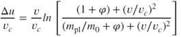
When ![]() the actual value for the jointly optimized payload ratio can be shown to be 0.46, with corresponding ratios of vehicle velocity increment as 0.299 and propellant exhaust velocity as 0.892. Further scrutiny indicates that this peak is rather broad and that payload ratios between 0.34 and 0.58 are within 6% of the mathematical optimum. Since engine parameters are rather “inelastic,” and since spacecraft designers deal with numerous constraints that are not propulsion related, using this wider range of optima is a practical necessity.
the actual value for the jointly optimized payload ratio can be shown to be 0.46, with corresponding ratios of vehicle velocity increment as 0.299 and propellant exhaust velocity as 0.892. Further scrutiny indicates that this peak is rather broad and that payload ratios between 0.34 and 0.58 are within 6% of the mathematical optimum. Since engine parameters are rather “inelastic,” and since spacecraft designers deal with numerous constraints that are not propulsion related, using this wider range of optima is a practical necessity.
Given the desirable 0.34 to 0.58 optimum payload‐ratio range, under this method of optimization we may select one or more thrusters within the range ![]() , where the optimized specific impulse
, where the optimized specific impulse ![]() is in seconds and the velocity change in m/sec. Since the vehicle's change in velocity is known, this criterion yields the resulting desirable limits in specific impulse. Figure 17–13 shows curves depicting the parameters in Eq. 17–38 for
is in seconds and the velocity change in m/sec. Since the vehicle's change in velocity is known, this criterion yields the resulting desirable limits in specific impulse. Figure 17–13 shows curves depicting the parameters in Eq. 17–38 for ![]() in an expanded dual‐optimum neighborhood. The oval insert encloses an expanded region of interest, one bounded by a contour curve, which represents values 10% below the mathematical peak.
in an expanded dual‐optimum neighborhood. The oval insert encloses an expanded region of interest, one bounded by a contour curve, which represents values 10% below the mathematical peak.

Figure 17–13 Payload fractions in the neighborhood of the dual optimum. The oval represents a contour 10% below the dual‐optimum peak. The parameters  and
and  in Fig. 17–3 are shown here in their equivalent form.
The utility of this approach hinges on the validity of the employed engine information. In particular, the specific power should represent all the inert components of the propulsion system that can be identified to depend on the power level. Payload mass must reflect all the mass that is neither proportional to the electrical power nor propellant related in addition to the actual “payload.” The tankage fraction must be proportional to the total propellant mass as required for Eq. 17–38. It has been assumed that there is available a source of electricity (typically from 28 to 300 VDC for solar‐powered craft) which is not tagged to the propulsion system. Our analysis also assumes that the efficiency is not a function of specific impulse (in contrast to Ref. 17–29); this implies the use an average or effective efficiency value at the relevant specific impulses. Since each individual thruster inside the oval of Fig. 17–13 only spans a limited range of specific impulse, this assumption is not too restrictive. During the continuous thrust schedules required by electric propulsion systems, thrust time represents mission time.
17.5 MISSION APPLICATIONS
Three principal application areas have been mentioned at the introduction to this chapter. The selection of a particular electric propulsion system for any given flight application depends not only on the characteristics of the propulsion system but also on the propulsive requirements of the particular flight mission and on the proven performance of the specific candidate propulsion system along with vehicle interfaces and the power conversion and storage systems. In general, the following criteria can be enumerated:
- For very precise low‐thrust station‐keeping and attitude control applications, pulsed thrusters are best suited. Some systems, however, utilize continuous thrust because pulsing generates noise or vibrations that cannot be tolerated.
- For deep‐space missions where the vehicle velocity increment is substantial, systems with very high specific impulse will give better performance. This is seen from the ratio
 at the dual optimum location (data from Fig.17–13).
 - While very high spacecraft velocity increments optimize at the higher specific impulses, propulsive times also increase and more rapidly (as shown in Section 17.1, the optimum specific impulse is nearly proportional to the square root of the thrust operating time, from
 and Eq. 17–8). This makes the optimum thrust and corresponding power generally lower which is favorable to electrostatic and electromagnetic units that operate exclusively in the specific impulse range above 1000 sec. See Example 17–4.
 - Since most missions of interest require long life, system reliability is a key selection criterion. Extensive testing under all likely environmental conditions (temperatures, accelerations, vibration, and radiation) under zero pressure and zero‐gravity is required for high reliability. Ground testing and qualification of electric engines needs to be as thorough as that of their chemical counterparts. Earth bound simulation of the low pressures in space requires large vacuum test chambers.
- There is a premium gain for high thruster efficiencies and high power‐conversion efficiencies. These will reduce the propellant mass, the inert mass of the power supply system and reduce thermal control requirements, all of which translate into lower total mass and higher vehicle performance. Technology advances in specific power (
 ) and decreases in tankage fraction (
 ) are also desirable toward minimizing inert mass.
 - For every propulsion mission there is a theoretically optimum range of specific impulse (see Fig. 17–3) and thus an optimum electrical propulsion scheme. While this optimum could be superseded by other conflicting system constraints (e.g., flight time or maximum power or size constraints or cost), the present inventory of proven electrical propulsion systems should meet most goals after some modifications.
- The present state of the art in electrical power sources may limit the type and size of electric propulsion systems that can be used for missions to the outer planets, unless nuclear energy power generation on board the spacecraft is further developed and its launch safety concerns become more acceptable to society.
- Practical factors, such as the storing and feeding of liquids in zero gravity, the availability of propellant (in the case of xenon), the conditioning of power to the desired voltage, frequency, and pulse duration, as well as redundancies in key system elements, the survival of sensors or controllers in long flights, and the inclusion of automatic self‐checking devices along with cost, all influence the selection and application of specific types of electric propulsion rockets.
- In addition to tankage and other internal considerations, propellant selection will also be governed by certain interface criteria such as plume noninterference with communication signals. Plumes must also be thermally benign and noncondensing on sensitive surfaces of the spacecraft such as optical windows, mirrors, and solar cells. See Chapter 20.
- Selection methods may evolve as one or more flight‐proven electrical propulsion systems become available. Also, it may be possible and more practical to modify a less than optimum existing proven unit to meet a desired new application.
Synchronous or geostationary satellites are of particular interest for communications and earth observation; their long life requires extensive station‐keeping propulsion requirements. Until recently, the main limitation to any such life increase had been the propellant mass requirement. There are also electric propulsion opportunities for orbit raising from LEO to GEO and there is interest in including propulsion system that can do both orbit rising and station keeping. “All‐Electric” is a recently minted term that refers to satellites that do not use conventional chemical propellants to reach their operational orbit; although such orbit‐raising process may take somewhat longer, the satellites themselves are much lighter than those with chemical propellant of similar means and they retain the capability to change orbital planes after launch. Earth satellites in inclined orbits with precise time–trajectory position requirements need propulsion units to maintain such orbits for counteracting certain perturbing natural forces, as described in Chapter 4. Drag compensation in low earth orbit (atmospheric skimming) satellites can be accomplished with electric thrusters.
Increasing life trends in earth‐orbit satellites from a minimum of 8 years to at least 15 years significantly increases their total impulse and the durability requirements of their propulsion system. For example, the north–south station‐keeping (NSSK) function of a typical geosynchronous satellite requires about 40,000 to 45,000 N‐sec or 9000 to 10,000 lbf‐sec of impulse per year. Table 17–8 shows some of the characteristics required of small and large electric thrusters for various propulsion functions in space. A good review of the state of the art up to 1997 is found in Ref. 17–30.
Table 17–8 Space Propulsion Application and Characteristics for Three Thrust Levels of Electric Propulsion Thrustersa
| Thrust Class | Application (Life) | Characteristics | Status |
| Micronewtons ( |
E–W station keeping Attitude control Momentum wheel unloading (15–20 years) Formation Flyingb |
10–500 W power Precise impulse bits of ∼ 2 × 10⁻⁵ N‐sec |
Operational & in development (micropropulsion) |
| Millinewtons (mN) |
N–S station keeping Orbit changes Drag cancellation Vector positioning (20 years) |
Kilowatts of power Impulse bits < 2 × 10⁻³ N‐sec for N–S, impulse/year of 46,000 N‐sec/100 kg spacecraft mass |
Operational |
| 0.01–10 N |
Orbit raising Interplanetary travel Solar system exploration (1–5 years) |
Long duration 1 kW–300 kW of power Intermittent and continuous operation |
Operational |
a Presently, nearly 95% of mission's applications of electric propulsion are for auxiliary propulsion such as orbit maintenance.
b Formation Flying is used in several communication LEO satellites. By having exactly equal spans between, they can provide continuous coverage in the region under them.
17.6 ELECTRIC SPACE‐POWER SUPPLIES AND POWER‐CONDITIONING SYSTEMS
The availability of substantial amounts of electrical power in space is considered to be a key requirement for high thrust electrical propulsion. Several combinations of energy sources and conversion methods have reached prototype stages, but only solar cells (photovoltaic), isotope thermoelectric generation units (nuclear), and fuel cells (chemical) have advanced to the point of routine space flight operation. Power output capacity of larger operational systems has been increasing from the low one‐kilowatt range to the medium tens of kilowatts required for some missions. The high end of a hundred or more kilowatts is still pending some technological (and political) breakthroughs.
Space power level requirements have increased with the increased capacity of earth‐orbit communications satellites and with planned missions, both manned and robotic, to moons and nearby planets. Payload requirements and thrust duration dictate power levels. Commercial communications system power satellites can temporarily reduce their communications volume during orbit maintenance so that electric power supplies do not need a dedicated unit for the propulsion system, but larger power demands may need enhanced solar cell capabilities. Many communications satellites actually share part or all of the power‐conditioning equipment with their electric thrusters.
Power Generation Units
Electric power generation units are classified as either direct (no moving mechanical parts) or dynamic. When the primary driver is reliability and the total power is small, direct conversion has been preferred but, at the advent of the Space Shuttle era and with the manned International Space Station (ISS), dynamic systems are being reconsidered. Many diverse concepts have been evaluated for meeting the electrical power demands of spacecraft, including their electric propulsion needs. Direct energy conversion methods considered include photovoltaic, thermoelectric, thermionic, and electrochemical, while methods with moving parts include the Brayton, Rankine, and Stirling cycles.
Batteries
Batteries may basically be classified as either primary or secondary. Primary batteries consume their active materials and convert chemical energy into electrical. Secondary batteries store electricity by utilizing a reversible chemical reaction and are designed to be recharged many times. There are both dry‐cell and wet‐cell primary batteries. The importance of primary batteries passed with the short‐lived satellites of the early 1960s. Secondary batteries with recharging provisions afford electrical power at higher output levels and longer lifetimes than primary batteries. All batteries must be sealed against the space vacuum or housed inside pressurized compartments. Secondary batteries are a critical component of solar cell systems for power augmentation and emergency backup and for periods when the satellite is in the earth's shadow. Lithium‐ion batteries have been used in space applications since 2003 because they offer higher energy/power density and operating voltage than conventional ones.
Fuel Cells
Chemical fuel cells are conversion devices used to supply space‐power needs for two to four weeks and for power levels up to 40 kW in manned missions. A catalyzer controls the chemical reaction to yield electricity directly; there is also some heat evolved which must be removed to maintain a desirable fuel cell temperature. Fuel cells are too massive for both robotic and long‐duration missions, having also had some reliability problems, but technological improvements have considerably advanced their performance and attractiveness.
Solar Cell Arrays
Solar cells rely on the photovoltaic effect to convert the sun's electromagnetic radiation into electricity. In silicon cells, sunlight generates a voltage and a photocurrent across a p‐n junction running as an inverse photodiode. Commercially available devices have reached 20% efficiency, but single‐bandgap (i.e., single‐junction) semiconductors are restricted by a theoretical upper limit of 33.7%. Newer multijunction solar cells can circumvent this efficiency limit because each layer is made to absorb a separate part of the spectrum as the light passes though the stack; presently, arrays with greater than 24% efficiencies are in earth orbit with multijunction semiconductors (up to 46% laboratory efficiencies have been reported by Fraunhofer ISE/Soltec). Another aspect of typical solar cell arrays is that many had been originally designed for only a 28 VDC output, although the present designs such as those for the ISS bus operate at 160 VDC and the NSTAR/DAWN missions uses 80 to 160 VDC. Today, there are designs (termed high‐voltage or direct drives, Ref. 17–31) that output increased voltages from their solar cell arrays, up to 300 VDC and beyond. As they become more operational, their higher voltages will considerably simplify power‐conditioning equipment in many existing electric‐propulsion systems and that may result in valuable inert mass savings. But care must be taken to avoid electrostatic discharges that can more easily occur at some earth orbits.
Solar cells have supplied electrical power in most of long‐duration space missions. The first solar‐cell unit was launched in March 1958 on Vanguard I and successfully energized data transmission for six years. Solar arrays exist in sizes up to 10 kW and could grow to 10 MW sizes in earth orbits. Typically, solar cell arrays are designed with a 20% overcapacity to allow for material degradation toward “end of life.” Losses in performance are due to radiation and particle impact damage, particularly in the radiation belts around the Earth. There have been continuous improvements in cell efficiency, reliability, and power per unit mass; for example, standard silicon cells deliver 180 W/m2 with arrays of 40 W/kg. Newer gallium arsenide cells produce 220 W/m2 and are more radiation resistant than silicon cells; these cell arrays are presently space qualified and together with parabolic concentrators can reach 100 W/kg (Ref. 17–27).
Factors that affect the specific mass of a solar array, besides its conversion efficiency, include the solar constant (which varies inversely as the square of the distance from the sun) and the manufactured thinness of the cell. Orientation to the sun is a more critical factor when solar concentrators are being used. Cell output is a function of cell temperature; performance in present designs can drop as much as 20% for a 100 °F increase in operating temperature so that thermal control has been critical. Solar cell panel configurations can be (1) fixed and body mounted to the spacecraft, (2) rigid and deployable (protected during launch and positioned in space), (3) flexible panels that are deployed (rolled out or unfolded), and (4) deployable with solar concentrator capabilities.
In addition to the solar arrays, their structure, deployment, and orientation equipment, other required items that include batteries, power‐conditioning and distribution systems, must be assigned to the power source mass and volume. Despite their apparent bulkiness and battery dependence, solar‐cell electrical systems have emerged as the dominant generating‐power system for unmanned spacecraft.
Nuclear Thermoelectric and Thermionic Systems
Nuclear energy from long‐decay radioisotopes and in some cases from fission reactors has played some role in the production of electricity in space. Both thermoelectric (based on the Seebeck effect) and thermionic (based on the Edison effect) devices have been investigated. These generators have no moving parts and can be made of materials reasonably resistant to radioactive environments. But their specific power is relatively low and cost, availability, and efficiency have been a limiting factor. The Voyager 2 spacecraft has been powered by three radioisotope thermoelectric generators which collectively delivered 420 watts at launch (in 1977); this spacecraft has been in operation for 37 years (as of 2014).
Throughout the 1950s and 1960s nuclear fission reactors were regarded as the most promising way to meet the high power demands of space missions, particularly trips to the outer planets involving months and perhaps years of travel. Radioisotope thermoelectric power has been embodied in a series of SNAP (Systems for Nuclear Auxiliary Power) electrical generating units that were designed and tested, ranging from 50 W to 300 kW of electrical output. More recent space nuclear reactor programs include NASA's Project Prometheus and the Russian TOPAZ that has been space tested up to nearly 6 kW. The latter consists of sets of nuclear rods each surrounded by a thermionic generator. Usage of direct‐conversion nuclear power generation, like in NASA's Multi‐Mission Radioisotope Thermoelectric Generator (MMRTG), include powering the Mars Science Laboratory (Curiosity) currently exploring the planet.
Thermionic converters have a significant mass advantage over thermoelectric ones, based on their higher effective radiator temperatures. Since thermal efficiencies for both thermoelectric and thermionic conversion have been below 10% and since all unconverted heat must be radiated, at higher operating temperatures thermionic radiators can be less massive. Moreover, cooling must be present at times when no electricity is generated since the heat source cannot be “turned off.” Depending on the location of the waste heat, designs involving heat pipes or recirculating cooling fluids are needed.
Long‐Duration High‐Output Dynamic Systems
On earth, designs of electric power generation with outputs of 10 to 1000 kW have been based on Stirling or Rankine heat engine cycles with nuclear, chemical, and even solar power sources. Overall efficiencies can be between 10 and 40%, but the associated hardware remains complex, including bearings, pumps, reactors, control rods, shielding, compressors, turbines, valves, and heat exchangers. Superconducting magnets together with advances in the state‐of‐the‐art of seals, bearings, and flywheel energy storage have made some dynamic units relatively more attractive. There remain development issues about high‐temperature materials that will withstand intense nuclear radiation fluxes over several years and there are still some concerns about achieving the required reliability in such complex systems in the space environment. While limited small‐scale experiments have been conducted, the development of these systems remains a challenge. An advanced Stirling radioisotope generator (labeled Radioisotope Electric Propulsion, see Fig. 17–1) is under development to replace radioisotope thermoelectric generators (RTGs) for future NASA missions.
Power‐Conditioning Equipment (PCU or PPU)
Power‐conditioning units or equipment are a necessary component of electric propulsion systems because of inevitable mismatches in voltage, frequency, power rate, and other electrical properties between the space‐power generating unit and the electric thruster. Power‐conditioning equipment has been more expensive, more massive, and more difficult to qualify than the thruster itself. If the thrust is pulsed, as in the PPT, the power‐conditioning unit has to provide pulse‐forming networks for momentary high currents, exact timing of different outputs, and control and recharging of condensers. Electrostatic engines commonly require up to 1800 VDC (except for FEEPs); the output of solar‐cell arrays is typically 28 to 300 VDC, so there is a need for DC‐to‐DC inverters and step‐up transformers to accomplish this task. Often this equipment is housed in a single “black box,” termed the power conditioner. Modern conditioning equipment contains all the internal logic required to start, safely operate, and stop the thruster; it is controlled by on–off commands sent by the spacecraft control processor. Besides the above functions that are specific to each engine, power‐conditioning equipment may have to provide circuit protection and propellant flow control as well as necessary redundancies.
As may be apparent from Table 17–7, one of the largest contributors to the specific mass (![]() ) of any electric‐propulsion system can be the power‐conditioning equipment. Here, electrothermal units have the simplest and lightest conditioning equipment, some needing none. Ion engines, on the other hand, have the heaviest equipment, with Hall thrusters somewhere in between (Ref. 17–24). PPTs have tended to have a large mass, but advances in energy storage capacitors have improved this situation. In fact, advances in solid‐state electronic pulse circuits together with lighter, more efficient, and higher temperature power‐conditioning hardware are areas of great interest in electric propulsion. Equipment efficiency tends to be high, about 90% or more, but here heat is generated at low temperatures and must be radiated to maintain their required moderately low temperatures of operation. While most present electric propulsion systems share the spacecraft electrical “bus system,” in some applications where EPS acts as the primary propulsion a special electrical bus called a “Direct Drive” (Ref. 17–31) is provided. When feasible, direct drives may allow simplification or elimination of some conditioning equipment, but a low‐pass filter is still needed for electromagnetic interference (EMI) control (more information in Ref. 17–29).
) of any electric‐propulsion system can be the power‐conditioning equipment. Here, electrothermal units have the simplest and lightest conditioning equipment, some needing none. Ion engines, on the other hand, have the heaviest equipment, with Hall thrusters somewhere in between (Ref. 17–24). PPTs have tended to have a large mass, but advances in energy storage capacitors have improved this situation. In fact, advances in solid‐state electronic pulse circuits together with lighter, more efficient, and higher temperature power‐conditioning hardware are areas of great interest in electric propulsion. Equipment efficiency tends to be high, about 90% or more, but here heat is generated at low temperatures and must be radiated to maintain their required moderately low temperatures of operation. While most present electric propulsion systems share the spacecraft electrical “bus system,” in some applications where EPS acts as the primary propulsion a special electrical bus called a “Direct Drive” (Ref. 17–31) is provided. When feasible, direct drives may allow simplification or elimination of some conditioning equipment, but a low‐pass filter is still needed for electromagnetic interference (EMI) control (more information in Ref. 17–29).
SYMBOLS
| acceleration, m/sec2(ft/sec2) | |
| area, cm2 or m2 | |
| magnetic flux density, web/m2 or tesla | |
| radial magnetic flux density, web/m2 or tesla | |
| effective exhaust velocity, m/sec | |
| circuit capacitance, farad/m | |
| specific heat, J/kg‐K | |
| accelerator grid spacing, cm (in.) | |
| hole or beam diameter, cm (in.) | |
| electronic charge, 1.602 × 10⁻¹⁹ coulomb | |
| electric field, V/m | |
| longitudinal electric field, V/m | |
| transverse electric field, V/m | |
| microscopic force on a particle | |
| thrust force, N or mN (lbf or mlbf) | |
| accelerating force density inside channel, N/m3(lbf/ft3), see Eq. 17–14 | |
| constant converting propellant ejection velocity units to sec, 9.81 m/sec2 or 32.2 ft/sec2 | |
| total current, A | |
| impulse bit, N‐sec or lbf‐sec | |
| specific impulse, sec [ |
|
| current density, A/m2 | |
| orthogonal current density components | |
| Hall current density, A/m2 | |
| specific heat ratio | |
| ionization loss, W | |
| circuit inductance, henry | |
| propellant mass, kg (lbm) | |
| power plant mass, kg (lbm) | |
| payload mass, kg (lbm) | |
| initial total vehicle mass, kg (lbm) | |
| mass flow rate, kg/sec (lbm/sec) | |
| atomic or molecular mass, kg/kg‐mol (lbm/lb‐mol) | |
| electron number density, m−3(ft−3) | |
| number of pulses | |
| power, W | |
| electrical power, W | |
| kinetic power of jet, W | |
| inner radius, m | |
| outer radius, m | |
| plasma resistance, ohms | |
| distance, cm (in.) | |
| time or duration, sec | |
| propulsive time, sec [ |
|
| absolute temperature, K (°R) | |
| vehicle velocity change, m/sec (ft/sec) | |
| propellant or charged particle exhaust velocity, m/sec (ft/sec) | |
| plasma velocity or injection velocity along accelerator, m/sec | |
| characteristic speed, m/sec | |
| voltage, V | |
| Local or total accelerator voltage, V | |
| rail width, m | |
| linear dimension, m (ft) |
Greek Letters
| specific power, W/kg (W/lbm) | |
| electron Hall parameter (dimensionless) | |
| permittivity of free space, 8.85 × 10⁻¹² farad/m | |
| ionization potential, eV | |
| Hall thruster β‐efficiency | |
| thruster efficiency | |
| ion‐ratio of injected to gained accelerator energy ≥ 0 | |
| ion mass, kg | |
| electron mass, 9.11 × 10⁻³¹ kg | |
| permeability of free space, 4π × 10−7 henry/m | |
| tankage mass fraction | |
| space–charge, coulomb/m3 | |
| plasma electrical conductivity, mho/m | |
| mean collision time, sec (also characteristic time, sec) | |
| electron cyclotron frequency, (sec)−1 |
PROBLEMS
- The characteristic velocity
 is used to achieve a dimensionless representation of flight performance analysis. Derive Eq. 17–38 without any tankage fraction allowance (i.e.,
  ). Also, plot the payload fraction against
  for several values of
  . Discuss your results with respect to the optimum performance.
 - For the special case of zero payload in Problem 1, determine the maximized values of
 ,
,  ,
,  , and
, and  in terms of this characteristic velocity.Answer:
  ,
,  ,
,  ,
,  .
. - For a space mission with an incremental vehicle velocity of 85,000 ft/sec and a specific power of
 , determine the optimum values of
  and
and  for two maximum payload fractions, namely 0.35 and 0.55. Take the thruster efficiency as 100% and
  .Answer: For 0.35: Is = 5.11 × 10³ sec; tp = 2.06 × 10⁷ sec; for 0.55: Is = 8.88 × 10³ sec; tp = 5.08 × 10⁷ sec.
 - Derive Eq. 17–7 using
 instead of Eq. 17–6 (take
  ); this form penalizes the high
  and/or short
  missions. Plot and compare to the results shown on Fig. 17–3.
 - An ion thruster uses heavy positively charged particles with a charge‐to‐mass ratio of 500 coulombs per kilogram, producing a specific impulse of 3000 sec. (a) What two‐screen grid acceleration voltage would be required for this specific impulse? (b) If the accelerator spacing is 6 mm, what would be the diameter of an ion beam producing 0.5 N of thrust at this accelerator voltage?Answer: (a) 8.66 × 10⁵ V; (b) D = 1.97 mm.
- An argon ion thruster has the following characteristics and operating conditions:
- Voltage across ionizer = 400 V Voltage across accelerator = 3 × 10⁴ V
- Diameter of ion source = 5 cm Accelerator electrode spacing = 1.2 cm
 .
. - For a given power source of 300 kW electrical output, a propellant mass of 6000 lbm,
 , and a payload of 4000 lbm, determine the thrust, ideal velocity increment, and duration of powered flight for the following three cases:
- Arcjet:


- Ion engine:


- Hall engine:


 .
. .
. .
.
- Arcjet:
- A formulation for the exit velocity in an MPD that allows for a simple estimate of the accelerator length is shown below; these equations relate the accelerator distance to the velocity implicitly through the acceleration time
 . Considering a flow at a constant plasma of density
  (which does not choke), solve Newton's second law first for the speed
  and then for the distance
  and show that
where
and show that
where
 and has units of seconds. For this simplified plasma model of an MPD accelerator, calculate the distance needed to accelerate the plasma from rest up to
  and the time involved. Take the plasma conductivity as
  ,
,  ),
),  , and
, and  .Answer: 503 m, 0.1005 sec.
 - Assume that a materials breakthrough makes it possible to increase the operating temperature in the plenum chamber of an electrothermal engine from 3000 to 4000 K. Nitrogen gas is the propellant which is available from tanks at 250 K. Neglecting dissociation, and taking
 and
and  , calculate the old and new
  corresponding to the two temperatures. Operating or thrust time is 10 days, payload mass is 1000 kg, and k = 1.3 for the hot diatomic molecule.Answer: 610 m/sec old, 711 new.
 - An arcjet delivers 0.26 N of thrust. Calculate the vehicle velocity increase under gravitationless, dragless flight for a 28‐day thrust duration with a payload mass of 100 kg. Take thruster efficiency as 50%, specific impulse as 2600 sec, and specific power as 200 W/kg. This is not an optimum payload fraction; estimate an
 which would maximize the payload fraction with all other factors remaining the same.Answer:
  ;
;  (decrease).
 - A patent application describes an electrostatic thruster that accelerates electrons as the propellant. The inventor points out that the space–charge limited thrust is independent of the propellant mass and that electrons are very easy to produce (by cathode surface emission) and much easier to accelerate than atomic ions. Show using the basic relationships for electrostatic thrusters given in this chapter that electron acceleration is impractical for electrostatic thrusters. Assume that the required thrust is 10− 5 N per accelerator hole, that there are several thousand holes of “aspect ratio”
 in the accelerator, and that the neutralizer operates with protons (which have a mass 1836 times that of the electron).
 - For each of the three thrusters in Example 17–4, calculate the thrust F and input power Pe that would apply for a payload mass
 of 100 kg. What would result if the spacecraft power supply is limited to 30 kW but mission time could extend up to 100 days?Answer: Arcjet: 0.754 N, 9.24 kW; Hall: 1.73 N, 29.6 kW; Ion: 1.49 N, 40.9 kW.
REFERENCES
- 17–1. M. M. Micci and A. D. Ketsdever (Eds.), Micropropulsion for Small Spacecraft, Progress in Astronautics and Aeronautics, Vol. 187, AIAA, Reston, VA, 2000; J. Mueller et al., “Survey of Propulsion options for Cubesats,” Jet Propulsion Laboratory Caltech, CPIAC JSD CD‐62 (Abstract No. 2010‐9915BP).
- 17–2. R. G. Jahn, Physics of Electric Propulsion, McGraw‐Hill Book Company, New York, 1968, pp. 103–110. See also http://alfven.princeton.edu/papers/Encyclopedia.pdf
- 17–3. D. M. Goebel and I. Katz, Fundamentals of Electric Propulsion—Ion and Hall Thrusters, John Wiley and Sons, Hoboken, NJ, 2008.
- 17–4. P. J. Turchi, Chapter 9, “Electric Rocket Propulsion Systems,” in R. W. Humble, G. N. Henry, and W. J. Larson (Eds.), Space Propulsion Analysis and Design, McGraw‐Hill, New York, 1995, pp. 509–598.
- 17–5. A. Spitzer, “Near Optimal Transfer Orbit Trajectory Using Electric Propulsion,” AAS Paper 95–215, American Astronautical Society Meeting, Albuquerque, NM, Feb. 13–16, 1995.
- 17–6. D. B. Langmuir, Chapter 9, “Low‐Thrust Flight: Constant Exhaust Velocity in Field‐Free Space,” in H. Seifert (Ed.), Space Technology, John Wiley & Sons, New York, 1959.
- 17–7. D. C. Byers and J. W. Dankanich, “Geosynchronous Earth Orbit Communication Satellite Deliveries with Integrated Electrical Propulsion,” Journal of Propulsion and Power, Vol. 24, No. 6, 2008, pp. 1369–1375.
- 17–8. M. J. Patterson, L. Pinero, and J. S. Sovey, “Near‐Term High Power Ion Propulsion Options for Earth‐Orbital Applications,” AIAA Paper 2009–4819, Denver, Colorado, Aug. 2009.
- 17–9. F. R. Chang Diaz, et al, VASIMR Engine: Project Status and Recent Accomplishments, AIAA Paper 2004‐0149, Reno Nevada, Jan. 2004; see also Wikipedia entry: Variable Specific Impulse Magnetoplasma Rocket.
- 17–10. C. D. Brown, Spacecraft Propulsion, AIAA Education Series, Washington, DC, 1996.
- 17–11. F. F. Chen, Introduction to Plasma Physics, Plenum Press, New York, 1974.
- 17–12. G. W. Sutton and A. Sherman, Engineering Magnetohydrodynamics, McGraw‐Hill Book Company, New York, 1965.
- 17–13. D. M. Zube et al., “History and Recent Developments of Aerojet Rocketdyne's MR‐510 Hydrazine Arcjet Systems,” Space Propulsion Conference 2014, paper SP2014_2966753, Cologne, Germany.
- 17–14. D. R. Bromaghim et al., “Review of the Electric Propulsion Space Experiment (ESEX) Program,” Journal of Propulsion and Power, Vol. 18, No. 4, July–August 2002, pp. 723–730.
- 17–15. J. Mueller, Chapter 3, in Ref. 17–1.
- 17–16. M. Tajmar, A. Genovese, and W. Steiger, “Indium Field Emission Electric Propulsion Microthruster Experimental Characterization,” Journal of Propulsion and Power, Vol. 20, No. 2, Mar.–Apr. 2004.
- 17–17. J. R. Beattie, XIPS Keeps Satellites on Track, The Industrial Physicist, Vol. 4, No. 2, Jun. 1998; C. E. Garner and M. D. Rayman, “In Flight Operation of the Dawn Ion Propulsion System Through Survey Science Orbit at Ceres,” paper AIAA 2015‐3717, Orlando, FL, 2015.
- 17–18. K. J. Groh and H. W. Loeb, State of the Art of Radio Frequency Ion Thrusters, J. Propulsion, Vol. 7 No. 4, Jul.–Aug. 1991, pp. 573–579; N. Nishiyama et al., “In‐Flight Operation of the Haybusa2 Ion Engine System in the EDVEGA Phase,” paper AIAA 2015‐3718, Orlando, FL, 2015.
- 17–19. P. G. Hill and C. R. Peterson, Mechanics and Thermodynamics of Propulsion, Addison‐Wesley Publishing Company, Reading, MA, 1992.
- 17–20. S. Liu and R. A. Dougal, “Initial Velocity Effect on Space‐Charge‐Limited Currents,” Journal of Applied Physics, Vol. 78, No. 10, Nov. 16, 1995, pp. 5919–59–25; O. Biblarz, “Ion Accelerator Currents Beyond the Child‐Langmuir Limit,” AIAA Paper 2013–4109, San Jose, CA, Jul. 2013.
- 17–21. E. L. Resler, Jr., and W. R. Sears, “Prospects of Magneto‐Aerodynamics,” Journal of Aeronautical Sciences, Vol. 24, No. 4, Apr. 1958, pp. 235–246.
- 17–22. S. S. Bushman and R. L. Burton, “Heating and Plasma Properties in a Coaxial Gasdynamic Pulsed Plasma Thruster,” Journal of Propulsion and Power, Vol. 17, No. 5, Sept.–Oct. 2001, pp. 959–966.
- 17–23. V. Kim, “Main Physical Features and Processes Determining the Performance of Stationary Plasma Thrusters,” Journal of Propulsion and Power, Vol. 14, No. 5, Sept.–Oct. 1998, pp. 736–743.
- 17–24. C. H. McLean, J. B. McVey, and D. T. Schappell, “Testing of a U.S.‐Built HET System for Orbit Transfer Applications,” AIAA Paper 99‐2574, Jun. 1999.
- 17–25. B. Welander et al., “Life and Operating Range Extension of the BPT 4000 Qualification Model Hall Thruster,” AIAA Paper 2006–5263, Sacramento, CA, Jul. 2006.
- 17–26. D. Baker, Chapter 10, “Mission Design Case Study,” in R. W. Humble, G. N. Henry, and W. J. Larson (Eds.), Space Propulsion Analysis and Design, McGraw‐Hill, New York, 1995.
- 17–27. M. Martinez‐Sanchez and J. E. Pollard, “Spacecraft Electric Propulsion—An Overview,” Journal of Propulsion and Power, Vol. 14, No. 5, Sept.–Oct. 1998, pp. 688–699.
- 17–28. J. D. Filliben, “Electric Propulsion for Spacecraft Applications,” Chemical Propulsion Information Agency Report CPTR 96‐64, The Johns Hopkins University, Dec. 1996.
- 17–29. M. A. Kurtz, H. L. Kurtz, and H. O. Schrade, “Optimization of Electric Propulsion Systems Considering Specific Power as a Function of Specific Impulse,” Journal of Propulsion and Power, Vol. 4, No. 2, 1988, pp. 512–519.
- 17–30. J. D. Filliben, “Electric Thruster Systems,” Chemical Propulsion Information Agency Report CPTR‐97‐65, The Johns Hopkins University, Jun. 1997.
- 17–31. T. W. Kerslake, “Effect of Voltage Level on Power System Design for Solar Electric Propulsion Missions,” Journal of Solar Energy Engineering, Vol. 126, No. 3, Aug. 2004, pp. 936–944.