
CHAPTER 4
FLIGHT PERFORMANCE
This chapter serves as an introduction to the flight performance of rocket‐propelled vehicles such as spacecraft, space launch vehicles, and missiles or projectiles. It presents these subjects from a rocket propulsion point of view. Propulsion systems deliver forces to a flight vehicle and cause it to accelerate (or at times decelerate), overcome drag forces, or to change flight direction. Some propulsion systems also provide torques to the flight vehicles for rotation or other maneuvers. Flight missions can be classified into several flight regimes: (1) flight within the Earth's atmosphere (e.g., air‐to‐surface missiles, surface‐to‐surface short‐range missiles, surface‐to‐air missiles, air‐to‐air missiles, assisted takeoff units, sounding rockets, or aircraft rocket propulsion systems), see Refs. 4–1 and 4–2; (2) near space environment (e.g., Earth satellites, orbital space stations, or long‐range ballistic missiles), see Refs. 4–3 to 4–9; (3) lunar and planetary flights (with or without landing or Earth return), see Refs. 4–5 to 4–12; and (4) deep space exploration and sun escape. Each of these is discussed in this chapter except for the operation of very low thrust units which is treated in Chapter 17. We begin with a basic one‐dimensional analysis of space flight and then consider some more the complex fight path scenarios for various flying rocket‐propelled vehicles. Conversion factors, atmospheric properties, and a summary of key equations can be found in the appendices.
4.1 GRAVITY‐FREE DRAG‐FREE SPACE FLIGHT
This simplified rocket flight analysis applies to outer space environments, far enough from any star, where there is no atmosphere (thus no drag) and essentially no significant gravitational attraction. The flight direction is the same as the thrust direction (along the axis of the nozzle, namely, a linear acceleration path); the propellant mass flow is ![]() and the propulsive thrust F remains constant for the propellant burning time duration tp. The thrust force F has been defined in Eq. 2–16. For constant propellant flow, the flow rate
and the propulsive thrust F remains constant for the propellant burning time duration tp. The thrust force F has been defined in Eq. 2–16. For constant propellant flow, the flow rate ![]() becomes mp/tp, where mp is the total usable propellant mass. From Newton's second law and for an instantaneous vehicle mass m with flight velocity u,
becomes mp/tp, where mp is the total usable propellant mass. From Newton's second law and for an instantaneous vehicle mass m with flight velocity u,
For any rocket where start and shutdown durations may be neglected, the instantaneous mass of the vehicle m may be expressed as a function of time t using the initial mass of the full vehicle m0, the initial propellant mass mp, the time at power cutoff tp as follows:
Equation 4–3 expresses the vehicle mass in a form useful for trajectory calculations. The total vehicle mass ratio ![]() and the propellant mass fraction ζ have been defined in Eqs. 2–7 and 2–8 (see section 4.7 for an extension to multistage vehicles). They are related by
and the propellant mass fraction ζ have been defined in Eqs. 2–7 and 2–8 (see section 4.7 for an extension to multistage vehicles). They are related by
A depiction of the relevant masses is shown in Fig. 4–1. The initial mass at takeoff m0 equals the sum of the useful propellant mass mp plus the empty or final vehicle mass mf; in turn mf equals the sum of the inert masses of the engine system (such as nozzles, tanks, cases, or unused residual propellant) plus the guidance, control, electronics, and related equipment and the payload. After thrust termination, any residual propellant in the propulsion system is considered to be a part of the final engine mass. This includes any liquid propellant remaining in tanks after operation, trapped in pipe pockets, valve cavities, and pumps or wetting the tank and pipe walls. For solid propellant rocket motors it is the remaining unburned solid propellant, also called “slivers,” and sometimes also unburned insulation.

Figure 4–1 Definitions of various vehicle masses. For solid propellant rocket motors the words “rocket engine, tanks, and structures” are to be replaced by “rocket motor nozzle, thermal insulation, and case.” mp includes only the usable propellant mass; residuals are part of the empty mass.
For constant propellant mass flow ![]() and finite propellant burning time tb the total useful propellant mass mp is simply
and finite propellant burning time tb the total useful propellant mass mp is simply ![]() and the instantaneous vehicle mass
and the instantaneous vehicle mass ![]() . Equation 4–1 may be written as
. Equation 4–1 may be written as

When start and shutdown periods consume relatively little propellant, they may be neglected. Integration leads to the maximum vehicle velocity up at propellant burnout that can be attained in a gravity‐free vacuum environment. Depending on the frame of reference, u0 will not necessarily be zero, and the result is often written as a velocity increment Δu:
However, when the initial velocity u0 may be taken as zero, the velocity at thrust termination up becomes

The symbol “ln” stands for the natural logarithm. Thus, up is the maximum velocity increment Δu that can be obtained in a gravity‐free vacuum with constant propellant flow, starting from rest. The effect of variations in c, Is, and ζ on this flight velocity increment is shown in Fig. 4–2. An alternate way to write Eq. 4–6 using “e,” the base of the natural logarithm is

Figure 4–2 Maximum vehicle flight velocity in gravitationless, drag‐free space for different mass ratios and specific impulses (plot of Eq. 4–6). Single‐stage vehicles can have values of  up to about 20 and multistage vehicles can exceed 200.
The concept of maximum attainable flight velocity increment Δu in a gravity‐free vacuum is valuable for understanding the influence of the basic parameters involved. It is used in comparing one propulsion system on a vehicle or one flight mission with another, as well as in comparing proposed upgrades or possible design improvements.
From Eq. 4–6 it can be seen that the vehicle's propellant mass fraction has a logarithmic effect on the vehicle velocity. By increasing this ratio from 0.80 to 0.90, up is increased by 43%. A mass fraction of 0.80 indicates that only 20% of the total vehicle mass is needed for structure, skin, payload, propulsion hardware, radios, guidance system, aerodynamic lifting surfaces, and so on; the remaining 80% is useful propellant. To exceed 0.85 requires a careful design; mass fraction ratios approaching 0.95 appear to be the probable practical upper limit for single‐stage vehicles with currently known materials (when the mass fraction is 0.90, then ![]() or
or ![]() ). This noticeable influence of mass fraction or mass ratio on the velocity at power cutoff, and therefore also on vehicle range, is fundamental and applies to most types of rocket‐powered vehicles. For this reason, high importance is placed on saving inert mass on each and every vehicle component, including the propulsion system.
). This noticeable influence of mass fraction or mass ratio on the velocity at power cutoff, and therefore also on vehicle range, is fundamental and applies to most types of rocket‐powered vehicles. For this reason, high importance is placed on saving inert mass on each and every vehicle component, including the propulsion system.
Equation 4–6 can be solved for the effective propellant mass mp required to achieve a desired velocity increment for a given initial takeoff mass or a final shutdown mass of the vehicle. The final mass consists of the payload, the structural mass of the vehicle, the empty propulsion system mass (that includes residual propellant), plus a small additional mass for guidance, communications, and control devices. Here ![]() :
:

Figure 4–3 Maximum payload fraction in gravitationless, drag‐free space, single‐stage vehicle flight for different stage‐mass fractions, velocity increments and specific impulses. For each stage  and Eq. 2–8 becomes
  .
.
In a gravity‐free environment, the flight velocity increment Δu or up is proportional to the effective exhaust velocity c and, therefore, to the specific impulse (see Eq. 2–6). Thus, any improvement in Is (such as better propellants, more favorable nozzle area ratios, or higher chamber pressures) reflects itself in improved vehicle performance, provided that such an improvement does not also necessitate an excessive increase in rocket propulsion system inert mass, which would lead to a decrease in the effective propellant fraction. Figure 4–3 shows how payload fraction (![]() ) varies as a function of the ratio (
) varies as a function of the ratio (![]() ) for several values of propellant stage‐mass fraction ζi, as calculated from the equations introduced above for single‐staged vehicles. Figure 4–3 complements Fig. 4–2 showing
) for several values of propellant stage‐mass fraction ζi, as calculated from the equations introduced above for single‐staged vehicles. Figure 4–3 complements Fig. 4–2 showing ![]() as a function of both
as a function of both ![]() and ζi (Example 4–3 treats ζi for multi‐staged vehicles). Note that for any given ζi < 1.0 certain payload fractions become unavailable as values of
and ζi (Example 4–3 treats ζi for multi‐staged vehicles). Note that for any given ζi < 1.0 certain payload fractions become unavailable as values of ![]() increase. This is evident for the three curves that terminate at zero payload fraction.
increase. This is evident for the three curves that terminate at zero payload fraction.
4.2 FORCES ACTING ON A VEHICLE IN THE ATMOSPHERE
The external forces commonly acting on vehicles flying in the Earth's atmosphere consist of thrust, aerodynamic forces, and gravitational attractions. Other forces, such as wind or solar radiation pressure, are usually small and generally can be neglected in many calculations.
Thrust is the force produced by the vehicle's power plant, such as a propeller or a rocket propulsion system. It most often acts in the direction of the axis of the power plant, that is, along the propeller shaft axis or the rocket nozzle axis. The thrust force of a rocket propulsion system with constant mass flow has been formulated in Chapter 2 as a function of the effective exhaust velocity c and the propellant flow rate ![]() . In many rockets the mass rate of propellant consumption
. In many rockets the mass rate of propellant consumption ![]() is essentially constant, and starting and stopping transients may be neglected. Therefore, the thrust as given from Eq. 2–6 (or Eqs. 2–13 and 2–15) may be written with
is essentially constant, and starting and stopping transients may be neglected. Therefore, the thrust as given from Eq. 2–6 (or Eqs. 2–13 and 2–15) may be written with ![]() as
as ![]()
As explained in Chapter 3, the value of the effective exhaust velocity c (or the specific impulse Is) depends on both nozzle area ratio and nozzle exhaust pressure. However, as Earth altitude increases, values of c change only by a relatively small factor bounded between about 1.2 and 1.8 (with the higher values applicable in the vacuum of space).

Figure 4–4 Variation of lift and drag coefficient with Mach number of the German V‐2 missile at several angles of attack α based on body cross‐sectional area with jet off and without exhaust plume effects. The Mach number shown, defined in Eq. 3–11, relates to the external flow.
There are two relevant aerodynamic forces in the atmosphere. The drag D acts in a direction opposite to the flight path and is due to resistance to the body's motion by the surrounding fluid. The lift L is the aerodynamic force acting in a direction normal to the flight path. They are both given as functions of the vehicle's flight speed u, the mass density ρ of the atmosphere in which it moves, and a characteristic surface area A:
where CL and CD are lift and drag coefficients, respectively. For airplanes and winged missiles the area A is the wing area. For wingless missiles or space launch vehicles it is the maximum cross‐sectional area normal to the missile axis. These lift and drag coefficients are primarily functions of the vehicle configuration, flight Mach number, and angle of attack—the angle between the vehicle axis (or the wing plane) and the flight direction. At low flight speeds, Mach number effects may be neglected, and the drag and lift coefficients are only functions of the angle of attack. A typical variation of the drag and lift coefficients for a supersonic missile is shown in Fig. 4–4. Values for these coefficients reach a maximum near a Mach number of unity. For wingless vehicles the effective angle of attack α is usually very small ![]() . The “standard density” and other properties of the Earth's atmosphere are listed in Appendix 2, but note that the local density can vary from day to day by a factor up to 2 (for altitudes from 300 to 1200 km) depending on solar activity and night‐to‐day temperature variations. This introduces a major uncertainty in calculations of lift and drag. Aerodynamic forces are also affected by the flow and the pressure distribution of the rocket exhaust gases, as explained in Chapter 20.
. The “standard density” and other properties of the Earth's atmosphere are listed in Appendix 2, but note that the local density can vary from day to day by a factor up to 2 (for altitudes from 300 to 1200 km) depending on solar activity and night‐to‐day temperature variations. This introduces a major uncertainty in calculations of lift and drag. Aerodynamic forces are also affected by the flow and the pressure distribution of the rocket exhaust gases, as explained in Chapter 20.
A vehicle's flight regime in the neighborhood of Mach 1 is called the transonic flight region. Here strong unsteady aerodynamic forces often develop (due to shock‐induced buffeting), which are noticeable in the steep rise and subsequent decrease of the coefficients as shown in Fig. 4–4. In some cases a vehicle's maximum load capabilities during transonic flight have been exceeded leading to structural failures.
For properly designed space launch vehicles and ballistic missiles the integrated drag losses, when expressed in terms of Δu, are typically 5 to 10% of the final ideal vehicle velocity. These relatively low values result from air densities (and thus dynamic pressures), being low at high altitudes where velocities are high, and being high at altitudes where vehicle velocities are low.
Gravitational attraction is exerted upon any flying space vehicle by all planets, stars, and moons. Gravity forces pull the vehicle in the direction of the center of mass of the attracting body. Within the immediate vicinity of the Earth, the attraction of other planets and celestial bodies (like our sun and moon) can be negligibly small compared to the Earth's gravitational force. This force or gravitational pull makes up the object's weight.
When Earth gravity variations with the geographical features and the oblate shape are neglected, the acceleration of gravity g varies inversely as the square of the distance from the Earth's center. If R0 is the mean radius at the (spherical) Earth's surface at which g0 is the acceleration of gravity, by Newton's law of gravitation, g changes with altitude (h) as

At the equator the spherical Earth's radius is ![]() and the standard value of g0 is 9.80665 m/sec2. At distances as far away as the moon, the Earth's gravity acceleration is only about
and the standard value of g0 is 9.80665 m/sec2. At distances as far away as the moon, the Earth's gravity acceleration is only about ![]() . For the most accurate analyses, the value of g will vary locally with the Earth's bulge at the equator, with the height of nearby mountains, and with the local difference of the Earth's density at specific regions.
. For the most accurate analyses, the value of g will vary locally with the Earth's bulge at the equator, with the height of nearby mountains, and with the local difference of the Earth's density at specific regions.
4.3 BASIC RELATIONS OF MOTION
For any vehicle that flies within the Earth's proximity, the gravitational attractions from all other heavenly bodies are neglected. Assume next that the vehicle is moving in rectilinear equilibrium flight and that all control forces, lateral forces, and moments that tend to turn the vehicle are zero. The resulting trajectory is two‐dimensional and is contained in a fixed plane. Assume further that the vehicle has wings inclined to the flight path at an angle of attack α providing lift in a direction normal to the flight path. The direction of flight need not coincide with the direction of thrust as shown schematically in Figure 4–5.

Figure 4–5 Two‐dimensional free‐body force diagram for flying vehicle with wings and fins.
Let θ be the angle of the flight path with the horizontal and ψ the angle of the direction of thrust with the horizontal. Along the flight path direction, the product of the mass and the acceleration has to equal the vector sum of the propulsive, aerodynamic, and gravitational forces:
The acceleration perpendicular to the flight path is ![]() ; for a given value of u and at the instantaneous Earth radius R (from the Earth's center) of the flight path, it becomes u2/R. The equation of motion in a direction normal to the flight velocity is
; for a given value of u and at the instantaneous Earth radius R (from the Earth's center) of the flight path, it becomes u2/R. The equation of motion in a direction normal to the flight velocity is
By substituting from Eqs. 4–10 and 4–11, these two basic equations can be solved for the accelerations as follows:
No general solution can be given to these equations, since ![]() , and/or ψ may vary independently with time, mission profile, and/or altitude. Also, CD and CL are functions of velocity or Mach number. In more sophisticated analyses, other factors may also be considered, such as any propellant used for nonpropulsive purposes (e.g., attitude control or flight stability). See Refs. 4–1, 4–8, 4–11, and 4–12 for background material on flight performance in some of these flight regimes. Because rocket propulsion systems are usually tailored to fit specific flight missions, different flight performance parameters are maximized (or optimized) for different rocket flight missions or flight regimes such as Δu, range, orbit height and shape, time‐to‐target, or altitude.
, and/or ψ may vary independently with time, mission profile, and/or altitude. Also, CD and CL are functions of velocity or Mach number. In more sophisticated analyses, other factors may also be considered, such as any propellant used for nonpropulsive purposes (e.g., attitude control or flight stability). See Refs. 4–1, 4–8, 4–11, and 4–12 for background material on flight performance in some of these flight regimes. Because rocket propulsion systems are usually tailored to fit specific flight missions, different flight performance parameters are maximized (or optimized) for different rocket flight missions or flight regimes such as Δu, range, orbit height and shape, time‐to‐target, or altitude.
For actual trajectory analyses, navigation computation, space flight path determination, or missile‐firing tables, the above two‐dimensional simplified theory is not sufficiently accurate; perturbation effects, such as those listed in Section 4.4, must then be considered in addition to drag and gravity, and computer modelling is necessary to handle such complex relations. Suitable divisions of the trajectory into small elements and step‐by‐step or numerical integrations to define a trajectory are usually indicated. More generally, three‐body theories include the gravitational attraction among three masses (for example, the Earth, the moon, and the space vehicle) and this is considered necessary in many space flight problems (see Refs. 4–2 to 4–5). The form and the solution to the given equations become further complicated when propellant flow and thrust are not constant and when the flight path is three dimensional.
For each mission or flight one can obtain actual histories of velocities and distances traveled and thus complete trajectories when integrating Eqs. 4–15 and 4–16. More general cases require six equations: three for translation along each of three perpendicular axes and three for rotation about these axes. The choice of coordinate systems of reference points can simplify the mathematical solutions (see Refs. 4–3 and 4–5) but there are always a number of trade‐offs in selecting the best trajectory for the flight of a rocket vehicle. For example, for a fixed thrust the trade‐off is between burn time, drag, payload, maximum velocity, and maximum altitude (or range). Reference 4–2 describes the trade‐offs between payload, maximum altitude, and flight stability for sounding rockets.
Equations 4–15 and 4–16 may be further simplified for various special applications, as shown below; results of such calculations for velocity, altitude, or range using the above two basic equations are often adequate for rough design estimates. A form of these equations is also useful for determining the actual thrust or actual specific impulse during vehicle flight from accurately observed trajectory data, such as from optical or radar tracking data. Vehicle acceleration (du/dt) is essentially proportional to net thrust and, by making assumptions or measurements of propellant flow (which usually varies in a predetermined manner) and from analyses of aerodynamic forces, it is possible to determine a rocket propulsion system's actual thrust under flight conditions.
Equations 4–15 and 4–16 simplify for wingless rocket projectiles, space launch vehicles, or missiles with constant thrust and propellant flow. In Fig. 4–6 the flight direction θ is the same as the thrust direction and any lift forces for a symmetrical, wingless, stably flying vehicle are neglected at zero angle of attack. For a two‐dimensional trajectory in a single plane (no wind forces) and a stationary Earth, the acceleration in the direction of flight is given below, where tp is the operating or burn time of the propellant and ![]() is the propellant mass fraction:
is the propellant mass fraction:
The force vector diagram in Fig. 4–6 also shows the net force (the addition of thrust, drag, and gravity vectors) to be at an angle to the flight path, which will therefore be curved. These types of diagram form the basis for iterative trajectory numerical solutions.

Figure 4–6 Simplified free‐body force diagram for a vehicle without wings or fins. The force vector diagram shows the net force on the vehicle. All forces act through the vehicle's center of gravity.
All further relationships in this section correspond to two‐dimensional flight paths, ones that lie in a single plane. If maneuvers out of that plane take place (e.g., due to solar attraction, thrust misalignment, or wind), then another set of equations will be needed—it requires both force and energy to push a vehicle out of its flight plane; Reference 4–1 describes equations for the motion of rocket projectiles in the atmosphere in three dimensions. Trajectories must be calculated accurately in order to reach any intended flight objective and today these are done exclusively with the aid of computers. Several computer programs for analyzing flight trajectories exist (which are maintained by aerospace companies and/or government agencies). Some are two‐dimensional, relatively simple, and used for making preliminary estimates or comparisons of alternative flight paths, alternative vehicle designs, or alternative propulsion schemes. Several use a stationary flat Earth, while others use a rotating curved Earth. Three‐dimensional programs used for more accurate flight path analyses may include some or all significant perturbations, orbit plane changes, or flying at angles of attack. Reference 4–4 explains their nature and complexity.
When the flight trajectory is vertical (as for a sounding rocket), then Eq. 4–17 becomes

The velocity at the end of burning can be found by integrating between the limits of ![]() and
and ![]() where
where ![]() and then
and then ![]() . The first two terms can readily be integrated. The last term is of significance only if the vehicle spends a considerable portion of time within the lower atmosphere. It may be integrated graphically or numerically, and its value can be designated by the term
. The first two terms can readily be integrated. The last term is of significance only if the vehicle spends a considerable portion of time within the lower atmosphere. It may be integrated graphically or numerically, and its value can be designated by the term ![]() , where
, where

The cutoff velocity or velocity at the end of propellant burning up then becomes
where u0 is an initial velocity such as may be given by a booster, ![]() is an average gravitational attraction evaluated with respect to time and altitude from Eq. 4–12, and
is an average gravitational attraction evaluated with respect to time and altitude from Eq. 4–12, and ![]() is a time average of the effective exhaust velocity, which also depends on altitude. For nonvertical flight paths, the gravity loss becomes a function of the angle between the flight direction and the local horizontal; more specifically, the gravity loss is then given by the integral ∫(gsinθ)dt.
is a time average of the effective exhaust velocity, which also depends on altitude. For nonvertical flight paths, the gravity loss becomes a function of the angle between the flight direction and the local horizontal; more specifically, the gravity loss is then given by the integral ∫(gsinθ)dt.
When aerodynamic forces within the atmosphere may be neglected (or for vacuum operation) and when no booster or means for attaining an initial velocity (![]() ) are present, the velocity at the end of the burning reached with a vertically ascending trajectory becomes simply
) are present, the velocity at the end of the burning reached with a vertically ascending trajectory becomes simply

The first term on the right side is usually the largest and is identical to Eq. 4–6. It is directly proportional to the effective rocket exhaust velocity and very sensitive to changes in the mass ratio. The second term is related to the Earth's gravity and is always negative during ascent, but its magnitude can be small when the burn time tp is short or when flight is taking place at high orbits or in space where ![]() is comparatively small.
is comparatively small.
For the simplified case given in Eq. 4–20 the net initial acceleration a0 for vertical takeoff at sea level is
where a0/g0 is the initial takeoff acceleration in multiples of the sea‐level gravitational acceleration g0, and F0/w0 is the thrust‐to‐weight ratio at takeoff. For large surface‐launched vehicles, this initial‐thrust‐to‐initial‐weight ratio typically has values between 1.2 and 2.2; for small missiles (air‐to‐air, air‐to‐surface, and surface‐to‐air types) this ratio is usually larger, sometimes even as high as 50 or 100. The final or terminal acceleration af of a vehicle in vertical Earth ascent usually occurs just before the rocket engine is shut off and/or before the useable propellant is completely consumed. If drag is neglected, then the final acceleration af acting on the final mass mf becomes
This equation applies when the powered flight path traverses a substantial range of altitude with g decreasing according to Eq. 4–12. For rocket propulsion systems with constant propellant flow, the final acceleration is usually also the maximum acceleration because the vehicle mass being accelerated is a minimum just before propellant termination, and for ascending rockets thrust usually increases with altitude. When this terminal acceleration is found to be too large (e.g., causes overstressing of the structure, thus necessitating an increase in structure mass), then the thrust must be reduced by redesign to a lower value for the last portion of the burning period. In manned flights, maximum accelerations are limited to the maximum g‐loading that can be withstood by the crew.
4.4 SPACE FLIGHT
Newton's law of gravitation defines the gravitational attraction force Fg between two bodies in space as:
Here G is the universal gravity constant (![]() ), m1 and m2 are the masses of the two attracting bodies (such as the Earth and the moon, or the Earth and a spacecraft, or the sun and a planet), and R is the distance between their centers of mass. The Earth's gravitational constant μ is the product of Newton's universal constant G and the mass of the Earth,
), m1 and m2 are the masses of the two attracting bodies (such as the Earth and the moon, or the Earth and a spacecraft, or the sun and a planet), and R is the distance between their centers of mass. The Earth's gravitational constant μ is the product of Newton's universal constant G and the mass of the Earth, ![]() . It is
. It is ![]() .
.
Rockets offer a means for escaping the Earth's pull for lunar and interplanetary travel, for escaping our solar system, and for launching stationary or moving platforms in space. The flight velocity required to escape from the Earth can be found by equating the kinetic energy of the moving body to the work necessary to overcome gravity, neglecting the rotation of the Earth and the attraction of other celestial bodies, namely,
By substituting for g from Eq. 4–12 and neglecting air friction, the following relation for the Earth's escape velocity ![]() is obtained:
is obtained:

Here, R0 is the effective Earth mean radius (![]() ), h is the circular orbit's altitude above sea level, and g0 is the acceleration of gravity at the Earth's surface (
), h is the circular orbit's altitude above sea level, and g0 is the acceleration of gravity at the Earth's surface (![]() ). The satellite flight radius R as measured from the earth's center is
). The satellite flight radius R as measured from the earth's center is ![]() . The velocity of escape from the Earth's surface is 11,179 m/sec or 36,676 ft/sec and does not vary appreciably within the Earth's atmosphere, as shown by Fig. 4–7. Escape velocities for surface launches are given in Table 4–1 from the sun, the planets, and the moon. Launching from the Earth's surface at the escape velocity is not practical because as such vehicle ascends through the Earth's atmosphere, it is subject to severe aerodynamic heating and dynamic pressures. A practical launch vehicle has to traverse the lower atmosphere at relatively low velocities and then accelerate to high velocities beyond the dense atmosphere. For example, during a portion of the Space Shuttle's ascent, its main engines were actually throttled to a lower thrust. Alternatively, an Earth escape vehicle may be launched above the denser atmosphere from an orbiting space station or from an orbiting launch vehicle's upper stage.
. The velocity of escape from the Earth's surface is 11,179 m/sec or 36,676 ft/sec and does not vary appreciably within the Earth's atmosphere, as shown by Fig. 4–7. Escape velocities for surface launches are given in Table 4–1 from the sun, the planets, and the moon. Launching from the Earth's surface at the escape velocity is not practical because as such vehicle ascends through the Earth's atmosphere, it is subject to severe aerodynamic heating and dynamic pressures. A practical launch vehicle has to traverse the lower atmosphere at relatively low velocities and then accelerate to high velocities beyond the dense atmosphere. For example, during a portion of the Space Shuttle's ascent, its main engines were actually throttled to a lower thrust. Alternatively, an Earth escape vehicle may be launched above the denser atmosphere from an orbiting space station or from an orbiting launch vehicle's upper stage.

Figure 4–7 Orbital energy, orbital velocity, period of revolution, and Earth escape velocity for a space vehicle as a function of altitude for circular satellite orbits. Values are based on a spherical Earth and neglect the Earth's oblate shape, its rotation, and atmospheric drag.
Any rocket or spaceship may become an Earth satellite, revolving around the Earth in a fashion similar to that of the moon. Low Earth orbits, typically below 500 km altitude, are designated as LEO. Most orbit altitudes are above the Earth's lower atmosphere because this minimizes the energy expended to overcome the drag that continuously brings the vehicle's orbit closer to the Earth. However, radiation effects in the Van Allen belt on human beings and on sensitive equipment at times often necessitate the selection of Earth orbits at low altitudes.
Table 4–1 Characteristic Data for Several Heavenly Bodies
Source: In part from Refs 4–3 and 4–4.
| Name | Mean Radius of Orbit (million km) | Period of Revolution | Mean Diameter (km) | Relative Mass (Earth = 1.0)a | Specific Gravity | Acceleration of Gravity at Surface (m/sec2) | Escape Velocity at Surface (m/sec) | |
| Sun | — | — | 1,393,000 | 332,950 | 1.41 | 273.4 | 616,000 | |
| Moon | 0.383 | 27.3 | days | 3475 | 0.012 | 3.34 | 1.58 | 2380 |
| Mercury | 57.87 | 87.97 | days | 4670 | 0.06 | 5.5 | 3.67 | 4200 |
| Venus | 108.1 | 224.70 | days | 12,400 | 0.86 | 5.3 | 8.67 | 10,300 |
| Earth | 149.6 | 365.256 | days | 12,742 | 1.003 | 5.52 | 9.806 | 11,179 |
| Mars | 227.7 | 686.98 | days | 6760 | 0.15 | 3.95 | 3.749 | 6400 |
| Jupiter | 777.8 | 11.86 | year | 143,000 | 318.4 | 1.33 | 26.0 | 59,700 |
| Saturn | 1486 | 29.46 | year | 121,000 | 95.2 | 0.69 | 11.4 | 35,400 |
| Uranus | 2869 | 84.0 | year | 47,100 | 17.0 | 1.7 | 10.9 | 22,400 |
| Neptune | 4475 | 164.8 | year | 50,700 | 17.2 | 1.8 | 11.9 | 31,000 |
| Pluto | 5899 | 248 | year | 2368 | 0.00218 | 1.44 | 0.658 | 1229 |
aEarth mass is ![]() .
.
For a satellite's circular trajectory, the velocity must be sufficient so that its centrifugal force precisely balances the Earth's gravitational attraction:
For a circular orbit, the satellite velocity us is found by using Eq. 4–12,
which is smaller than the escape velocity by a factor of ![]() . The period τ in seconds for one revolution in a circular orbit relative to a stationary Earth is
. The period τ in seconds for one revolution in a circular orbit relative to a stationary Earth is
Neglecting drag, the energy E necessary to bring a unit of mass into a circular satellite orbit consists of its kinetic and potential energy, namely,

Escape velocity, satellite velocity, satellite period, and satellite orbital energy are all shown as functions of altitude in Fig. 4–7.
A satellite moving around the Earth at an altitude of 300 miles or 482.8 km has a velocity us of about 7375 m/sec or 24,200 ft/sec, circles a stationary Earth in ![]() .; ideally it requires an energy of
.; ideally it requires an energy of ![]() to place 1 kg of spaceship mass into its orbit. An equatorial satellite in a circular orbit at an altitude of 6.611 Earth radii (about 26,200 miles, 42,200 km, or 22,700 nautical miles) has a period of revolution of exactly 24 hr. It will, therefore, appear stationary to an observer on Earth. This is known as a synchronous satellite in geo synchronous Earth orbit, usually abbreviated as GEO. This orbit is used extensively for communications satellite and Earth observation applications. In the part of Section 4–7 on launch vehicles, we describe how the payload of any given space vehicle diminishes as the orbit's circular altitude is increased and as the inclination (angle between orbit plane and Earth equatorial plane) is changed. See Refs. 4–3, 4–4, 4–5, 4–6, and 4–9.
to place 1 kg of spaceship mass into its orbit. An equatorial satellite in a circular orbit at an altitude of 6.611 Earth radii (about 26,200 miles, 42,200 km, or 22,700 nautical miles) has a period of revolution of exactly 24 hr. It will, therefore, appear stationary to an observer on Earth. This is known as a synchronous satellite in geo synchronous Earth orbit, usually abbreviated as GEO. This orbit is used extensively for communications satellite and Earth observation applications. In the part of Section 4–7 on launch vehicles, we describe how the payload of any given space vehicle diminishes as the orbit's circular altitude is increased and as the inclination (angle between orbit plane and Earth equatorial plane) is changed. See Refs. 4–3, 4–4, 4–5, 4–6, and 4–9.
Elliptical Orbits
The circular orbit described above is a special case of the more general elliptical orbit shown in Fig. 4–8; here, the Earth (or any other heavenly body around which another body is moving) is located at one of the focal points of this ellipse. The relevant equations of motion come from Kepler's laws and elliptical orbits may be described as follows, when expressed in polar coordinates:
where u is the velocity of the body in the elliptical orbit, R is the instantaneous radius from the center of the Earth (a vector quantity, which changes direction as well as magnitude), a is the major axis of the ellipse, and μ is the Earth's gravitational constant, 3.986 × 10¹⁴ m3/sec2. These symbols are defined in Fig. 4–8. From Eq. 4–29 it can be seen that the velocity has its maximum value up when the moving body comes closest to its focal point at its orbit's perigee and the minimum value ua at its apogee. By substituting for R in Eq. 4–29, and by defining the ellipse's shape factor e as the eccentricity of the ellipse, ![]() , the apogee and perigee velocities can be expressed as
, the apogee and perigee velocities can be expressed as


Another property of an elliptical orbit is that the product of velocity and instantaneous radius remains constant for any location x or y on the ellipse, namely, ![]() . The exact path that a satellite takes depends on the velocity (magnitude and vector orientation) with which it is started or was injected into orbit.
. The exact path that a satellite takes depends on the velocity (magnitude and vector orientation) with which it is started or was injected into orbit.

Figure 4–8 Elliptical orbit; the attracting body is at one of the focal points of the ellipse.

Figure 4–9 Schematic of interplanetary transfer paths. These same transfer maneuvers apply when going from a low‐altitude Earth satellite orbit to a higher orbit.
For interplanetary transfers, an ideal mission can be achieved with minimum energy with a simple transfer ellipse, as suggested originally by Hohmann (see Ref. 4–7). Assuming that planetary orbits about the sun are circular and coplanar, Hohmann demonstrated that the path of minimum energy is an ellipse tangent to both planetary orbits as shown in Fig. 4–9. This operation requires a velocity increment (of relatively high thrust) at the initiation (planet A at time t1) and another at termination (planet B at time t2): both increments equal the velocity differences between the respective circular planetary velocities and the perigee and apogee velocities which define the transfer ellipse. Thrust levels at the beginning and end maneuvers of the Hohmann ellipse must be high enough to amount to a short operating time and an acceleration of at least 0.01 g0, but preferably more. Note that because electrical propulsion accelerations are much lower, amounting to about 10−5g0, and operating times longer, weeks or months, the best transfer trajectories in electrical propulsion turn out to be much different from Hohmann ellipses; these are described in Chapter 17.
Departure dates or the relative positions of the launch planet and the target planet in planetary transfer missions become critical, because the spacecraft must meet with the target planet when it arrives at the target orbit. Transfer times ![]() for Hohmann‐ellipse flights starting on Earth are about 116 hours to go to the moon and about 259 days to Mars. If faster flight paths (shorter transfer times) are desired (see dashed lines in Fig. 4–9), they will require more energy than those with a Hohmann transfer ellipse. This means a larger vehicle with more propellant and a larger propulsion system, or a higher total impulse. There always is a time window for launching a spacecraft that will make for a successful rendezvous. For Mars missions an Earth‐launched spacecraft may have a launch time window of more than two months. Hohmann transfer ellipses or faster transfer paths apply not only to planetary flight but also to Earth satellites when they go from one circular orbit to another (but within the same plane). Also, if one spacecraft goes to rendezvous with another spacecraft in a different orbit, the two have to be in the proper predetermined positions prior to any thrust application to simultaneously reach their rendezvous location.
for Hohmann‐ellipse flights starting on Earth are about 116 hours to go to the moon and about 259 days to Mars. If faster flight paths (shorter transfer times) are desired (see dashed lines in Fig. 4–9), they will require more energy than those with a Hohmann transfer ellipse. This means a larger vehicle with more propellant and a larger propulsion system, or a higher total impulse. There always is a time window for launching a spacecraft that will make for a successful rendezvous. For Mars missions an Earth‐launched spacecraft may have a launch time window of more than two months. Hohmann transfer ellipses or faster transfer paths apply not only to planetary flight but also to Earth satellites when they go from one circular orbit to another (but within the same plane). Also, if one spacecraft goes to rendezvous with another spacecraft in a different orbit, the two have to be in the proper predetermined positions prior to any thrust application to simultaneously reach their rendezvous location.
When the launch orbit (or launch planet) is not in the same plane as the target orbit, then additional energy will be needed for applying thrust in directions normal to the launch orbit plane. More information can be found in Refs. 4–3, 4–4, 4–6, and 4–10.

Figure 4–10 Long‐range ballistic missiles follow an elliptical free flight trajectory, which is nearly drag free, with the Earth's center as one of the focal points. The surface launch is usually vertically up (not shown here) but the flight path is quickly tilted during the early powered flight to enter into an elliptic trajectory. The ballistic range is the arc distance on the Earth's surface. The same elliptical flight path can be used by launch vehicles for satellites; another powered flight period occurs (called orbit injection) just as the vehicle reaches its elliptical apogee (as indicated by the arrow), causing the vehicle to enter an orbit.
Figure 4–10 shows the elliptical transfer trajectory of a ballistic missile or a satellite launch or an ascent vehicle. During the initial powered flight the trajectory angle is adjusted by signals from the guidance system and torques from the reaction control system to an angle that will allow the vehicle to reach the apogee of its elliptical path at exactly the desired altitude. An orbit injection velocity increase of the space vehicle is now applied by a chemical propulsion system at this apogee, which causes the vehicle to change from an elliptical transfer flight path to a circular‐orbit flight path. The horizontal arrow symbolizes this velocity increase. For an ideal satellite the simplified theory assumes that an orbit injection maneuver is essentially an instantaneous application of the total impulse when the ballistic elliptic trajectory reaches its apogee or zenith. In reality, the rocket propulsion system for orbit injection operates over a finite time, during which gravity losses and changes in altitude occur.
Deep Space
Lunar and interplanetary missions may include circumnavigation, landing, and return flights. The energy necessary to escape from the Earth may be calculated as ![]() from Eq. 4–25 as
from Eq. 4–25 as ![]() , which is more than that required to launch an Earth satellite. The gravitational attraction of various heavenly bodies and their respective escape velocities depends on their mass and diameter; approximate values are listed in Table 4–1. An idealized diagram of an interplanetary landing mission is shown in Fig. 4–11.
, which is more than that required to launch an Earth satellite. The gravitational attraction of various heavenly bodies and their respective escape velocities depends on their mass and diameter; approximate values are listed in Table 4–1. An idealized diagram of an interplanetary landing mission is shown in Fig. 4–11.

Figure 4–11 Schematic of typical powered flight maneuvers during a hypothetical two‐dimensional interplanetary mission with a landing (not drawn to scale). The numbers indicate typical thrust magnitudes of the maneuvers in percent of launch takeoff thrust. Heavier lines show powered flight path segments.
Escape from the solar system requires approximately ![]() which is eight times as much energy as is required for escape from the Earth. Technology exists today to send small, unmanned probes away from the sun into outer space, but before any mission to the nearest star can be achieved some very long‐duration, novel, rocket propulsion system must be introduced. The ideal trajectory for a spacecraft to escape from the sun is either a parabola (minimum energy) or a hyperbola. See Refs. 4–6 and 4–10.
which is eight times as much energy as is required for escape from the Earth. Technology exists today to send small, unmanned probes away from the sun into outer space, but before any mission to the nearest star can be achieved some very long‐duration, novel, rocket propulsion system must be introduced. The ideal trajectory for a spacecraft to escape from the sun is either a parabola (minimum energy) or a hyperbola. See Refs. 4–6 and 4–10.
The Voyager 2 Spacecraft, developed by NASA's Jet Propulsion Laboratory, was the first man‐made object to escape from the solar system and enter interplanetary space. It was launched on August 20, 1977 for exploring the outer planets (flybys of Jupiter, Saturn, Neptune, and Uranus) and then leaving the solar system. It was not expected that Voyager 2 would continue to be operational for over 37 years. A three‐axis stabilization system with gyroscopic and celestial reference instruments is needed to provide a signal that periodically operates its rocket propulsion system which consists of a gas pressurized feed system and 16 small hydrazine monopropellant thrusters, 8 of which remain working to keep a 12‐foot‐diameter antenna pointed to Earth. Voyager 2 has been powered by three radioisotope thermoelectric generators, which collectively delivered 420 electrical watts at launch (Reference: http://en.wikipedia.org/wiki/Voyager2).
Perturbations
This section gives a brief discussion of forces and torques that cause perturbations and/or deviations from intended space flight paths or satellite's flight orbits. For a more detailed treatment of flight paths and their perturbations, see Refs. 4–3, 4–4, and 4–13. A system that measures the satellite's position and its deviation from the intended flight path is required to determine the needed periodic correction maneuvers in order to apply corrective forces and/or torques. It is called an orbit maintenance system; it corrects the perturbed or altered orbit by periodically applying small rocket propulsion forces in predetermined directions. Typically, these corrections are performed by a set of small reaction control thrusters that provide predetermined total impulses in desired directions. These corrections are needed throughout the life of any spacecraft (for 1 to 20 years and sometimes more) to overcome the effects of disturbances so as to maintain the intended flight regime.
Perturbations may be categorized as short term and long term. Daily or orbital period oscillating forces are called diurnal, and those with long periods are called secular.
High‐altitude Earth satellites (36,000 km and higher) experience perturbing forces primarily as gravitational pulls from the sun and the moon, with these forces acting in different directions as the satellite flies around the Earth. Such third‐body effects can increase or decrease the velocity magnitude and change the satellite's direction. In extreme cases the satellite may come close enough to the third body, such as a planet or one of its moons, to undergo what is called a hyperbolic maneuver (caused by the attraction of that heavenly body) that will radically change its trajectory. Such encounters have been used to increase or decrease the satellite's energy and intentionally change the velocity and the shape of the orbit.
Medium‐ and low‐altitude satellites (500 to 35,000 km) experience perturbations because of the Earth's oblateness. The Earth bulges at the equator, and its cross section through the poles is not entirely circular. Depending on the inclination of the orbital plane to the Earth equator and the altitude of the satellite orbit, two perturbations result: (1) the regression of the nodes and (2) a shifting of the apsides line (major axis). Regression of the nodes is shown in Fig. 4–12 as a rotation of the plane of the orbit in space, and it can be as high as 9° per day at relatively low altitudes. Theoretically, regression does not occur in truly equatorial orbits.

Figure 4–12 The regression of nodes is shown as a rotation of the plane of the orbit. The movement direction will be opposite to the east–west components of the Earth's satellite motion.
Figure 4–13 shows an exaggerated shift of the apsidal line, with the center of the Earth remaining as a focus point. This perturbation may be visualized as the movement of the prescribed elliptical orbit in a fixed plane. Obviously, both apogee and perigee points change in position, the rate of change being a function of the satellite altitude and plane inclination angle. At an apogee altitude of 1000 nautical miles (n.m.) and a perigee of 100 n.m. in an equatorial orbit, the apsidal drift is approximately 10° per day.
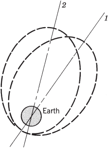
Figure 4–13 Shifting of the apsidal line of an elliptic orbit from position 1 to 2 because of the oblateness of the Earth.
Satellites of modern design, with irregular shapes due to protruding antennas, solar arrays, or other asymmetrical appendages, experience torques and forces that tend to perturb the satellite's position and orbit throughout its orbital life. Principal torques and forces result from the following factors:
- Aerodynamic drag. This factor is significant at orbital altitudes below 500 km and is usually assumed to cease at 800 km above the Earth. Reference 4–8 gives a detailed discussion of aerodynamic drag, which, in addition to affecting the attitude of unsymmetrical vehicles, causes a change in elliptical orbits known as apsidal drift, a decrease in the major axis, and a decrease in eccentricity of orbits about the Earth. See Refs. 4–6, 4–8, 4–12, and 4–13.
- Solar radiation. This factor dominates at high altitudes (above 800 km) and is due to impingement of solar photons upon satellite surfaces. The solar radiation pressure p (N/m2) on a given surface of the satellite in the vicinity of the Earth exposed to the sun can be determined from
where θ is the angle (in degrees) between the incident radiation vector and the normal to the surface and ks and kd are the specular and diffuse coefficients of reflectivity. Typical values are 0.9 and 0.5, respectively, for ks and kd on the body and antenna and 0.25 and 0.01, respectively, for ks and kd with solar array surfaces. Radiation intensity varies as the square of the distance from the sun (see Refs. 4–4 and 4–14). The torque T on the vehicle is given by
 , where A is the projected area normal to the flight direction (or normal to the sun's rays) and l is the offset distance between the spacecraft's center of gravity and the center of solar pressure. For a nonsymmetrical satellite with a large solar panel on one side, solar radiation will cause a small torque that will rotate the vehicle.
 - Gravity gradients. Gravitational torques in spacecraft result from variations in the gravitational force on the distributed mass of a spacecraft. Determination of this torque requires knowledge of the gravitational field and the distribution of spacecraft mass. This torque decreases as a function of the orbit radius and increases with the offset distances of masses within the spacecraft (including booms and appendages); it is most significant in large spacecraft or in space stations operating in relatively low orbits (see Refs. 4–4 and 4–15).
- Magnetic field. The Earth's magnetic field and any magnetic moment within the satellite can interact to produce torque. The Earth's magnetic field precesses about the Earth's axis but is very weak (0.63 and 0.31 gauss at poles and equator, respectively). This field is continually fluctuating in direction and intensity because of magnetic storms and other influences. Since the field strength decreases with 1/R3 with the orbital altitude, magnetic field forces are often neglected in the preliminary analysis of satellite flight paths (see Ref. 4–16).
- Internal accelerations. Deployment of solar array panels, the shifting of liquid propellants, the movement of astronauts or other masses within the satellite, or the “unloading” of reaction wheels may produce noticeable torques and forces.
- For precise low Earth orbits the oblateness of the Earth (diameter at equator being slightly larger than diameter between poles), high mountains, or Earth surface areas of different densities will cause perturbations of these orbits.
We can categorize satellite propulsion needs according to their function as listed in Table 4–2, which shows the total impulse “budget” applicable to a typical high‐altitude, elliptic orbit satellite. The control system designer often distinguishes two different kinds of station‐keeping orbit corrections needed to keep the satellite in a synchronous position. The east–west correction refers to a correction that moves the point at which a satellite orbit intersects the Earth's equatorial plane in an east or west direction; it usually corrects forces caused largely by the oblateness of the Earth. The north–south correction counteracts forces usually connected with the third‐body effects of the sun and the moon.
Table 4–2 Typical Propulsion Functions and Approximate Total Impulse Needs of a 2000‐lbm Geosynchronous Satellite with a Seven‐Year Life
| Function | Total Impulse (N‐sec) |
| Acquisition of orbit | 20,000 |
| Attitude control (rotation) | 4000 |
| Station keeping, E–W | 13,000 |
| Station keeping, N–S | 270,000 |
| Repositioning (Δu, 200 ft/sec) | 53,000 |
| Control apsidal drift (third‐body attraction) | 445,000 |
| Deorbit | 12,700 |
| Total | 817,700 |
For many satellite missions any gradual changes in orbit caused by perturbation forces are of little concern. However, in certain missions it is necessary to compensate for these perturbing forces and maintain the satellite in a specific orbit at a particular position in that orbit. For example, synchronous communications satellites in a Geosynchronous Earth Orbit, or GEO, need to maintain their position and their orbit so as to be able to (1) keep covering a specific area of the Earth or communicate with the same Earth stations within its line of sight and (2) not become a hazard to other satellites in this densely populated synchronous equatorial orbit. Another example is Low Earth Orbit or LEO communications satellites system with several coordinated satellites; here at least one satellite has to be in a position to receive and transmit radio‐frequency (RF) signals to specific locations on the Earth. The orbits and relative positions of several satellites with respect to each other also need to be controlled and maintained (see Ref. 4–3).
Orbit maintenance requires applying small correcting forces and torques periodically to compensate for perturbation effects; for GEO this happens every few months. Typical velocity increments for the orbit maintenance of synchronous satellites require a Δu between 10 and 50 m/sec per year. For a satellite mass of about 2000 kg a 50‐m/sec correction for a 10‐year orbit life would need a total impulse of about 100,000 N‐sec, which corresponds to a chemical propellant mass of 400 to 500 kg (about a quarter of the satellite mass) when done with small monopropellant or bipropellant thrusters. It would require much less propellant if electrical propulsion were to be used, but for some spacecraft the inert mass of the power supply and mission duration might represent a substantial increase . See Refs. 4–6, 4–13, and 4–14.
Mission Velocity
A convenient way to describe the magnitude of the energy requirement for a space mission is to use the concept of the mission velocity. It is the sum of all the flight velocity increments needed (in all the vehicle's stages) to attain the mission objective even though these increments are provided by different propulsion systems and their thrusts may be in different directions. In the sketch of a planetary landing mission of Fig. 4–11, it is the sum of all the Δu velocity increments shown by the heavy lines (rocket‐powered flight segments) of the trajectories. Even through some velocity increments might be achieved by retro‐action (a negative propulsion force to decelerate the flight velocity), all these maneuvers require energy and their absolute magnitude is counted in the mission velocity. The initial velocity from the Earth's rotation (464 m/sec at the equator and 408 m/sec at a launch station at 28.5° latitude) does not need to be provided by the vehicle's propulsion systems. For example, the required mission velocity for launching at Cape Kennedy, bringing the space vehicle into an orbit at 110 km, staying in orbit for a while, and then entering a deorbit maneuver has the Δu components shown in Table 4–3.
Table 4–3 Typical Estimated Space Shuttle Incremental Flight Velocity Breakdown for Flight to Low Earth Orbit and Return
| Ideal satellite velocity | 7790 m/sec |
| Δu to overcome gravity losses | 1220 m/sec |
| Δu to turn the flight path from the vertical | 360 m/sec |
| Δu to counteract aerodynamic drag | 118 m/sec |
| Orbit injection | 145 m/sec |
| Deorbit maneuver to reenter atmosphere and aerodynamic braking | 60 m/sec |
| Correction maneuvers and velocity adjustments | 62 m/sec |
| Initial velocity provided by the Earth's rotation at 28.5° latitude | −408 m/sec |
| Total required mission velocity | 9347 m/sec |
The required mission velocity is the sum of the absolute values of all translation velocity increments that have forces going through the center of gravity of the vehicle (including turning maneuvers) during the mission flight. It is the hypothetical velocity that would be attained by the vehicle in a gravity‐free vacuum, if all the propulsive energy of the momentum‐adding thrust chambers in all stages were to be applied in the same direction. This theoretical value is useful for comparing one flight vehicle design with another and as an indicator of total mission energy.
The required mission velocity must equal to the “supplied” mission velocity, that is, the sum of all the velocity increments provided by the propulsion systems during each of the various vehicle stages. The total velocity increment that was “supplied” by the Shuttle's propulsion systems for the Shuttle mission (solid rocket motor strap‐on boosters, main engines and, for orbit injection, also the increment from the orbital maneuvering system—all shown in Fig. 1–14) had to equal or exceed 9347 m/sec. When the reaction control system propellant and an uncertainty factor are added, this value would have needed to exceed 9621 m/sec. With chemical propulsion systems and a single stage, we can achieve space mission velocities of 4000 to 13,000 m/sec, depending on the payload, mass ratio, vehicle design, and propellant. With two stages they can be between perhaps 12,000 and 22,000 m/sec.
Rotational maneuvers (to be described later) do not change the flight velocity and some analysts do not add them to the mission velocity requirements. Also, maintaining a satellite in orbit against long‐term perturbing forces (see prior section) is often not counted as part of the mission velocity. However, designers need to provide additional propulsion capabilities for these purposes. These are often separate propulsion systems, called reaction control systems.
Table 4–4 Approximate Vehicle Mission Velocities for Typical Space and Interplanetary Missions
| Mission | Ideal Velocity (km/sec) | Approximate Actual Velocity (km/sec) |
| Satellite orbit around Earth (no return) | 7.9–10 | 9.1–12.5 |
| Escape from Earth (no return) | 11.2 | 12.9 |
| Escape from moon | 2.3 | 2.6 |
| Earth to moon (soft landing on moon, no return) | 13.1 | 15.2 |
| Earth to Mars (soft landing) | 17.5 | 20 |
| Earth to Venus (soft landing) | 22 | 25 |
| Earth to moon (landing on moon and return to Eartha) | 15.9 | 17.7 |
| Earth to Mars (landing on Mars and return to Eartha) | 22.9 | 27 |
aAssumes air braking within atmospheres.
Table 4–5 Approximate Relative Payload‐Mission Comparison Chart for Typical Multistage Rocket Vehicles Using Chemical Propulsion Systems
| Mission | Relative Payloada (%) |
| Earth satellite | 100 |
| Earth escape | 35–45 |
| Earth 24‐hr orbit | 10–25 |
| Moon landing (hard) | 35–45 |
| Moon landing (soft) | 10–20 |
| Moon circumnavigation (single fly‐by) | 30–42 |
| Moon satellite | 20–30 |
| Moon landing and return | 1–4 |
| Moon satellite and return | 8–15 |
| Mars flyby | 20–30 |
| Mars satellite | 10–18 |
| Mars landing | 0.5–3 |
a300 nautical miles (555.6 km) Earth orbit is 100% reference.
Typical vehicle velocities required for various interplanetary missions have been estimated as shown in Table 4–4. By starting interplanetary journeys from a space station, considerable savings in vehicle velocity can be achieved, namely, the velocity necessary to attain the Earth‐circling satellite orbit. As space flight objectives become more ambitious, mission velocities increase. For a given single or multistage vehicle it is possible to increase the vehicle's terminal velocity, but usually only at the expense of payload. Table 4–5 shows some typical ranges of payload values for a given multistage vehicle as a percentage of a payload for a relatively simple Earth orbit. Thus, a vehicle capable for putting a substantial payload into a near‐Earth orbit can only land a very small fraction of this payload on the moon, since it has to have additional upper stages, which displace payload mass. Therefore, much larger vehicles are required for space flights with high mission velocities when compared to a vehicle of less mission velocity but identical payload. The values listed in Tables 4–4 and 4–5 are only approximate because they depend on specific vehicle design features, the propellants used, exact knowledge of the trajectory–time relation, and other factors that are beyond the scope of this abbreviated treatment.
4.5 SPACE FLIGHT MANEUVERS
Ordinarily, all propulsion operations are controlled (started, monitored, and stopped) through the vehicle's guidance and control system. The following types of space flight maneuvers and vehicle accelerations utilize rocket propulsion:
- The propulsion systems in the first stage and strap‐on booster stage add momentum during launch and ascent of the space vehicles. They require high or medium level thrust of limited durations (typically 0.7 to 8 min). To date all Earth‐launch operations have used chemical propulsion systems and these constitute the major mass portion of the space vehicle; they are discussed further in the next section.
- Orbit injection is a powered maneuver that adds velocity to the top stage (or payload stage) of a launch vehicle, just as it reaches the apogee of its ascending elliptical trajectory. Figure 4–10 shows the ascending portion of such elliptical flight path which the vehicle follows up to its apogee. The horizontal arrow in the figure symbolizes the application of thrust in a direction such as to inject the vehicle into an Earth‐centered coplanar orbit. This is performed by the main propulsion system in the top stage of the launch vehicle. For injection into a low Earth orbit, thrust levels are typically between 200 and 45,000 N or 50 and 11,000 lbf, depending on the payload size, transfer time, and specific orbit.
- A space vehicle's transfer from one orbit to another (coplanar) orbit has two stages of rocket propulsion operation. One operates at the beginning of the transfer maneuver from the launching orbit and the other at the arrival at the destination orbit. The Hohmann ellipse shown in Figure 4–9 gives the most energy efficient transfer (i.e., the smallest amount of propellant usage). Reaction control systems are used here to orient the transfer thrust chamber into a proper direction. If the new orbit is higher, then thrusts are applied in the flight direction. If the new orbit is at a lower altitude, then thrusts must be applied in a direction opposite to the flight velocity vector. Transfer orbits can also be achieved with a very low thrust level (0.001 to 1 N) using an electric propulsion system, but flight paths will be very different (multiloop spirals) and transfer durations will be much longer, (see Chapter 17). Similar maneuvers are also performed with lunar or interplanetary flight missions, such as the planetary landing mission shown schematically in Fig. 4–11.
- Velocity vector adjustment and minor in‐flight correction maneuvers for both translation and rotation are usually performed with low‐thrust, short‐duration, intermittent (pulsing) operations using a reaction control system with multiple small liquid propellant thrusters. Vernier rockets on ballistic missiles are used to accurately calibrate its terminal velocity vector for improved target accuracy. Reaction control rocket systems on a space launch vehicle will allow for accurate orbit‐injection adjustment maneuvers after it has been placed into orbit by its other, less accurate, propulsion systems. Midcourse guidance‐directed correction maneuvers for the trajectories of deep space vehicles similarly fall into this category. Propulsion systems for orbit maintenance maneuvers, also called station‐keeping maneuvers (for overcoming perturbing forces), that keep spacecraft in their intended orbit and orbital position are also considered to be in this category.
- Reentry and landing maneuvers may take several forms. If landing occurs on a planet that has an atmosphere, then drag in that atmosphere will heat and slow down the reentering vehicle. For multiple elliptical orbits, drag will progressively reduce the perigee altitude and the perigee velocity at every orbit. Landing at a precise or preplanned location requires a particular velocity vector at a predetermined altitude and distance from the landing site. The vehicle has to be rotated into a proper position and orientation so as to use its decelerators and heat shields correctly. Precise velocity magnitudes and directions prior to entering any denser atmosphere are critical for minimizing heat transfer (usually to a vehicle's heat shield) and to achieve touchdown at the intended landing site or, in the case of ballistic missiles, the intended target and this commonly requires a relatively minor maneuver (of low total impulse). If there is very little or no atmosphere (for instance, landing on the moon or Mercury), then an amount of reverse thrust has to be applied during descent and at touchdown. Such rocket propulsion system needs to have a variable thrust capability to assure a soft landing and to compensate for the decrease in vehicle mass as propellant is consumed during descent. The U.S. lunar landing rocket engine, for example, had a 10 to 1 thrust variation.
- Rendezvous and docking between two space vehicles involve both rotational and translational maneuvers with small reaction control thrusters. Docking (sometimes called lock‐on) is the linking up of two spacecraft and requires a gradual gentle approach (low thrust, pulsing‐mode thrusters) so as not to cause spacecraft damage.
- Simple rotational maneuvers rotate the vehicle on command into a specific angular position in order to orient/point a telescope or other instrument (a solar panel, or an antenna for purposes of observation, navigation, communication, or solar power receptor). Such a maneuver is also used to keep the orientation of a satellite in a specific direction; for example, if an antenna needs to be continuously pointed at the center of the Earth, then the satellite needs to be rotated around its own axis once every satellite revolution. Rotation is also used to point nozzles in the primary propulsion system into their intended direction just prior to their operation. The reaction control system can also provide pulsed thrusting; it has been used for achieving flight stability, and/or for correcting angular oscillations that would otherwise increase drag or cause tumbling of the vehicle. Spinning or rolling a vehicle about its axis will not only improve flight stability but also average out thrust vector misalignments. Chemical multithruster reaction‐control systems are used when rotation needs to be performed quickly. When rotational changes may be done over long periods of time, electrical propulsion systems (operating at a higher specific impulse) with multiple thrusters are often preferred.
- Any change of flight trajectory plane requires the application of a thrust force (through the vehicle's center of gravity) in a direction normal to the original flight‐path plane. This is usually performed by a propulsion system that has been rotated (by its reaction control system) into the proper nozzle orientation. Such maneuvers are done to change a satellite orbit's plane or when traveling to a planet, such as Mars, whose orbit is inclined to the plane of the Earth's orbit.
- Deorbiting and disposal of used or spent rocket stages and/or spacecraft is an important requirement of increasing consequences for removing space debris and clutter. Spent spacecraft must not become a hazard to other spacecraft or in the event of reentry threaten population centers. Relatively small thrusts are used to drop the vehicle to a low enough elliptical orbit so that atmospheric drag will slow down the vehicle at the lower elevations. In the denser regions of the atmosphere during reentering, expended vehicles will typically break up and/or overheat (and burn up). Ground based energetic lasers and in‐space debris removers are also being considered. International efforts will be required to solve this fast growing “space junk” problem.
- Emergency or alternative mission. When there is a malfunction in a spacecraft and it is decided to abort the mission, such as a premature quick return to the Earth without pursuing the originally intended mission, then specifically suitable rocket engines can be used for such alternate missions. For example, the main rocket engine in the Apollo lunar mission service module was normally used for retroaction to attain a lunar orbit and for return from lunar orbit to the Earth; it could also have been used for emergency separation of the payload from the launch vehicle and for unusual midcourse corrections during translunar coast, enabling an emergency Earth return.
Table 4–6 lists all maneuvers that have just been described, together with some others, and shows the various types of rocket propulsion system (as introduced in Chapter 1) that have been used for each of these maneuvers. The table omits several propulsion systems, such as solar thermal or nuclear rocket propulsion, because these have not yet flown in routine space missions. One of the three propulsion systems on the right of Table 4–6 is electrical propulsion which has relatively high specific impulse (see Table 2–1), and this makes it very attractive for deep space missions and for certain station‐keeping jobs (orbit maintenance). However, electrical thrusters perform best when applied to missions where sufficiently long thrust action times for reaching the desired vehicle velocity or rotation positions are available because of their very relatively small accelerations.
Table 4–6 Types of Rocket Propulsion Systems Commonly Used for Different Flight Maneuvers or Application
| Liquid Propellant Rocket Engines | Solid Propellant Rocket Motors | Electrical Propulsion | ||||||

|
High Thrust, Liquid Propellant Rocket Engine, with Turbopump | Medium to Low Thrust, Liquid Propellant Rocket Engine | Pulsing Liquid Propellant, Multiple Small Thrusters | Large Solid Propellant Rocket Motor, Often Segmented | Medium to Small Solid Propellant Motors | Arcjet, Resistojet | Ion Propulsion, Electromagnetic Propulsion | Pulsed Plasma Jet |
| Launch vehicle booster | × × | × × | ||||||
| Strap‐on motor/engine | × × | × × | ||||||
| Upper stages of launch vehicle | × × | × × | × | × × | ||||
| Satellite orbit injection and transfer orbits | × × | × × | × | × | ||||
| Flight velocity adjustments, flight path corrections, orbit changes | × | × × | × | × | ||||
| Orbit/position maintenance, rotation of spacecraft | × × | × | × | × | ||||
| Docking of two spacecraft | × × | |||||||
| Reentry and landing, emergency maneuvers | × | × | × | |||||
| Deorbit | × | × | × | × | ||||
| Deep space, sun escape | × | × | × | |||||
| Tactical missiles | × × | |||||||
| Strategic missiles | × | × | × | × × | × × | |||
| Missile defense | × | × × | × × | |||||
| Artillery shell boost | × × | |||||||
Legend: × = in use: × × = preferred for use in recent years.
During high‐speed atmospheric reentry vehicles encounter extremely high heating loads. In the Apollo program a heavy thermal insulation layer was located at the bottom of the Apollo Crew Capsule and in the Space Shuttle Orbiter low‐conductivity, lightweight bricks on the wings provided thermal protection to the vehicle and crew. An alternate method in multi‐engine main rocket propulsion vehicles is to reduce high Earth reentry velocities by reversing or retro directing the thrust of some of the engines. This requires to turn the vehicle around in space by 180° (usually by means of several attitude control thrusters) prior to the return maneuver and then firing the necessary portion of the main propulsion system. An example of this method can be found in the Falcon 9 Space Vehicle booster stage reentry, the lower portion of which is shown in the front cover of this book. The aim here is simply to recover and reuse this stage. All nine (9) Merlin liquid propellant rocket engines are needed during ascent to orbit but only 3 of these are sufficient for the retro‐slowdown maneuver during reentry, and only the central engine need be operated during the final vertical landing maneuver. Before reusing and relaunching, the recovered booster stage with its multiple rocket engines is refurbished—all residual propellant is removed and the unit is cleaned, flushed, and purged with hot dry air. Upon inspection, further maintenance may be performed as needed. Since the booster stage is usually the most expensive stage, this reuse will allow some cost reduction (if used often enough).
Reaction Control System
All functions of a reaction control system have been described in the previous section on flight maneuvers; they are used for the maneuvers identified by paragraphs d, f, and h. In some vehicle designs they are also used for tasks described in b and c, and parts of e and g, if the thrust levels are low.
A reaction control system (RCS), often also called an auxiliary rocket propulsion system, is needed to provide trajectory corrections (small Δu additions) as well as for correcting rotational or attitude positions in almost all spacecraft and all major launch vehicles. If mostly rotational maneuvers are made, the RCS has been called an attitude control system (but this nomenclature is not consistent throughout the industry or the literature).
An RCS is usually incorporated into the payload stage and into each of the stages of a multiple‐stage vehicle. In some missions and designs the RCS is only built into the uppermost stage; it operates throughout the flight and provides needed control torques and forces for all the stages. In large vehicle stages, thrust levels of multiple thrusters of an RCS are correspondingly large (500 to 15,000 lbf), and for terminal stages in small satellites they can be small (0.01 to 10.0 lbf) and may be pulsed. Liquid propellant rocket engines with multiple thrusters are presently used in nearly all launch vehicles and in most spacecraft. Cold gas systems were used exclusively with early spacecraft. In the last two decades, an increasing number of electrical propulsion systems are being used, primarily on spacecraft (see Chapter 17). The life of an RCS may be short (when used on an individual vehicle stage) or it may be used throughout the mission duration (some more than 10 years) when part of an orbiting spacecraft.
Vehicle attitude has to be controlled about three mutually perpendicular axes, each with two degrees of freedom (clockwise and counterclockwise rotation), giving a total of six degrees of freedom. Pitch control raises or lowers the nose of the vehicle, yaw torques induce motion to the right or left side, and roll torques will rotate the vehicle about its axis, either clockwise or counterclockwise. In order to apply a pure torque it is necessary to use two thrust chambers of equal thrust and equal start and stop times, placed equidistant from the center of mass. Figure 4–14 shows a simple spherical spacecraft attitude control system; thrusters x − x or x′ − x′ apply torques that rotate about the X axis. There should be a minimum of 12 thrusters in such a system, but some spacecraft with geometrical or other limitations on the placement of these nozzles or with provisions for redundancy may actually have more than 12. The same system can, by operating different sets of nozzles, also provide translation forces; for example, if one each of the (opposite) thrust units x and x′ were operated simultaneously, the resulting forces would propel the vehicle in the direction of the Y axis. With clever designs it is possible to use fewer thrusters, but they will usually not provide a pure torque.

Figure 4–14 Simplified attitude control system diagram for spacecraft. It requires 12 thrusters (identified as x, y, z pairs) to allow the application of pure torques about three perpendicular axes. The four unlabeled thrusters, shown at the top and bottom clusters, would be needed for translation maneuvers along the Z axis.
An RCS usually contains the following major subsystems: (1) sensing devices for determining the attitude, velocity, and/or position of the vehicle with respect to some reference direction at any given time, such as provided by gyroscopes, star‐trackers, or radio beacons; (2) a control‐command system that compares the actual space and rotary position with the desired or programmed position and issues command signals to change the vehicle's position within a desired time period; and (3) devices for changing the angular position, such as a set of high‐speed gyroscopic wheels or sets of RCS or small attitude control thrusters. See Refs. 4–13 and 4–14.
Precise attitude angular corrections can also be achieved by the use of inertial or high‐speed rotating reaction wheels, which apply torques when their rotational speed is increased or decreased. While these wheels are quite simple and effective, the total amount of angular momentum change they can supply is limited. By using pairs of supplementary attitude control thrust rocket units, it is possible to unload or even respin each wheel so it can continue to supply small angular position corrections as needed.
The torque T of a pair of thrust chambers of thrust F and separation distance l provides the vehicle with an angular or rotational moment of inertia Ma an angular acceleration of magnitude α:
For a cylinder of radius r and of equally distributed mass the rotational moment of inertia is ![]() and for a homogeneous sphere it is
and for a homogeneous sphere it is ![]() . The largest possible practical value of moment arm l will minimize thrust and propellant requirements. If the angular acceleration is constant over a time t, the vehicle will move at an angular speed ω and through a displacement angle θ, namely,
. The largest possible practical value of moment arm l will minimize thrust and propellant requirements. If the angular acceleration is constant over a time t, the vehicle will move at an angular speed ω and through a displacement angle θ, namely,
Commonly, the control system senses a small angular disturbance and then commands an appropriate correction. For detection of angular position changes by an accurate sensor, it is usually necessary for the vehicle to undergo a slight angular displacement. Care must be taken to avoid overcorrection and hunting of the vehicle's position by the control system. This is one of the reasons many spacecraft use extremely short multiple pulses (0.010 to 0.040 sec per pulse) and low thrust (0.01 to 100 N) (see Refs. 4–11, 4–13 and 4–14).
Reaction control systems may be characterized by the magnitude of the total impulse and by the number, thrust level, and direction of the thrusters and their duty cycles. The duty cycle refers to the number of thrust pulses, their operating times, times between thrust applications, and timing of short operations during the mission operating period. For any given thruster, a 30% duty cycle would mean an average active cumulative thrust period of 30% during the propulsion system's flight duration. These propulsion parameters can be determined from the mission, the guidance and control approach, the desired accuracy, flight stability, the likely thrust misalignments of the main propulsion systems, the three‐dimensional flight path variations, the perturbations to the trajectory, and several other factors. Some of these parameters can often be difficult to determine.
4.6 EFFECT OF PROPULSION SYSTEM ON VEHICLE PERFORMANCE
This section gives several methods for improving flight vehicle performance and most of enhancements listed are directly influenced by the flight mission and by the selection or design of the vehicle and the propulsion system. Only a few flight vehicle performance improvements do not depend on the propulsion system. Most of those listed below apply to all missions, but some are peculiar to some missions only.
- The effective exhaust velocity c or its equivalent the specific impulse Is usually have a direct effect on the vehicle's overall performance. The vehicle's final velocity increment Δu may be increased by a higher Is. This can be done by using more energetic chemical propellants (see Chapters 7 and 12), by higher chamber pressures and, for upper stages operating at high altitudes, also by larger nozzle area ratios provided that all these do not appreciably increase the vehicle's inert mass. With electrical propulsion a higher available Is can enhance vehicle performance but, as explained in Chapter 17, their very low thrusts do limit their use to certain space missions.
- The vehicle mass ratio's (m0/mf) logarithmic effect can be increased in several ways. One way is by reducing the final mass mf (which consists of the inert hardware and payload plus the nonusable, residual propellant mass). Reducing the inert mass implies lighter structures, smaller payloads, lighter guidance/control devices, and/or less unavailable residual propellant; this often means going to stronger structural materials at higher stresses, more efficient power supplies, or smaller electronic packages. During design, there is always great emphasis on reducing all hardware and residual propellant masses to their practical minima. Another way is to increase the initial vehicle mass, and use higher thrust and more propellant, but with accompanying small increases in the structure or inert propulsion system mass.
- Reducing the burning time (i.e., increasing the thrust level) will reduce the gravitational loss in some applications. However, higher accelerations usually require more structural and propulsion system mass, which in turn cause the mass ratio to be less favorable.
- Atmospheric drag, which can be considered as negative thrust, can be reduced in at least four ways. Drag has several components: (a) Form drag depends on the flight vehicle's aerodynamic shape; slender pointed noses or sharp, thin leading edges on fins or wings have less drag than stubby, blunt shapes. (b) A vehicle with a small cross‐sectional area has less drag; propulsion designs that can be packaged in long, thin shapes will be preferred. (c) Drag is proportional to the cross‐sectional or frontal vehicle area; higher propellant densities will decrease propellant volume and therefore will allow smaller cross sections. (d) Skin drag is caused by the friction of the gas flowing over all vehicle's outer surfaces; smooth contours and polished surfaces are preferred; skin drag also depends on higher propellant densities because they require smaller volumes and thus lower surface areas. (e) Base drag is the fourth component; it is a function of the ambient pressure acting over the surface of the vehicle's base or rear section; it is influenced by the nozzle exit gas pressure and turbulence, any discharges of turbine exhaust gases, and by the geometry of the vehicle base design. These are discussed further in Chapter 20.
- The length of the propulsion nozzle is often a significant contributor to the overall vehicle or stage length. As described in Chapter 3, for each mission there is an optimum nozzle contour and length, which can be determined by trade‐off analyses. A shorter nozzle length or multiple nozzles on the same propulsion system may allow a somewhat shorter vehicle; in many designs this implies a somewhat lighter vehicle structure and a slightly better vehicle mass ratio.
- The final vehicle velocity at propulsion termination can be increased by increasing the initial velocity u0. By launching a satellite in an eastward direction the rotational speed of the Earth adds to the final satellite orbital velocity. This Earth tangential velocity is as high as 464 m/sec or 1523 ft/sec at the equator; Sea Launch, a commercial enterprise, launched from a ship at the equator to take full advantage of this velocity increment. For an easterly launch at John F. Kennedy Space Center (latitude of 28.5° north) this extra velocity is less, about 408 m/sec or 1340 ft/sec. Conversely, a westerly satellite launch has a negative initial velocity and thus requires higher‐velocity increments. Another way to increase u is to launch a spacecraft or an air‐to‐surface missile from a satellite or an aircraft, which imparts its initial vehicle velocity vector and allows launching in the desired direction. An example is the Pegasus three‐stage space vehicle, which is launched from an airplane.
- For vehicles that fly within the atmosphere it is possible to increase their range when aerodynamic lift is used to counteract gravity and reduce gravity losses. Using a set of wings and flying at an angle of attack increases the lift, but also adds to the drag. Vehicle lift may also be used to increase the maneuverability and trajectory flexibility.
- When the vehicle's flight velocity u is close to the rocket's effective exhaust velocity c, the propulsive efficiency is highest (Eq. 2–22 or Fig. 2–3) and more of the rocket exhaust gas energy is transformed into the vehicle's flight energy. When u = c this propulsive efficiency reaches 100%. Trajectories where u is close in value to c for a major portion of the flight therefore would need less propellant.
- When a mission is changed during flight, the liquid propellant of a particular rocket engine (in a multistage vehicle) may not be fully used and such unused propellant is then available to be transferred within the vehicle to augment the propellant of a different rocket engine system unit. An example was the transfer of storable liquid propellant in the Space Shuttle from the Orbital Maneuvering System (OMS) to the Reaction Control System (RCS – 14 small bipropellant thrusters). This transfer allowed for additional orbit maintenance operations and more time in orbit.
Several of these influencing parameters can be optimized. Therefore, for every mission or flight application there is an optimum propulsion system design and the propulsion parameters that define the optimum condition are dependent on vehicle or flight parameters.
4.7 FLIGHT VEHICLES
As previously stated, a vast majority of rocket‐propelled vehicles use a relatively simple single‐stage design and commonly employ solid propellant rocket motors. Most are used in military applications as described in the next section. In this section we discuss the more sophisticated multistage space launch vehicles and mention others, such as large ballistic missiles (often called strategic missiles) and some sounding rockets. All these require some intelligence acquisition for their guidance and must include navigation‐system hardware.
A single stage to orbit vehicle (e.g., to LEO) is very limited in the payload it can carry and this concept has been only of research interest. Figures 4–2 and 4–3 indicate that a high‐performance single‐stage vehicle with a propellant fraction of 0.95 and an average Is of 400 sec may achieve an ideal terminal velocity of nearly 12,000 m/sec without payload. If the analysis includes drag and gravity forces, a correspondingly higher value of Is would be needed. Accounting for maneuvers in the trajectory and an attitude control system, depending on design it is likely that a single stage's payload would remain at about 1.0% of the gross takeoff mass. For typical larger payload percentages and particularly for more ambitious missions, we use vehicles with two or more stages as described below.
Multistage Vehicles
Multistep or multistage rocket vehicles permit higher vehicle velocities, more payload for space vehicles, larger area coverage for defensive missiles, and improved performance for long‐range ballistic missiles or area defense missiles. After the useful propellant has been consumed in a particular stage, the remaining empty mass of that expended stage is dropped from the vehicle and the operation of the propulsion system of the next step or stage is started. The last or top stage, which is usually the smallest, carries the payload. Separating the empty mass of expended stages from the remainder of the vehicle avoids additional energy expenditures. As the number of stages is increased, the initial takeoff mass can decrease, but the relative gains in lowering initial mass become less and less with each additional stage. Moreover, adding stages increases the required physical mechanisms increasing vehicle complexity and total mass. The most economically useful number of stages is usually between two and six, depending on the mission. See Example 4–3. Several different multistage launch vehicle configurations have been used successfully, and four are shown in Fig. 4–15. Most vehicles are launched vertically, but a few have been otherwise launched from airplanes, such as the three‐stage Pegasus space vehicle.

Figure 4–15 Schematic renditions of four different geometric configurations for assembling individual stages into a launch vehicle.
Even though it represents only a very small portion of the initial mass, the payload of a multistage rocket is roughly proportional its takeoff mass. If a payload of 50 kg requires a 6000‐kg multistage rocket, a 500‐kg payload would require approximately a 60,000‐kg rocket unit with identical number of stages and similar configuration, using the same payload fraction and the same propellants. When the operation of an upper stage is started immediately after thrust termination of a lower stage, then the total ideal velocity of a multistage vehicle with purely series‐stage (or tandem) arrangement is simply the sum of the individual stage velocity increments. For n stages in series as shown in the first sketch of Fig. 4–15 the final velocity increment Δuf is
In vertical atmospheric flight, the individual velocity increments are each given by Eq. 4–19. For the simplified case of a vacuum flight in a gravity‐free field this equation may be expressed as (applying Eq. 4–6)
This equation defines the maximum velocity that an ideal multistage vehicle in a tandem configuration may attain. It assumes a space environment (no drag or gravity) and that the upper stage propulsion system starts at full thrust exactly when the lower stage stops (no time delays) without any of the common thrust declines at shutdown In atmospheric trajectories because the actual stage separation process has some unavoidably small delays (with very low or no thrust), the individual velocity increments in Eq. 4–35 need to be determined by integrating Eqs. 4–15 and 4–16 which are more general and consider drag and gravity losses; this is discussed in the next subsection. Other losses or trajectory perturbations can also be included as mentioned earlier in this chapter, but such an approach requires numerical solutions.
For two‐ or three‐stage vehicles the overall vehicle mass ratio (initial mass at takeoff to final mass of last stage) can reach values of over 100. Figure 4–2 may be separated into regions applicable to each stage, such as single‐stage vehicles (with 1/![]() ≤ 95) and tandem or multistage vehicles (with 1/
≤ 95) and tandem or multistage vehicles (with 1/![]() up to and beyond 180). Equation 4–36 does not apply to the parallel, partial or piggy back staging identified in Fig. 4–15. For such stages where more than one propulsion system is operating at the same time and producing thrust in the same direction, the overall specific impulse, overall propellant mass flow and overall thrust and mass flow are given by Eqs. 2–23 to 2–25 or 11–1 to 11–3.
up to and beyond 180). Equation 4–36 does not apply to the parallel, partial or piggy back staging identified in Fig. 4–15. For such stages where more than one propulsion system is operating at the same time and producing thrust in the same direction, the overall specific impulse, overall propellant mass flow and overall thrust and mass flow are given by Eqs. 2–23 to 2–25 or 11–1 to 11–3.
The first sketch in Fig. 4–15 depicts a common configuration where the stages are stacked vertically on top of each other, as in the Minuteman long‐range missile or the Russian Zenit (or Zenith) launch vehicle. Partial staging was used on the early versions of the U.S. Atlas vehicle; it allowed all engines to be started together, thus avoiding an altitude start for the sustainer engine, which was unproven in those early days; the two Atlas booster engines arranged in a doughnut‐shaped assembly were dropped off in flight. The third sketch in Fig. 4–15 has two or more separate booster “strap‐on” stages attached to the bottom stage of a vertical configuration (they can be either solid or liquid propellants) and this allows for increases in vehicle capability. The piggyback configuration concept on the right was used on the Space Shuttle—its two large solid rocket motor boosters are shown in Fig. 1–14.
Stage Separation
It takes a finite time for the thrust termination of a lower stage propulsion system to go to essentially zero (typically 1 to 3 sec for large thruster chambers and for small thrusters as brief as 1 msec). In some multistage flight vehicles (with stage separation devices), there can be further delays (about 4 to 10 sec) to achieve a respectable separation distance between stages before firing the upper stage propulsion system can be initiated. This is needed in order to prevent any blow‐back or damage from hot flames onto the upper stage. Also, upper stage engine start‐ups are not instantaneous but require one or more seconds in larger rocket propulsion systems. During these several‐second cumulative delays, the Earth's gravity pull acts to diminish the vehicle's upward velocity, causing a reduction of the flight velocity by perhaps 20 to 500 ft/sec (7 to 160 m/sec). A scheme called hot staging has been introduced to diminish this velocity loss and shorten staging time intervals—the upper stage propulsion system is actually started at a low but increasing thrust before the lower stage propulsion system has been fully shut off or well before it reaches essentially zero thrust; special flame‐resistant ducts are placed in the interstage structure to allow the hot exhaust gases from the upper stage engine to be symmetrically deflected and safely discharged prior to and immediately after the actual separation of the stages. Because this improves flight performance, hot staging schemes have been used in large multistage vehicles such as the Titan II in the United States and in certain Chinese and Russian launch vehicles.
For multistage vehicles the stage mass ratios, thrust levels, propulsion durations, and location or travel of the center of gravity of the stages are all usually optimized, often using complex trajectory computer programs. High specific impulse chemical rocket engines (e.g., those using hydrogen–oxygen propellants) are normally employed in upper stages of space launch vehicles because here any small increase in specific impulse can be usually more effective than in the lower stages.
If a three‐stage vehicle had been used in Example 4–3 instead two, the theoretical payload increase will add only about 8 or 10%. A fourth stage gives an even smaller theoretical improvement; it would add only 3 to 5% to the payload. Hence, the potential amount of performance improvement diminishes with each added stage. Moreover, each additional stage means extra complexity in an actual vehicle (such as a reliable separation mechanism, an interstage structure, more propulsion systems, joints or couplings in connecting pipes and cables, etc.), requires additional inert mass (increasing the mass ratio ![]() ), and compromises the overall reliability. Therefore, the minimum number of stages that will meet the payload and Δu requirements is usually selected.
), and compromises the overall reliability. Therefore, the minimum number of stages that will meet the payload and Δu requirements is usually selected.
The flight paths taken by the vehicles in the two simplified cases of Example 4–3 have to be different because their time of flight and the acceleration histories are different. One conclusion from this example that applies to all multistage rocket‐propelled vehicles is that for each mission there is an optimum number of stages, an optimum distribution of the mass between the stages, and usually also an optimum flight path for each design, where key vehicle parameters such as payload, velocity increment, or range are maximized.
Launch Vehicles
The first or lowest stage, often called a booster stage, is usually the largest and requires the largest thrust and largest total impulse. For Earth surface launches, all stages presently use chemical propulsion to achieve desired thrust‐to‐weight ratios. Thrust magnitudes decrease with each subsequent stage, also known as the upper or sustainer stages. Thrust requirements depend on the total mass of the vehicle, which in turn depend on the mass of the payload and on the mission. Typical configurations are shown in the sketches of Fig. 4–15.
Many launch vehicles with large payloads have between one and six large strap‐on stages, also called “zero stages or half stages.” These augment the thrust of the booster stage; all units are usually started at the same time. A schematic diagram is shown as the parallel staging sketch in Fig. 4–15. Solid propellant strap‐on stages are common, such as the Atlas V shown in Fig. 1–13 or the Space Shuttle shown in Fig. 1–14. These strap‐on stages are usually smaller in size than their equivalent liquid propellant units (due to higher propellant density) and have less drag but may produce a very toxic exhaust. Liquid propellant strap‐on stages are used in the Delta IV Heavy lift launch vehicle (see Fig. 1–12), and have been used in the first Soviet ICBM (intercontinental ballistic missile, circa 1950) and in several Soviet/Russian space launch vehicles. Most deliver higher specific impulse than their solid propellant counterparts and enhance vehicle performance but require propellant filling at the launch site.
There is some variety in existing launch vehicles. The smaller ones are for low payloads and low orbits; the larger ones usually have more stages, are heavier, and have larger payloads or higher mission velocities. Vehicle cost increases with the number of stages and with initial vehicle launch mass. Once a particular launch vehicle has proven to be reliable, it is often modified and uprated to allow for improvements in its capability or mission flexibility. Each stage of a space launch vehicle can have several rocket engines, each for specific missions or maneuvers. The Space Shuttle system, shown in Fig. 1–14, had 67 different rocket propulsion systems. In most cases each rocket engine was used for a single maneuver, but in some cases the same engine could be used for more than one specific purpose; the small reaction control thrusters in the Shuttle, for example, served to give attitude control (pitch, yaw, and roll) during orbit insertion and reentry, for counteracting internal shifting of masses (astronaut movement, extendible arm), small trajectory corrections, minor flight path adjustments, docking, and for the precise pointing of scientific instruments.
The spacecraft is that portion of a launch vehicle that carries the payload. It is the only part of the vehicle that goes into orbit or into deep space and/or returns to Earth. Final major space maneuvers, such as orbit injection or planetary landing, often require substantial velocity increments; the propulsion system, which provides the force for such maneuvers, may be integrated with the spacecraft or may be part of a discardable stage, just below the spacecraft. Several of the maneuvers described in Section 4.5 may often be accomplished by propulsion systems located in two different stages of a multistage vehicle. The selection of the most desirable propulsion systems, together with the decision of which of the several propulsion systems will perform specific maneuvers, will depend on optimizing performance, cost, reliability, schedule, and mission flexibility as further described in Chapter 19.
When a space vehicle is launched from the Earth's surface into orbit, it flies through three distinct trajectory phases: (1) Most are usually launched vertically and then undergo a turning maneuver while under rocket power to point the flight velocity vector into the desired direction; (2) the vehicle then follows a free‐flight (unpowered) ballistic trajectory (usually elliptical), up to its apex; finally, (3) satellites would need an extra push from a rocket propulsion system to add enough total impulse or energy to accelerate to orbital velocity. This last maneuver is also known as orbit insertion or sometimes as a kick maneuver. During the initial powered flight, the trajectory angle and the thrust cutoff velocity of the last stage are adjusted by the guidance system to a velocity vector in space that will allow the vehicle to reach the apogee of its elliptic path exactly at the desired orbit altitude. As shown in Fig. 4–10, a multistage ballistic missile follows the same two ascent flight phases mentioned above, but it then continues its elliptical ballistic trajectory going down to its target.
Historically, launch vehicles have been successfully modified, enlarged, and improved in performance. Newer versions retain most of the old, proven, reliable components, materials, and subsystems. This reduces development efforts and costs. Upgrading a vehicle allows for an increase in mission energy (i.e., more ambitious missions) or payload or both. Typically, this is done by one or more of following types of improvement: increasing the mass of propellant without an undue increase in tank or case mass; uprating the thrust and strengthening the engine; increasing the specific impulse; or adding successively more or bigger strap‐on boosters. Upgrading also usually requires a strengthening of the structure to accept higher loads.

Figure 4–16 Changes of payload with circular orbit altitude and orbit inclination for early version of the airplane‐launched Pegasus launch vehicle. This is a relatively simple three‐stage launch vehicle of 50 in. diameter driven by a solid propellant rocket motor in each stage.
Courtesy Orbital ATK
Figure 4–16 shows effects of orbit inclination and altitude on payload capability of the Pegasus (a relatively small, airplane‐launched space launch vehicle). Inclination is the angle between the equatorial plane of the Earth and the trajectory; an equatorial orbit has zero inclination and a polar orbit has 90° inclination. Since the Earth's rotation gives the vehicle an initial velocity, launching from the equator in an eastward direction will give the highest payload. For the same orbit altitudes other trajectory inclinations have lower payloads. For the same inclinations, payload decreases with orbit altitude since more energy has to be expended to overcome gravitational attraction. The figure shows that a practical payload becomes too small for orbits higher than about 1200 km. To lift heavier payloads and to go to higher orbits requires a larger launch vehicle than Pegasus vehicle. Figure 4–16 is based on the assumption of a particular payload separation length (38 in.) and a specific Δu vehicle velocity reserve (220 ft./sec) for variables such as the normal changes in atmospheric density (which can double the drag) or the mass tolerances of the propulsion systems. Similar curves are produced by the makers of other launch vehicles.
The Space Shuttle achieved its maximum payload when launched due east into an orbit with 28.5° inclination from Kennedy Space Flight Center in Florida, namely about 56,000 lbm (or 25,402 kg) at a 100‐nautical‐mile (185‐km) orbit altitude. Such payload decreased by about 100 lbm (45.4 kg) for every nautical mile increase in altitude. When the inclination is 57°, the payload diminishes to about 42,000 lbm (or 19,051 kg). If launched in a southerly direction from Vandenberg Air Force Base on the U.S. West Coast in a 98° inclination into a circular, nearly polar orbit, the payload will be only about 30,600 lbm or 13,880 kg.
4.8 MILITARY MISSILES
A majority of all rocket propulsion systems built today is used for military purposes. There is a large variety of missiles, projectiles and military missions and therefore many different propulsion systems, all using chemical propulsion systems. They range from simple, small, unguided, fin‐stabilized, single‐stage rocket projectiles (used in air‐to‐surface missions and surface‐to‐surface bombardment) up to complex, sophisticated, expensive, long‐range, multistage ballistic missiles (intended for faraway military or strategic targets). The term surface means not only land surface (ground launch or ground target) but also ocean surface (ship launched) and below ocean surface (submarine launched). A tactical missile can be used for attacking or defending ground troops, nearby military or strategic installations, military aircraft, short‐range missiles, and/or antitank missiles. Armed forces also use military satellites for missions such as reconnaissance, early warning of impending attack, secure communication (including command and control) and to accurately locate particular items on the Earth's surface (latitude and longitude).
Strategic missiles with a range of 3000 km or more have traditionally been two‐ or three‐stage surface‐to‐surface rocket‐propelled missiles. Early designs used liquid propellant rocket engines and some are still in service in certain countries. Beginning about 50 years ago, newer strategic missiles have used solid propellant rocket motors by the United States and France. Both types usually also have a liquid propellant reaction‐control‐system (RCS) for accurately adjusting the final payload flight velocity (in magnitude, direction, and position in space) at the cutoff of the propulsion system of the last stage. Solid propellant RCS versions also exist (see Figs. 12–27 and 12–28). Flight analyses and ballistic trajectories of long‐range missiles are similar in many ways to those described for space launch vehicles in this chapter.
Solid propellant rocket motors are preferred for most tactical missile missions because they allow relatively simple logistics and can be launched quickly. Furthermore, solid propellants don't spill and have long storage times (see Tables 19–1 and 19–3). Cryogenic propellants are not suitable for military missiles. If altitudes are low and flight durations are long, such as with a cruise missile, an air‐breathing jet engine and a vehicle that provides lift will usually be more effective than a long‐duration rocket. However, a large solid propellant rocket motor may still be used as a booster to launch the cruise missile and bring it up to speed.
Liquid propellant rocket engines have recently been used for upper stages in two‐stage anti‐aircraft missiles and ballistic defense missiles because they can be pulsed for different durations and randomly throttled. For each application, optima can be found for total impulse, thrust and thrust‐time profile, nozzle configuration (single or multiple nozzles, with or without thrust vector control, with optimal area ratios), chamber pressure, and some favored liquid or solid propellant grain configuration. Low‐exhaust plume gas radiation emissions in the visible, infrared, and/or ultraviolet spectrum and certain safety features (making the system insensitive to energy stimuli) become very important in some of the tactical missile applications; these are discussed in Chapters 13 and 20.
Short‐range, uncontrolled, unguided, single‐stage rocket vehicles, such as military rocket projectiles (ground and air launched) and rescue rockets, can be quite simple in design. The applicable equations of motion are derived in Section 4.3, and a detailed analysis is given in Ref. 4–1.
Unguided military rocket‐propelled missiles are currently produced in larger numbers than any other category of rocket‐propelled vehicles. In the past, 2.75‐in. diameter, folding fin unguided solid propellant rocket missiles were produced in the U.S. in quantities of about 250,000 per year. Guided missiles for anti‐aircraft, antitank, or infantry support have been produced in annual quantities of over a thousand.
Because these rocket projectiles are essentially unguided missiles, the accuracy of hitting a target depends on the initial aiming and the dispersion induced by uneven drag, wind forces, oscillations, and misalignment of nozzles, body, or fins. Deviations from the intended trajectory are amplified if the projectile is moving at low initial velocities, because the aerodynamic stability of a projectile with fins decreases at low flight speeds. When projectiles are launched from an aircraft at a relatively high initial velocity, or when projectiles are given stability by spinning them on their axis, their accuracy of reaching a target is increased 2‐ to 10‐fold, compared to simple fin‐stabilized rockets launched from rest.
In guided air‐to‐air and surface‐to‐air rocket‐propelled missiles the time of flight to a given target, usually called the time to target tt, is an important flight performance parameter. With the aid of Fig. 4–17 it can be derived in a simplified form by considering the distance traversed by the rocket (called the range) to be the integrated area underneath the velocity–time curve. Simplifications here include the assumptions of no drag, no gravity effect, horizontal flight, relatively small distances traversed during powered flight compared to total range, and linear increases in velocity during powered flight:


Figure 4–17 Simplified trajectory for an unguided, nonmaneuvering, air‐launched rocket projectile. Solid line shows ideal flight velocity without drag or gravity and the dashed curve shows a likely actual flight. Powered flight path is assumed to be a straight line, which introduces only a small error.
Here, S is the flight vehicle's range to target corresponding to the integrated area under the velocity–time curve, and up is the velocity increase of the rocket during powered flight (up to the time of burnout or propellant termination). The time of rocket operation is tp and u0 is the initial velocity of the launching aircraft. For the same flight time, the range of the actual vehicle velocity (dashed line) is less than for the dragless vehicle. For more accuracy, the velocity increase up as given by Eq. 4–19 may be used. More accurate values are also calculated through step‐by‐step trajectory analyses including the effects of drag and gravity from Eq. 4–17.
In unguided air‐to‐air or air‐to‐surface rocket‐powered projectiles, target aiming is principally done by orienting and flying the launching aircraft into the direction of the target. A relatively simple solid propellant rocket motor is the most common propulsion choice. In guided missiles, such as air‐to‐air, air‐to‐ground, or ground‐to‐air, the flight path to target is controlled and can be achieved by moving aerodynamic control surfaces and/or propulsion systems, which may be pulsed and/or throttled to a lower thrust. As the guidance system and the target seeker system of a guided missile senses and tracks the flight path of a flying target, a computer calculates a predicted impact point, and the missile's flight control changes the flight path of the guided missile to achieve impact with the intended target. The control system may command the propulsion system to operate or fire selected liquid propellant thrusters from an engine with multiple thrusters (or to selectively provide thrust through multiple nozzles with hot‐gas shutoff valves in solid motors). A similar set of events can occur in a defensive ground‐to‐incoming‐ballistic‐missile scenario. This requires propulsion systems capable of pulsing or repeated starts, possibly with some throttling and side forces. Rocket engines with such capabilities can be seen in Figs. 6–14, 12–27, and 12–28.
In both unguided projectiles and guided missiles, the hit probability increases as the time to target tt is reduced. In any particular air‐to‐air combat situation, the effectiveness of the rocket projectile varies approximately inversely as the cube of the time to target. Best results (e.g., best hit probability) are usually achieved when the time to target is as small as practically possible.
Any analysis of missile and propulsion configuration that gives the minimum time to target over all likely flight scenarios can be complicated. The following rocket propulsion features and parameters will help to reduce the time to target but their effectiveness will depend on the specific mission, range, guidance and control system, thrust profile, and the particular flight conditions.
- High initial thrust or high initial acceleration for the missile to quickly reach a high‐initial‐powered flight velocity. See Fig. 12–19.
- Application of a subsequent lower thrust to counteract drag and gravity losses and thus maintain the high flight velocity. This can be done with a single rocket propulsion system that gives a short high initial thrust followed by a smaller (10 to 25%) sustaining thrust of longer duration.
- For the higher supersonic flight speeds, a two‐stage missile can be more effective. Here, the first stage is dropped off after its propellant has been consumed, thus reducing the inert mass of the next stage and improving its mass ratio and thus its flight velocity increase.
- If the target is highly maneuverable and if the closing velocity between missile and target is large, it may be necessary not only to provide an axial thrust but also to apply large side forces or side accelerations to a defensive missile. This can be accomplished either by aerodynamic forces (lifting surfaces or flying at an angle of attack) or by multiple‐nozzle propulsion systems with variable or pulsing thrusts; the rocket engine then would have an axial thruster and one or more side thrusters. The side thrusters have to be so located that all the thrust forces are essentially directed through the center of gravity of the vehicle in order to minimize turning moments. Thrusters that provide the side accelerations have also been called divert thrusters, since they divert the vehicle in a direction normal to the axis of the vehicle.
- Drag losses can be reduced when the missile has a large L/D ratio (or a small cross‐sectional area) and when the propellant density is high, allowing a smaller missile volume. Drag forces are highest when missiles travel at low altitudes and high speeds. Long and thin propulsion system configurations and high‐density propellants help to reduce drag.
One unique military application is the rocket‐assisted gun‐launched projectile for attaining longer artillery ranges. Their small rocket motors located at the bottom of gun projectiles must withstand the very high accelerations in the gun barrel (5000 to 10,000 g0's are typical). These have been in production.
4.9 FLIGHT STABILITY
Stability of a vehicle is achieved when it does not randomly rotate or oscillate during flight. Unstable flights are undesirable because pitch or yaw oscillations increase drag (flying at an angle of attack most of the time) and cause problems with instruments and sensors (target seekers, horizon scanners, sun sensors, or radar). Instability often leads to tumbling (uncontrolled turning) of vehicles, which often results in missing orbit insertion, missing targets, and/or the sloshing liquid propellant in tanks.
Stability may be built in by proper design so that the flying vehicle will be inherently stable, or stability may be obtained by appropriate controls, such as using the aerodynamic control surfaces on airplanes, reaction control systems, or hinged multiple rocket nozzles.
Flight stability exists when the overturning moments (e.g., those due to a wind gust, thrust misalignment, or wing misalignment) are smaller than the stabilizing moments induced by thrust vector controls or by aerodynamic control surfaces. In unguided vehicles, such as low‐altitude rocket projectiles, stability of flight in a rectilinear motion is achieved by giving large stability margins to the vehicle using tail fins and by locating the center of gravity ahead of the center of aerodynamic pressure. In a vehicle with an active stability control system, a nearly neutral inherent stability is desired, so that the applied control forces are small, thus requiring small control devices, small RCS thrusters, small actuating mechanisms, and structural mass. Neutral stability is achieved by locating aerodynamic surfaces and the mass distribution of the components within the vehicle in such a manner that the center of gravity is only slightly above the center of aerodynamic pressure. Because aerodynamic moments change with Mach number, the center of pressure does not necessarily stay fixed during accelerating flight but shifts usually along the vehicle axis. The center of gravity also changes its position as propellant is consumed because the vehicle mass decreases. Thus, it is usually difficult to achieve neutral missile stability at all altitudes, speeds, and flight conditions.
Stability considerations affect rocket propulsion system design in several ways. By careful nozzle design and careful installation it is possible to minimize thrust misalignments and thus to minimize undesirable torques on the vehicle and to reduce the reaction control propellant consumption. It is also possible to exercise considerable control over the travel of the center of gravity by judicious design. In liquid propellant rockets, special design provisions, special tank shapes, and a careful selection of tank location in the vehicle afford this possibility. By using nozzles at the end of a blast tube, as shown in Fig. 15–6, it is possible to place the mass of solid propellants close to the vehicle's center of gravity. Attitude control liquid propellant engines with multiple thrusters have been used satisfactorily to obtain control moments for turning vehicles in desired ways, as described in Section 4.5 and in Chapter 6.
Unguided rocket projectiles and missiles are often rotated or “rolled” with inclined aerodynamic fins or inclined multiple rocket exhaust gas nozzles to improve their flight stability and accuracy. This is similar to the rotation given to bullets by spiral‐grooved gun barrels. Such spin stability is achieved in part by gyroscopic effects, where an inclination of the spin axis is resisted by torques. Centrifugal effects, however, cause problems in emptying liquid propellant tanks and produce extra stresses on solid propellant grains. In some applications a low‐speed roll is applied not for spin stability but to assure that any effects of thrust vector deviations or aerodynamic vehicle shape misalignments are minimized and canceled out.
SYMBOLS
| a | major axis of ellipse, m, or acceleration, m/sec2 (ft/sec2) |
| A | area, m2 (ft2) |
| b | minor axis of ellipse, m |
| B | numerical value of drag integral |
| c | effective exhaust velocity, m/sec (ft/sec) |
| average effective exhaust velocity, m/sec | |
| CD | drag coefficient |
| CL | lift coefficient |
| D | drag force, N (lbf) |
| e | eccentricity of ellipse, |
| E | energy, J |
| F | thrust force, N (lbf) |
| Ff | final thrust, N |
| Fg | gravitational attraction force, N |
| F0 | initial thrust force, N |
| g | local gravitational acceleration, m/sec2 |
| g0 | gravitational acceleration at sea level, 9.8066 m/sec2 |
| average gravitational attraction, m/sec2 | |
| G |
universal or Newton's gravity constant, |
| h | altitude, m (ft) |
| hp | altitude of rocket at power cutoff, m |
| Is | specific impulse, sec |
| kd | diffuse coefficient of reflectivity |
| ks | specular coefficient of reflectivity |
| l | distance of moment arm, m |
| L | lift force, N (lbf) |
| m | instantaneous vehicle mass, kg (lbm) |
| mf | final vehicle/stage mass after rocket operation, kg |
| mp | useful propellant mass, kg |
| m0 | initial vehicle launching mass, prior to rocket operation, kg |
| mass flow rate of propellant, kg/sec | |
| Ma | angular moment of inertia, kg‐m2 |
| mass ratio of vehicle = mf/m0 | |
| n | number of stages |
| p | pressure, N/m2 or Pa (psi) |
| r | radius, m, or distance between the centers of two attracting masses, m |
| R | instantaneous radius from vehicle to center of Earth, m |
| R0 | effective mean Earth radius, 6.3742 × 10⁶ m |
| S | range, m |
| t | time, sec |
| tp | time from launching to power cutoff or time from propulsion start to thrust termination, sec |
| tt | time to target, sec |
| T | torque, N‐m (ft‐lbf) |
| u | vehicle flight velocity, m/sec (ft/sec) |
| ua | orbital velocity at apogee, m/sec |
| up | velocity at power cutoff, m/sec, or orbital velocity at perigee, m/sec |
| u0 | initial or launching velocity, m/sec |
| escape velocity, m/sec | |
| w | weight, N (lbf) |
| x, y | arbitrary points on an elliptical orbit |
Greek Letters
| α | angle of attack, deg or rad, or angular acceleration, angle/sec2 |
| ζ, ζi | propellant mass fraction (ζ = mp/m0) |
| θ | angle between flight direction and horizontal, or angle of incident radiation, deg or rad |
| μ | gravity constant for Earth, 3.986 × 10¹⁴ m3/sec2 |
| ρ | mass density, kg/m3 |
| τ | period of revolution of satellite, sec |
| ψ | angle of thrust direction with horizontal |
| ω | angular speed, deg/sec (rad/sec) |
Subscripts
| e | escape condition |
| f | final condition at rocket thrust termination |
| i | initial condition |
| max | maximum |
| p | condition at power cutoff or propulsion termination or propellant related |
| pl | payload |
| s | satellite |
| z | zenith |
| 0 | initial condition or takeoff condition |
PROBLEMS
- For a vehicle in gravitationless space, determine the mass ratio necessary to boost the vehicle velocity by (a) 1600 m/sec and (b) 3400 m/sec; the effective exhaust velocity is 2000 m/sec. If the initial total vehicle mass is 4000 kg, what are the corresponding propellant masses?Answer: (a) 2204 kg.
- Determine the burnout velocity and burnout altitude for a dragless projectile with the following parameters for a simplified vertical trajectory:
 ;
;  ; and
; and  . Select a relatively small diameter missile with L/D of 10 and an average vehicle density of 1200 kg/m3.
 - Assuming that the projectile of Problem 2 has a drag coefficient essentially similar to the 0° curve in Fig. 4–4, redetermine the answers above and the approximate percentage errors in up and hp. Use a numerical method.
- A research space vehicle in gravity‐free and drag‐free space launches a smaller spacecraft into a meteor shower region. The 2‐kg sensitive instrument package of this spacecraft (25 kg total mass) limits the maximum acceleration to no more than 50 m/sec2. It is launched by a solid propellant rocket motor (
 and
and  ). Assume instantaneous start and stop of the rocket motor.
- Determine the minimum allowable burn time, assuming steady constant propellant mass flow;
- Determine the maximum velocity relative to the launch vehicle.
- Solve for (a) and (b) when half of the total impulse is delivered at the previous propellant mass flow rate, with the other half at 20% of this mass flow rate.
- For a satellite cruising in a circular orbit at an altitude of 500 km, determine the period of revolution, the flight speed, and the energy expended to bring a unit mass into this orbit.Answer: 1.58 hr, 7613 m/sec, 33.5 MJ/kg.
- A large ballistic rocket vehicle has the following characteristics: propellant mass flow rate: 12 slugs/sec (
 ); nozzle exit velocity: 7100 ft/sec; nozzle exit pressure: 5 psia (assume no separation); atmospheric pressure: 14.7 psia (sea level); takeoff weight: 12.0 tons (
 ); burning time: 50 sec; nozzle exit area: 400 in.2 Determine (a) the sea‐level thrust; (b) the sea‐level effective exhaust velocity; (c) the initial thrust‐to‐weight ratio; (d) the initial acceleration; (e) the mass inverse ratio m0/mf.Answers : 81,320 lbf; 6775 ft./sec; 3.38; 2.38 g0.
 - In Problem 6 compute the altitude and missile velocity at the time of power plant cutoff, neglecting atmospheric drag and assuming a simple vertical trajectory.
- A spherical satellite has 12 identical monopropellant thrust chambers for attitude control with the following performance characteristics: thrust (each unit): 5 lbf; Is (steady state or more than 2 sec): 240 sec; Is (pulsing duration 20 msec): 150 sec; Is (pulsing duration 100 msec): 200 sec; satellite weight: 3500 lbf; satellite diameter: 8 ft; satellite internal density distribution is essentially uniform; disturbing torques, Y and Z axes: 0.00005 ft‐lbf average; disturbing torque, for X axis: 0.001 ft‐lbf average; distance between thrust chamber axes: 8 ft; maximum allowable satellite pointing position error: ±1°. Time interval between pulses is 0.030 sec.
- What would be the maximum and minimum vehicle angular drift per hour if no correction torque were applied?Answers: 4.65 and 18.65 rad/hr.
- What is the frequency of pulsing action (i.e., how often does an engine pair operate?) at 20‐msec, 100‐msec, and 2‐sec pulses in order to correct for angular drift? Discuss which pulsing mode is best and which is impractical.
- For an ideal multistage launch vehicle with several stages in series, discuss the following: (a) the effect on the ideal mission velocity if the second and third stages are not started immediately but are each allowed to coast for a short period after shutoff and separation of the expended stage before rocket engine start of the next stage; (b) the effect on the mission velocity if an engine malfunctions and delivers a few percent less than the intended thrust but for a longer duration and essentially the full total impulse of that stage.
- Given a cylindrically shaped space vehicle (
 , height is 1.0 m, average density is 1.1 g/cm3) with a flat solar cell panel on an arm (mass of 32 kg, effective moment arm is 1.5 m, effective average area facing normally toward sun is 0.6 m2) in a set of essentially frictionless bearings and in a low circular orbit at 160 km altitude with sunlight being received, on the average, about 50% of the time:
- Compute the maximum solar pressure‐caused torque and the angular displacement this would cause during 1 day if not corrected.
- Using data from the atmospheric table in Appendix 2 and an arbitrary average drag coefficient of 1.0 for both the body and the flat plate, compute the drag force.
- Using stored, high‐pressure air at 5000 psia initial pressure as the propellant for attitude control, design an attitude control system to periodically correct for these disturbances (F, Is, t, etc.). State all assumptions.
- Determine the payload for a single‐stage vehicle in Example 4–3. Using results from this example compare your answer with a two‐and three‐stage vehicle.
- An Earth satellite is in an elliptical orbit with the perigee at 600 km altitude and an eccentricity of
 . Determine the parameters of the new satellite trajectory, if a rocket propulsion system is fired in the direction of flight giving an incremental velocity of 200 m/sec when (a) fired at apogee, (b) fired at perigee, and (c) fired at perigee, but in the opposite direction, reducing the velocity.
 - A sounding rocket (75 kg mass, 0.25 m diameter) is speeding vertically upward at an altitude of 5000 m and a velocity of 700 m/sec. What is the deceleration in multiples of g0 due to gravity and drag? (Use CD from Fig. 4–4 and Appendix 2.)
- Derive Eq. 4–37; state all your assumptions.
- Calculate the change of payload relative to the overall mass (i.e., the payload fraction) for a single stage rocket propelled vehicle when replacing
 sec and propellant mass fraction (for the propulsive stage) 0.95 with a new engine of 455 sec and 0.90. Assume that the total mass, the structure and any other fixed masses remain unchanged. Take
  .
.
REFERENCES
- 4–1. J. B. Rosser, R. R. Newton, and G. L. Gross, Mathematical Theory of Rocket Flight, McGraw‐Hill Book Company, New York, 1947; or F. R. Gantmakher and L. M. Levin, The Flight of Uncontrolled Rockets, Macmillan, New York, 1964.
- 4–2. R. S. Wolf, “Development of a Handbook for Astrobee F (Sounding Rocket) Flight Performance Predictions,” Journal of Spacecraft and Rockets, Vol. 24, No. 1, January–February 1987, pp. 5–6.
- 4–3. Orbital Flight Handbook, NASA SP33, 1963, Part 1: Basic Techniques and Data. Part 2: Mission Sequencing Problems. Part 3: Requirements.
- 4–4. V. A. Chobotov (Ed) Orbital Mechanics, 3rd ed., Educational Series, AIAA, Reston, VA., 2002; and T. Logsdon, Orbital Mechanics and Application, John Wiley & Sons, New York, October 1997.
- 4–5. J. W. Cornelisse, H. F. R. Schöyer, and K. F. Wakker, Rocket Propulsion and Space Flight Dynamics, Pitman Publishing, London, 1979.
- 4–6. J. P. Vinti, G. J. Der, and L. Bonavito, Orbits and Celestial Mechanics, Vol. 177 of Progress in Aeronautics and Astronautics Series, AIAA, Reston, VA, 1998, 409 pages.
- 4–7. W. Hohmann, Die Erreichbarkeit der Himmelskörper (Accessibility of Celestial Bodies), Oldenburg, Munich, 1925.
- 4–8. W. J. Larson and J. R. Wertz, Space Mission Analysis and Design, 3rd ed., published jointly by Microcosm, Inc. and Kluwer Academic Press, 1999.
- 4–9. J. J. Pocha, An Introduction to Mission Design for Geostationary Satellites, Kluwer Academic Publishers, Hingham, MA, 1987, 222 pages.
- 4–10. M. H. Kaplan, Orbital Spacecraft Dynamics and Control, John Wiley & Sons, New York, 1976.
- 4–11. R. W. Humble, G. N. Henry, and W. J. Larson, Space Propulsion Analysis and Design, McGraw‐Hill, New York, 1995, 748 pages.
- 4–12. J. P. Vinti, G. J. Der, and L. Bonavito, Orbit and Celestial Mechanics, Vol. 177 of Progress in Astronautics and Aeronautics Series, AIAA, Reston, VA, 1998, 409 pages.
- 4–13. C‐C. G. Chao, Applied Orbit Perturbations and Maintenance, Aerospace Press, 2005, 264 pages.
- 4–14. “Spacecraft Aerodynamic Torques,” NASA SP 8058, January 1971 (N 71‐25935).
- 4–15. “Spacecraft Radiation Torques,” NASA SP 8027, October 1969 (N 71‐24312).
- 4–16. “Spacecraft Gravitational Torques,” NASA SP 8024, May 1964 (N 70‐23418).
- 4–17. “Spacecraft Magnetic Torques,” NASA SP 8018, March 1969 (N 69‐30339).