CHAPTER 1
Basic Mathematical Redundancy Models
A series system of independent subsystems is usually considered as a starting point for optimal redundancy problems. The most common case is when one considers a group of redundant units as a subsystem. The reliability objective function of a series system is usually expressed as a product of probabilities of successful operation of its subsystems. The cost objective function is usually assumed as a linear function of the number of system's units.
There are also more complex models (multi-purpose systems and multi-constraint problems) or more complex objective functions, such as average performance or the mean time to failure. However, we don't limit ourselves to pure reliability models. The reader will find a number of examples with various networks as well as examples of resource allocation in counter-terrorism protection.
In this book we consider main practical cases, describe various methods of solutions of optimal redundancy problems, and demonstrate solving the problems with numerical examples. Finally, several case studies are presented that reflect the author's personal experience and can demonstrate practical applications of methodology.
1.1 Types of Models
A number of mathematical models of systems with redundancy have been developed during the roughly half a century of modern reliability theory. Some of these models are rather specific and some of them are even “extravagant.” We limit ourselves in this discussion to the main types of redundancy and demonstrate on them how methods of optimal redundancy can be applied to solutions of the optimal resource allocation. Redundancy in general is a wide concept, however, we mainly will consider the use of a redundant unit to provide (or increase) system reliability.
Let us call a set of operating and redundant units of the same type a redundant group. Redundant units within a redundant group can be in one of two states: active (in the same regime as operating units, i.e., so-called hot redundancy) and standby (idle redundant units waiting to replace failed units, i.e. so-called cold redundancy). In both cases there are two possible situations: failed units could be repaired and returned to the redundant group or unit failures lead to exhaustion of the redundancy.
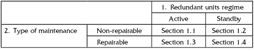
In accordance with such very rough classifications of redundancy methods, this chapter structure will be arranged as presented in Table 1.1.
TABLE 1.1 Types of Redundancy
We consider two main reliability indices: probability of failure-free operation during some required fixed time t0, R(t0), and mean time to failure, T. In practice, we often deal with a system consisting of a serial connection of redundant groups (see Fig. 1.1). Usually, such kinds of structures are found in systems with spare stocks with periodical replenishment.
FIGURE 1.1 General block diagram of series connection of redundant groups.

1.2 Non-repairable Redundant Group with Active Redundant Units
Let us begin with a simplest redundant group of two units (duplication), as in Figure 1.2.
FIGURE 1.2 Block diagram of a duplicated system.

Such a system operates successfully if at least one unit is operating. If one denotes random time to failure of unit k by ξk, then the system time to failure, ξ, could be written as
The time diagram in Figure 1.3 explains Equation (1.1).
FIGURE 1.3 Time diagram for a non-repairable duplicated system with both units active.

The probability of failure-free operation (PFFO) during time t for this system is equal to
(1.2) ![]()
where r(t) is PFFO of a single active unit.
We will assume an exponential distribution of time to failure for an active unit:
(1.3) ![]()
In this case the mean time to failure (MTTF), T, is equal to:
(1.4) 
Now consider a group of n redundant units that survives if at least one unit is operating (Fig. 1.4).
FIGURE 1.4 Block diagram of redundant group of n active units.

We omit further detailed explanations that could be found in any textbook on reliability (see Bibliography to Chapter 1).
For this case PFFO is equal:
(1.5) ![]()
and the mean time to failure (under assumption of the exponential failure distribution) is
(1.6) 
The most practical system of interest is the so-called k out of n structure. In this case, the system consists of n active units in total. The system is deemed to be operating successfully if k or more units have not failed (sometimes this type of redundancy is called “floating”). The simplest system frequently found in engineering practice is a “2 out of 3” structure (see Fig. 1.5).
FIGURE 1.5 Block diagram of a “2 out of 3” structure with active redundant unit.

A block diagram for general case can be presented in the following conditional way. It is assumed that any redundant unit can immediately operate instead of any of k “main” units in case a failure.
FIGURE 1.6 Block diagram of a “k out of n” structure with active redundant units.
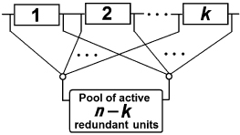
Redundancy of this type can be found in multi-channel systems, for instance, in base stations of various telecommunication networks: transmitter or receiver modules form a redundant group that includes operating units as well as a pool of active redundant units.
Such a system is operating until at least k of its units are operating (i.e., less than n − k + 1 failures have occurred). Thus, PFFO in this case is

and
(1.8) 
If a system is highly reliable, sometimes it is more reasonable to use Equation (1.7) in supplementary form (especially for approximate calculations when p(t) is close to 1).
(1.9) 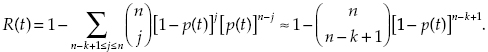
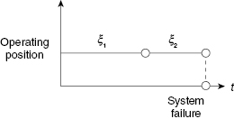
1.3 Non-repairable Redundant Group with Standby Redundant Units
Again, begin with a duplicated system presented in Figure 1.7. For this type of system, the random time to failure is equal to:
FIGURE 1.7 A non-repairable duplicated system with a standby redundant unit. (Here gray color denotes a standby unit.)

The time diagram in Figure 1.8 explains Equation (1.10). The PFFO of a considered duplicate system can be written in the form:
(1.11) ![]()
FIGURE 1.8 Time diagram for a non-repairable duplicated system with a standby redundant unit.
where p0(t) is the probability of no failures at time interval [0, t], and p1(t) is the probability of exactly one failure in the same time interval. Under assumption of exponentiality of the time-to-failure distribution, one can write:
(1.12) ![]()
and
(1.13) ![]()
so finally
(1.14) ![]()
Mean time to failure is defined as
(1.15) ![]()
since λ = 1/T.
For a multiple standby redundancy, a block diagram can be presented in the form shown in Figure 1.9. For this redundant group, one can easily write (using the arguments given above):
(1.16) 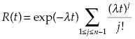
and
(1.17) ![]()
FIGURE 1.9 Block diagram of redundant group of one active and n − 1 standby units. (Here gray boxes indicate standby units.)

A block diagram for a general case of standby redundancy of k out of n type can be presented as shown in Figure 1.10. It is assumed that any failed operational unit can be instantaneously replaced by a spare unit. Of course, no replacement can be done instantaneously: in these cases, we keep in mind the five-second rule.1
FIGURE 1.10 Block diagram of a “k out of n” structure with standby redundant units. (Here gray color is used to show standby redundant units.)

This type of redundant group can be found in spare inventory with periodical restocking. Such replenishment is typical, for instance, for terrestrially distributed base stations of global satellite telecommunication systems. One observes a Poisson process of operating unit failures with parameter kλ, and the group operates until the number of failures exceeds n − k. The system PFFO during time t is equal to:
(1.18) 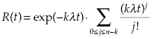
and the system MTTF is
(1.19) ![]()
Of course, there are more complex structures that involve active and standby redundant units within the same redundant group. For instance, structure “k out of n” with active units could have additional “cold” redundancy that allows performing “painless” replacements of failed units.
1.4 Repairable Redundant Group with Active Redundant Units
Consider a group of two active redundant units, that is, two units in parallel. Each unit operates independently: after failure it is repaired during some time and then returns to its position. Behavior of each unit can be described as an alternating stochastic process: a unit changes its states: one of proper functionality during time ξ, followed by a failure state induced repair interval, η. The cycle of working/repairing repeats. This process is illustrated in Figure 1.11. From the figure, one can see that system failure occurs when failure intervals of both units overlap.
FIGURE 1.11 Time diagram for a repairable system with standby redundancy. White parts of a strip denote operating state of a unit and black parts its failure state. Here ![]() denotes jth operating interval of unit i, and
denotes jth operating interval of unit i, and ![]() denotes jth interval of repair of this unit.
denotes jth interval of repair of this unit.
Notice that for repairable systems, one of the most significant reliability indices is the so-called availability coefficient, ![]() . This reliability index is defined as the probability that the system is in a working state at some arbitrary moment of time. (This moment of time is assumed to be “far enough” from the moment the process starts.) It is clear that this probability for a single unit is equal to a portion of total time when a unit is in a working state, that is,
. This reliability index is defined as the probability that the system is in a working state at some arbitrary moment of time. (This moment of time is assumed to be “far enough” from the moment the process starts.) It is clear that this probability for a single unit is equal to a portion of total time when a unit is in a working state, that is,
(1.20) ![]()
If there are no restrictions, that is, each unit can be repaired independently, the system availability coefficient, ![]() , can be written easily:
, can be written easily:
(1.21) ![]()
For general types of distributions, reliability analysis is not simple. However, if one assumes exponential distributions for both ξ and η, reliability analysis can be performed with the help of Markov models.
If a redundant group consists of two units, there are two possible regimes of repair, depending on the number of repair facilities. If there is a single repair facility, units become dependent through the repair process: the failed unit can find the facility busy with the repair of a previously failed unit. Otherwise, units operate independently. Markov transition graphs for both cases are presented in Figure 1.12.
FIGURE 1.12 Transition graphs for repairable duplicated system with active redundancy for two cases: restricted repair (only one failed unit can be repaired at a time) and unrestricted repair (each failed unit can be repaired independently). The digit in the circle denotes the number of failed units.

With the help of these transition graphs, one can easily write down a system of linear differential equations that can be used for obtaining various reliability indices. Take any two of the three equations:
(1.22) 
and take into account chosen initial conditions.
The availability coefficient for these two cases can be calculated using the formulas (where γ = λ/μ) in Table 1.2. However, our intent is to present methods of optimal redundancy rather than to give detailed analysis of redundant systems. (Such analysis can be found almost in any book listed in the Bibliography to Chapter 1.) Thus we will consider only the simplest models of redundant systems, that is, systems with unrestricted repair.
TABLE 1.2 Availability Coefficient for Two Repair Regimes
| Formula for availability coefficient, | ||
|---|---|---|
| Restricted repair | Unrestricted repair | |
| Strict formula | ||
| Approximation for γ << 1 | 1 − γ2 | 1 − 2γ2 |
We avoid strict formulas because they are extremely clumsy; instead we present only approximate ones that mostly are used in practical engineering calculations (Table 1.3).
TABLE 1.3 Approximate Formulas for Availability Coefficient
| Type of redundant group | Approximate formula for availability coefficient, | |
|---|---|---|
| Restricted repair | Unrestricted repair | |
| Group of n units | 1 − (n!)·γn | 1 − γn |
| Group of type “k out of n” | ||
1.5 Repairable Redundant Group with Standby Redundant Units
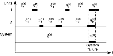
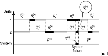
Consider now a repairable group of two units: one active and one standby. Behavior of such a redundant group can be described with the help of a renewal process: after a failure of the operating unit a standby unit becomes the newly operating one, while the failed unit after repair becomes a standby one, and so on. System failure occurs when a unit undergoing repair is not ready to replace a now not operating unit that has just failed. The process of functioning in this type of duplicated system is illustrated in Figure 1.13. In this case, finding PFFO of the duplicated system is also possible with the use of Markov models under assumption of exponentiality of both distributions (of repair time and time to failure).
FIGURE 1.13 Time diagram for a repairable duplicated system with standby redundancy. White parts of a strip denote the operating state of a unit, gray parts show the standby state, and black parts show the failure state. Here ![]() denotes jth operating interval of unit i, and
denotes jth operating interval of unit i, and ![]() denotes jth interval of repair of this unit.
denotes jth interval of repair of this unit.
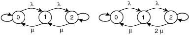
Transition graphs for restricted and unrestricted repair are shown in Figure 1.14.
FIGURE 1.14 Transition graphs for repairable duplicated systems with standby redundancy for two cases: restricted repair (only one failed unit can be repaired at a time) and unrestricted repair (each failed unit can be repaired independently).
Again, we present only approximate formulas in Table 1.4.
TABLE 1.4 Approximate Formulas for Availability Coefficient
| Type of redundant group | Approximate formula for availability coefficient, | |
|---|---|---|
| Restricted repair | Unrestricted repair | |
| Group of n units | ||
| Group of type “k out of n” | ||
1.6 Multi-level Systems and System Performance Estimation
Operation of a complex multi-level system cannot be satisfactorily described in traditional reliability terms. In this case, one has to talk about performance level of such systems rather than simple binary type “up and down” operating.
Let a system consist of n independent units characterized by their reliability indices p1, p2, …, pn. Assume that with unit failure a level of system performance degrades. Denote by Φi a quantitative measure of the system performance under the condition that unit i failed, by Φij the same measure if units i and j failed, and in general, if some set of units, α have failed then the system performance is characterized by value Φa. In this case the system performance can be characterized by the mean value:
(1.23) ![]()
where A is a set of all possible states of units 1, 2, …, n, that is, power of this set is 2n and
(1.24) ![]()
where notation A α means the total set of unit subscripts with exclusion of subset α.
The measure of system performance could be taken from conditional probability of successful fulfillment of the operation, productivity, or other operational parameters.
Several years after Kozlov and Ushakov (1966) had been published, there was a relative silence with quite rare appearance of works on the topic. Since average measure is not always a good characterization, soon there was a suggestion to evaluate the probability that multi-state system performance is exceeding some required level. In a sense, it was nothing more than introducing a failure criterion for a multi-state system. In this case, new formulation of the system reliability has the form
(1.25) ![]()
In 1985, Kurt Reinschke (in Ushakov, 1985) introduced a system that itself consists of multi-state units. However, this work also did not find an appropriate response among reliability specialists at the time.
Nevertheless, reliability analysis of multi-state systems has started for all three possible classes:
In the late 1990s, there was a veritable avalanche of papers on this topic, which has maintained a steady flow ever since. This subject is considered in more detail in Chapter 11.
Naturally, after multi-system analysis, attention to the problems of optimal redundancy in such systems arose. Now the problem of optimal redundancy in multi-state systems is a subject of intensive research.
1.7 Brief Review of Other Types of Redundancy
In reliability theory, redundancy is understood as using additional units for replacement/substitution of failed units. Actually, there are many various types of redundancy. Below we briefly consider structural redundancy, functional redundancy, a system with spare time for operation performance, and so on.
1.7.1 Two-Pole Structures
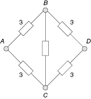
One of the typical types of structural redundancy is presented by networks. The simplest network structure is the so-called bridge structure (see Fig. 1.15). Assume that a connection between points A and D is needed.
FIGURE 1.15 Bridge structure.

A failure of any one unit does not lead to failure of the system because of the redundant structure. There are the following paths from A to D: ABD, ACD, ACBD, and ABCD. If at least one of those paths exists, the system performs its task. Of course, one can consider all cuts that lead to the system failure: AB&AC, BD&CD, AB&BC&CD, and AC&BC&BD. However, in this case we cannot use simple formulas of series and parallel systems, since paths are interdependent, as are cuts. Because of this, one can only write the upper and lower bounds for PFFO of such systems:
(1.26) 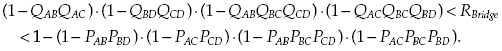
For this simple case, one can find a strict solution using a straightforward enumeration of all possible system states:
(1.27) ![]()
More complex systems of this type are presented by the two-pole networks: in such systems a “signal” has to be delivered from terminal A to terminal B (see Fig. 1.16). Reliability analysis of such systems is normally performed with the use of Monte Carlo simulation.
FIGURE 1.16 An example of a two-pole network.

For networks with a general structure, the exact value of the reliability index can be found only with the help of a direct enumeration. For evaluation of this index, one can use the upper and lower bounds of two types: Esary-Proschan boundaries (Barlow and Proschan, 1965) or Litvak-Ushakov boundaries (Ushakov, ed., 1985). Unfortunately, boundaries cannot be effectively used for solving optimal redundancy problems.
1.7.2 Multi-Pole Networks
This kind of network is very common in modern life, appearing in telecommunication networks, transportation and energy grids, and so on. The most important specific of such systems is their structural redundancy and the redundant capacity of their components. We demonstrate the specifics of such systems using a simple illustrative example. Consider the bridge structure that was described above, but assume that each node is either a “sender” or a “receiver” of “flows” to each other. Of course, flows can be different, as well as the capacities of particular links. Assume that traffic is symmetrical, that is, traffic from X to Y is equal to traffic from Y to X. This assumption allows us to consider only one-way flow between any points.
Let the traffic in the considered network be described as is shown in Table 1.5. For normal operating, it is enough to have the capacities of the links as described in Figure 1.17. (We will assume that traffic within the network is distributed as uniformly as possible.)
TABLE 1.5 Traffic in the Network (in conditional units)
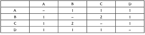
FIGURE 1.17 Traffic distribution.

However, links (as well as nodes) are subject to failure. For protection of the system against link failures, let us consider possible scenarios of link failure and measures of system protection by means of links' capacities increase.
What should we do if link AB has failed? The flow from A to B and from A to D should be redirected. Thus, successful operation of the network requires an increase of the links' capacities (see Fig. 1.18).
FIGURE 1.18 Traffic distribution in the case of link AB failure.

Since all four outside links are similar, failure of any link (AC, BD, or CD) leads to a similar situation. Thus, to protect the system against failure of any outside link, one should increase the capacities of each outside link from 2 to 3 units.
What happens if link BC fails? This link originally was used only for connecting nodes B and C. This traffic should be redistributed: half of the flow is directed through links BA–AC, and the rest through links BD–DC. To protect the system against link BC failure, the capacity of each outside link has to be increased by one unit.
FIGURE 1.19 Traffic distribution in the case of link BC failure.
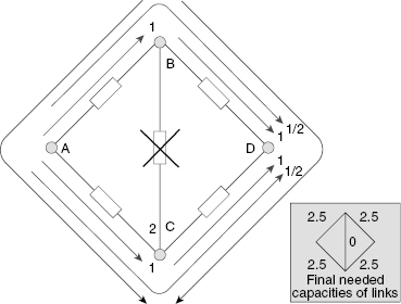
To protect the system against any single link failure, one has to make link capacities corresponding to the maximum at each considered scenario, as demonstrated in Figure 1.20.
FIGURE 1.20 Final values of link capacities for a network protected against any possible single failure.
1.7.3 Branching Structures
Another rather specific type of redundant system is a branching structure system (see Fig. 1.21). In such systems, actual operational units are on the lowest level, and successfully operate only under the condition that their controlling units at the upper levels are successfully operating. Such structures are very common, especially in military control systems.
FIGURE 1.21 System with branching structure.

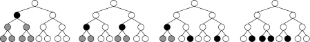
Assume that the branching system performs satisfactorily until four or more units of the lower level failed or lost control by upper level units. Types of possible system failures are given in Figure 1.22.
FIGURE 1.22 Types of situations when the branching system has 4 lower level units that have failed to perform needed operations. (Failed units are in black and units without control are in gray.)
Of course, for complex systems the concept of “failure” is not adequate; instead, there is the notion of diminished performance. For instance, for the same branching system considered above, it is possible to introduce several levels of performance. Assume that the system performance depending on the system state is described by Table 1.6.
TABLE 1.6 Levels of System Performance for Various System States
| Quantity of failed units of lower level | Conditional level of performance |
|---|---|
| 0 | 100% |
| 1 | 99% |
| 2 | 95% |
| 3 | 80% |
| 4 | 60% |
| 5 | 50% |
| 6 | 10% |
| 7 | 2% |
| 8 | 0% |
Usually, for such systems with structural redundancy, one uses the average level of performance. However, it is possible to introduce a new failure criterion and talk about the reliability of such a system. For instance, under the assumption that admissible level of performance is 80%, one comes to the situation considered above: the system is considered failed only when four (or more) of its lower level units do not operate sufficiently (failed or lost control).
1.7.4 Functional Redundancy
Sometimes to increase the probability of successful performance of a system, designers envisage functional redundancy, that is, make it possible to use several different ways of completing a mission. As an example, one can consider the procedure of docking a space shuttle with a space station (Fig. 1.23).
FIGURE 1.23 Phases of a space shuttle docking to a space station.

This complex procedure can be fulfilled with the use of several various methods: by signals from the ground Mission Control Center (MCC), by the on-board computer system, and manually. In all these cases, video images sent from space objects are usually used. However, MCC can also use telemetry data. All methods can ensure success of the operation, though with different performance.
1.8 Time Redundancy
One very specific type of redundancy is the so-called time redundancy. There are three main schemes of time redundancy.
Denote the probability of success for such a system by R(t0 | τ). If there is a failure on interval [0, t0] at such moment x < τ that still t0 − x > τ, the needed operation can be restarted, otherwise R(t0 | τ) = 0. This verbal explanation leads us to the recurrent expression
(1.28) 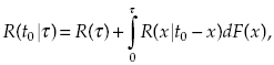
where F(x) is distribution function of the system time to failure.
These types of recurrent equations are usually solved numerically.
Denote the distribution of repair time, η, by G(t). If the first failure has occurred at moment x such that x > θ, it means that the system fulfilled its operation. If failure happens at moment ξ, the system can continue its operation after repair that takes time η, only if t0 − η > θ. It is clear that the probability that the total operating time during interval [0, t0] is no less than θ is equal to the probability that the total repair time during the same interval is no larger than t0 − θ.
For this probability, one considers two events that lead to success:
- System works without failures during time θ from the beginning.
- System has failed at the moment x < t0 − θ, and was repaired during time y, and during the remaining interval of t0 − x − y accumulates θ − x units of time of successful operation. This verbal description permits us to write the following recurrent expression:
(1.29)
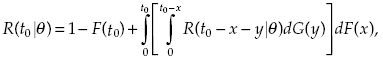
where R(t0 | z) = 0 if z < θ.
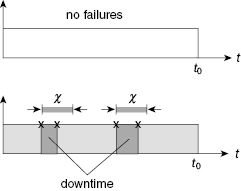
A system is considered to be successfully operating if during period [0, t0] there is no down time longer than ψ. This case, in some sense, is a “mirror” of what was considered at the beginning. We will skip explanation details and immediately write the recurrent expression:
(1.30) 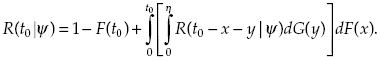
We will not consider this type of redundancy in details; instead we refer the reader to special literature on the subject (Cherkesov, 1974; Kredentser, 1978).
FIGURE 1.24 Examples of possible implementation of the successful system operation.

FIGURE 1.25 Examples of possible implementation of the successful system operation.

FIGURE 1.26 Time diagram for a system accumulating operation time.
1.9 Some Additional Optimization Problems
1.9.1 Dynamic Redundancy
Dynamic redundancy models occupy an intermediate place between optimal redundancy and inventory control models.
The essence of a dynamic redundancy problem is contained in the following. Consider a system with n redundant units. Some redundant units are operating and represent an active redundancy. These units can be instantly switched into a working position without delay and, consequently, do not interrupt the normal operation of the system. These units have the same reliability parameters (e.g., for exponential distribution, and the same failure rate). The remaining units are on standby and cannot fail while waiting. But at the same time, these units can be switched in an active redundant regime only at some predetermined moments of time. The total number of such switching moments is usually restricted because of different technical and/or economical reasons.
A system failure occurs when at some moment there are no active redundant units to replace the main ones that have failed. At the same time, there may be many standby units that cannot be used because they cannot be instantly switched after a system failure.
Such situations in practice can arise in different space vehicles that are participating in long journeys through the Solar System. A similar situation occurs when one considers using uncontrolled remote technical objects whose monitoring and service can be performed only rarely.
It is clear that if all redundant units are switched to an active working position at an initial moment t = 0, the expenditure of these units is highest. Indeed, many units might fail in vain during the initial period. At the same time, the probability of the unit's failure during this interval will be small. On the other hand, if there are few active redundant units operating in the interval between two neighboring switching points, the probability of the system's failure decreases. In other words, from a general viewpoint, there should exist an optimal rule (program) of switching standby units into an active regime and allocating these units over all these periods.
Before we begin to formulate the mathematical problem, we discuss some important features of this problem in general.
Goal Function
Two main reliability indices are usually analyzed: the probability of failure-free system operation during some specified interval of time, and the mean time to system failure.
System Structure
Usually, for this type of problem, a parallel system is under analytical consideration. Even a simple series system requires a very complex analysis.
Using Active Redundant Units
One possibility is that actively redundant units might be used only during one period after being switched into the system. Afterward, they are no longer used, even if they have not failed. In other words, all units are divided in advance into several independent groups, and each group is working during its own specified period of time. After this period has ended, another group is switched into the active regime. In some sense, this regime is similar to the preventive maintenance regime.
Another possibility is to keep operationally redundant units in use for the next stages of operation. This is more effective but may entail some technical difficulties.
Controlled Parameters
As we mentioned above, there are two main parameters under our control: the moments of switching (i.e., the periods of work) and the number of units switched at each switching moment. Three particular problems arise: we need to choose the switching moments if the numbers of switched units are fixed in each stage; we need to choose the numbers of units switched in each stage if the switching moments are specified in advance; and, in general, we need to choose both the switching moments and the numbers of units switched at each stage.
Classes of Control
Consider two main classes of switching control. The first one is the so-called prior rule (program switching) where all decisions are made in advance at time t = 0. The second class is the dynamic rule where a decision about switching is made on the basis of current information about a system's state (number of forthcoming stages, number of standby units, number of operationally active units at the moment, etc.).
We note that analytical solutions are possible only for exponentially distributed TTFs. The only possible method of analysis for an arbitrary distribution is via a Monte Carlo simulation.
Note
1 Russian joke: If a fallen object is picked up in 5 seconds, it is assumed that it hasn't fallen at all.
Chronological Bibliography of Main Monographs on Reliability Theory (with topics on Optimization)
Lloyd, D.K., and Lipov, M. 1962. Reliaility Management, Methods and Mathematics. Prentice Hall.
Barlow, R.E., and F. Proschan. 1965. Mathematical Theory of Reliability. John Wiley & Sons.
Kozlov, B.A., and Ushakov, I.A. 1966. Brief Handbook on Reliability of Electronic Devices. Sovetskoe Radio.
Raikin, A.L. 1967. Elements of Reliability Theory for Engineering Design. Sovetskoe Radio.
Polovko, A.M. 1968. Fundamentals of Reliability Theory. Academic Press.
Gnedenko, B.V., Belyaev, Y.K., and Solovyev, A.D. 1969. Mathematical Methods in Reliability Theory. Academic Press.
Ushakov, I.A. 1969. Method of Solving Optimal Redundancy Problems under Constraints (in Russian). Sovetskoe Radio.
Kozlov, B.A., and Ushakov, I.A. 1970. Reliability Handbook. Holt, Rinehart & Winston.
Cherkesov, G.N. 1974. Reliability of Technical Systems with Time Redundancy (in Russian). Sovetskoe Radio.
Barlow, R.E., and Proschan, F. 1975. Statistical Theory of Reliability and Life Testing. Holt, Rinehart & Winston.
Gadasin, V.A., and Ushakov, I.A. 1975. Reliability of Complex Information and Control Systems (in Russian). Sovetskoe Radio.
Kozlov, B.A., and Ushakov, I.A. 1975. Handbook of Reliability Calculations for Electronic and Automatic Equipment (in Russian). Sovetskoe Radio.
Kozlow, B.A., and Uschakow, I.A. 1978. Handbuch zur Berehnung der Zuverlassigkeit in Elektronik und Automatechnik (in German). Academie-Verlag.
Kredentser, B.P. 1978. Forcasting Reliability for Time Redundamcy (in Russian). Naukova Dumka.
Raikin, A.L. 1978. Reliability Theory of Complex Systems (in Russian). Sovietskoe Radio.
Kozlow, B.A., and Uschakow, I.A. 1979. Handbuch zur Berehnung der Zuverlassigkeit in Elektronik und Automatechnik (in German). Springer-Verlag.
Tillman, F.A., Hwang, C.L., and Kuo, W. 1980. Optimization of System Reliability. Marcel Dekker.
Barlow, R.E., and Proschan, F. 1981. Statistical Theory of Reliability and Life Testing, 2nd ed.
Gnedenko, B.V., ed. 1983. Aspects of Mathematical Theory of Reliability (in Russian). Radio i Svyaz.
Ushakov, I.A. 1983. Textbook on Reliability Engineering (in Bulgarian). VMEI.
Ushakov, I.A., ed. 1985. Handbook on Reliability (in Russian). Radio i Svyaz.
Rudenko, Y.N., and Ushakov, I.A. 1986. Reliability of Power Systems (in Russian). Nauka.
Reinschke, K., and Ushakov, I.A. 1987. Application of Graph Theory for Reliability Analysis (in German). Verlag Technik.
Reinschke, K., and Ushakov, I.A. 1988. Application of Graph Theory for Reliability Analysis (in Russian). Radio i Svyaz.
Reinschke, K., and Ushakov, I.A. 1988. Application of Graph Theory for Reliability Analysis (in German). Springer, Munchen-Vien.
Rudenko, Y.N., and Ushakov, I.A. 1989. Reliability of Power Systems, 2nd ed. (in Russian). Nauka.
Kececioglu, D. 1991. Reliability Engineering Handbook. Prentice-Hall.
Volkovich, V.L., Voloshin, A.F., Ushakov, I.A., and Zaslavsky, V.A. 1992. Models and Methods of Optimization of Complex Systems Reliability (in Russian). Naukova Dumka.
Ushakov, I.A. 1994. Handbook of Reliability Engineering. John Wiley & Sons.
Gnedenko, B.V., and Ushakov, I.A. 1995. Probabilistic Reliability Engineering. John Wiley & Sons.
Kapur, K.C., and Lamberson, L.R. 1997. Reliability in Engineering Design. John Wiley & Sons.
Gnedenko, B.V., Pavlov, I.V., and Ushakov, I.A. 1999. Statistical Reliability Engineering. John Wiley & Sons.
Kuo, W., and Zuo, M.J. 2003. Optimal Reliability Modeling: Principles and Applications. John Wiley & Sons.
Pham, H. 2003. Handbook of Reliability Engineering. Springer.
Kuo, W., Prasad, V.R., Tillman, F.A., and Hwang, C.-L. 2006. Optimal Reliability Design: Fundamentals and Applications. Cambridge University Press.
Levitin, G., ed. 2006. Computational Intelligence in Reliability Engineering. Evolutionary Techniques in Reliability Analysis and Optimization. Series: Studies in Computational Intelligence, vol. 39. Springer-Verlag.
Ushakov, I.A. 2007. Course on Reliability Theory (in Russian). Drofa.
Gertsbakh, I., and Shpungin, Y. 2010. Models of Network Reliability. CRC Press.