4.1 The Main Idea of SDM

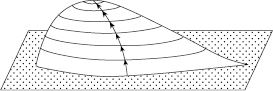
The Steepest Descent Method (SDM) is based on a very natural idea: moving from an arbitrary point in the direction of the maximal gradient of the goal function, it is possible to reach the maximum of a multi-dimensional unimodal function. The origin of the method's name lies in the fact that a water drop runs down a non-flat surface choosing the direction of instantaneous maximum descent.

The next simple example explains the algorithm more graphically. Suppose that a traveler comes to a hill that is hidden in a thick mist. His goal is to reach the hill top with no knowledge about the mountain shape except the fact that the hill is smooth enough (has no ravines or local hills). The traveler sees only a very restricted area around the starting point. The question is: What is the shortest path from the initial point to the mountain's top? Intuition hints that the traveler has to move in the direction of the maximal possible ascent at each point on his path to the mountain's top (Fig. 4.1). This direction coincides with the gradient of the function at each point.

FIGURE 4.1 A path of a traveler up to the hill top.

However, optimal redundancy problems have an integer nature: redundant units can be added to the system one by one. The previous analogy is useful in case of continuous functions of continuous arguments. But in the case of optimal redundancy, all arguments are discrete. If we continue the analogy with the traveler, one sees that there are restrictions on the traveler's movement: he can move only in the north–south or east–west directions and can change the direction only at the vertices of a discrete grid with specified steps (Fig. 4.2). This means that at each vertex one should use the direction of the largest partial derivative. Because of this, one sometimes speaks of the Method of Coordinate Steepest Descent.

FIGURE 4.2 A traveler's path when only north–south and east–west directions are allowed.

This idea of finding the maximum of a unimodal function may be applied to the optimal redundancy problem.

4.2 Description of the Algorithm

Consider a system that is a series connection of independent redundant groups. Let us use the both goal functions in the additive form

(4.1)

and

(4.2)

It is clear that maximization of function R(X) corresponds to minimization of function L(X), that is, the optimum solution X^opt for goal function L(X) delivers as well the optimum for function R(X).

Introduce vector , where is the number of redundant units of the ith redundant group at the nth step of the SDM process. Denote by the reliability index and by the cost of the ith redundant group after the nth step of the SDM process. For the convenience of further exposition, let us also introduce the following additional notation: , that is, vector is vector X without component x_i. Obviously, .

At the nth step of the process, one adds a redundant unit of type k, for which the relative increase of reliability index is at the maximum, that is,

(4.3)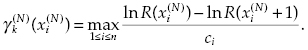

A unit of this type is added to the set of the system's redundant units. The process continues in the same manner until the optimal solution is obtained.

Now let us describe the optimization algorithm step by step from the very beginning.

1. Before the beginning of the process, there are no redundant units at all, that is, or, in other words, .

2. For all i, i=1, 2, …, n, one calculates values .

3. One finds such index k that delivers maximum

4. One calculates a new value

5. All other , i ≠ k, change their superscripts: .

6. One gets a new vector of the system's redundant units:

7. One calculates the value of L(X⁽¹⁾) and determines the corresponding R(X⁽¹⁾).

8. One calculates the value of L(X⁽¹⁾).

9. One calculates by the same rule a new value .

10. All other values , i ≠ k, are conserved but one changes their superscripts:

11. GOTO (3).

4.3 The Stopping Rule

The solution of the direct problem of optimal redundancy is reached at such step N for which the following condition is valid:

(4.4)

The value of R(X^(N)) is the maximum possible for the given constrain on the system cost.

Sometimes the SDM procedure requires one to add at the last step a very expensive unit but adding this unit exceeds the given constraint on the total cost of the system's redundant units. At the same time, if one does not add this unit, there are some extra financial resources to add other, less expensive units. In this case one may bypass the expensive unit and continue the procedure.

The inverse optimal redundancy problem reaches its optimal solution at step N where the following condition is valid:

(4.5)

The value of C(X^(N)) is the minimum possible for the given constraint on the required system reliability index.

American mathematician Frank Proschan (Barlow and Proschan, 1965, 1981; see Box) has proven that the SDM procedure delivers members of dominating sequences if each function R_i(x_i) is concave.

Frank Proschan (1921–1993)

Frank Proschan was an American mathematician who earned his Ph.D. in statistics from Stanford University in 1959. He had held positions with the Federal Government at the National Bureau of Standards (1941–1952), with Sylvania Electric Products (1952–1960), and with Boeing Scientific Labs (1960–1970). Beginning in 1970, he was Professor of Statistics at Florida State University. He won many honors including the Von Neumann Prize award presented by TIMS-ORSA. He was a Fellow of the Institute of the American Statistical Association and a member of the International Statistical Institute.

---

Example 4.1

A series system consists of six different units whose parameters are given in Table 4.1. (Distributions of time to failure are assumed exponential.)

TABLE 4.1 Units' Parameters

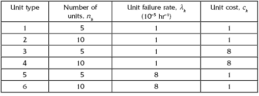
One needs to find the optimum number of standby units for successful system operation during t₀ = 1000 hours for two cases:

(1) Required probability of failure-free operation (PFFO) is 0.9995.

(2) Admissible expenses on all spare units are 40 cost units.

TABLE 4.2 Values of Parameters of Poisson Distribution

Parameter	Value
a1	1·10 −5·5·1000 = 0.05
a2	1·10 −5·10·1000 = 0.1
a3	1·10 −5·5·1000 = 0.05
a4	1·10 −5·10·1000 = 0.1
a5	8·10 −5·5·1000 = 0.4
a6	1·10 −5·10·1000 = 0.8

First, using Table 4.1, let us find parameters of Poisson distributions for each group by the formula a_i = λ_in_it₀. The probability of appearance of exactly k failures during given time t₀ is calculated by the formula:

(4.6)

By the way, if condition Q_i(x_i) >> Q_i(x_i + 1) holds, then calculation of values γ can be simplified up to

(4.7)

Calculated values of q_i(x_i) are presented in Table 4.3.

TABLE 4.3 Values of Unreliability Indices for Various x_i

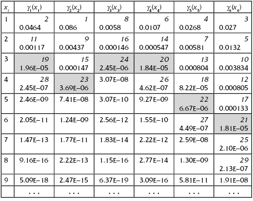
Now we can build Table 4.4, where values γ_i(x_i) are presented. In this table, the numbers in the upper right corner of cells are numbers corresponding to steps of the SDM procedure.

TABLE 4.4 Values γ_i(x_i) for All Redundant Groups

On the basis of Table 4.4, let us build the final table (Table 4.5), from which one can get needed optimal solutions. Table 4.5 allows finding optimal solutions for both optimal problems: direct as well as inverse.

TABLE 4.5 Step-by-Step Results of SDM Procedure

By conditions of the illustrative problem, R⁰ = 0.9995. From Table 4.5, we find that the solution is reached at step 18: unreliability in this case is 4.16E−04, that is, R(X^opt) = 0.999584 that satisfies the requirements. (Corresponding cost is 46 units.)

At the same time, for the inverse problem the solution is reached at step 15 with the total cost of 36 units. (Corresponding PFFO = 0.99669.) In this case we keep extra 4 cost units. Of course, they could be spent for 4 additional inexpensive units of types 1, 2, 5, and 6, that is, instead of the obtained solution (x₁ = 2, x₁ = 3, x₁ = 1, x₁ = 2, x₁ = 3, x₁ = 4), take solution with all resources spent: (x₁ = 3, x₁ = 4, x₁ = 1, x₁ = 2, x₁ = 4, x₁ = 5). In this case, the system PFFO is equal to 0.99844. This solution is admissible in sense of the total cost of redundant units.

By the way, to get such a solution we could slightly change the SDM algorithm: If on a current step of the SDM procedure we “jump” over the admissible cost, we can take another unit or units with admissible cost.

Analogous corrections could be performed if the obtained current solution for the direct problem of optimal redundancy overexceeds the required value R⁰.

---

4.5 Approximate Solution

For practical purposes, an engineer sometimes needs to know an approximate solution that would be close to an optimal one a priori. Such a solution can be used as the starting point for the SDM calculation procedure. (Moreover, sometimes the approximate solution is a good pragmatic solution if input statistical data are too vague. Indeed, attempts to use strong methods with unreliable input data might be considered lacking in common sense! Remember: the “garbage-in-garbage-out” rule is valid for precise mathematical models as well!)

The proposed approximate solution (Ushakov, 1965) is satisfactory for highly reliable systems. This means that in the direct optimal redundancy problem, the value of Q⁰ is very small. In a sense, such a condition is not a serious practical restriction. Indeed, if the investigated system is too unreliable, one should question if it is reasonable to improve its reliability at all. Maybe it is easier to find another solution using another system.

For a highly reliable system, one can write:

(4.8)

at the stopping moment (the nth step) of the optimization process, when the value of the reliability index should be high enough.

From Table 4.4, one can see that there is a “strip” that divides all values of γ_i(x_i). For instance, consider the cells corresponding to steps 19–24 (shadowed on the table). The largest value laying above this strip (step 18) has value γ = 8.22E−05, which is larger than any value of γ belonging to the strip. At the same time, the largest value laying below the strip (step 25) has value γ = 2·10⁻⁶, which is smaller than any corresponding value on the strip. This means that there is some value Λ, 2·10⁻⁶ < Λ < 8.22·10⁻⁵, that divides all sets of γ into two specific subsets: this Λ, in a sense, plays the role of a Lagrange multiplier. Indeed, the approximate equality of γ for each “argument” x_i completely corresponds to the equilibrium in the Lagrange solution.

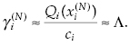
Let us make a reasonable assumption that at the stopping moment

(4.9)

At the same time,

(4.10)

Now using (4.8)

(4.11)

and finally

(4.12)

Now we can substitute Equation (4.12) into Equation (4.10) and obtain:

(4.13)

For solving the inverse optimal redundancy problem, one has to use a very simple iterative procedure.

(1) Find approximate starting values of the x_is

(4.14)

(2) Use these x_is to calculate Q⁽¹⁾ as

(4.15)

(3) Calculate g⁽¹⁾ as

(4.16)

(4) For γ⁽¹⁾ determine for all i from the equations

(4.17)

(5) For all obtained , one calculates the total cost of the system's redundant units as:

(4.18)

If C⁽¹⁾ > C⁰, one sets a new γ⁽²⁾ > γ⁽¹⁾; if C⁽¹⁾ < C⁰, one sets a new γ⁽²⁾ > γ⁽¹⁾.

After this, the procedure continues from the third step. Such an iterative procedure continues until the appropriate value of the total cost of redundant units is achieved.

Chronological Bibliography

Barlow, R. E., and Proschan, F. 1965. Mathematical Theory of Reliability. John Wiley & Sons.

Ushakov, I. A. 1965. “Approximate solution of optimal redundancy problem.” Radiotechnika, no. 12.

Ushakov, I. A. 1967. “On optimal redundancy problems with a non-multiplicative objective function.” Automation and Remote Control, no. 3.

Ushakov, I. A. 1969. Method of Solving Optimal Redundancy Problems under Constraints (in Russian). Sovetskoe Radio.

Ushakov, I. A. 1981. “Methods of Approximate Solution of Dynamic Standby Problems.” Engineering Cybernetics, vol. 19, no. 2.