10.1 Method of “Weighing Costs”

A number of cases arise where one has to take into account several restrictions in solving the optimal redundancy problem. For example, various objects such as aircraft, satellites, and submarines have restrictions on cost and also on weight, volume, required electric power, and so on. (Apparently, the cost for most of these technical objects is an important factor, but, perhaps, less important than others mentioned.)

In these cases, one has to solve the optimization problem under several restrictions and to maximize the system reliability index under restrictions on all other factors.

Consider a system consisting of n redundant groups connected in series. For each additional redundant unit of the system, one has to spend some quantity of M various types of resources (for instance, cost, weight, or volume), say, C_j(X). There are constraints on each type of resource: . The optimization problem is formulated as:

(10.1)

where X = (x₁, x₂, … , x_n) is the vector of the system redundant units.

Let us assume that each C_j(X) is a linear function of the form

(10.2)

where c_ji is the resource of type j associated with a unit of type i.

One of the most convenient ways to solve this problem is reducing it to a one-dimensional problem. To this end, we introduce “weight” coefficients d_j such that: 0 ≤ d_j ≤ 1, and

(10.3)

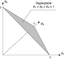
A set of d_j satisfying Equation (10.3) presents a diagonal hyperplane within n-dimensional unitary hypercube. Denote this hyperplane by D. An explanation is given for a three-dimensional case in Figure 10.1.

FIGURE 10.1 Hyperplane with all possible d_j.

Use the steepest descent method (SDM) for the solution. The process of a solution is as follows. Choose a point , D^k ∈ D. Produce for each unit j “weighed cost” corresponding to vector D^k:

(10.4)

Solve a one-dimensional problem while simultaneously controlling all M constraints. As soon as the optimization procedure has been stopped due to a possible violation of at least one of the constraints, the value of a reached level of R^k and realized vector X^k are memorized.

Then the next vector, say, D^j, is chosen and new values R^j and X^j are found. Compare admissible solutions and keep that with the largest value of R.

The procedure of the oriented choosing of D^k rather than direct enumerating can be organized: the procedure of the steepest descent could be used for this purpose.

Perhaps an even better procedure is as follows. At the stopping moment, pay attention to the type of constraint that is closest to violation. Sometimes it means that the process is “less optimal” relating to this type of resource. Increase a corresponding weight multiplier and repeat the process.

As in most practical cases, finding the appropriate choice of increment to change d is more of an art than a science.

Maximum found value R corresponds to the optimal solution X^opt.

An illustrative example might be useful to demonstrate this method.

Example 10.1

Consider a series system consisting of three units with the characteristics given in Table 10.1.

TABLE 10.1 Data for Example 10.1

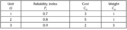
A “hot” redundancy is permitted to improve the system reliability. The problem is to find the optimal solutions for the following constraints on the redundant system units as a whole:

(1) Cost: conditional units; weight: conditional units.

(2) Cost: conditional units; weight: conditional units.

---

10.2 Method of Generalized Generating Functions

The problem treated above can be solved exactly with the use of the method of generalized generating functions. The legion for each ith redundant group is represented as the set of the cohorts

where N_i is the number of cohorts in this legion. (In principle, the number of cohorts is unrestricted in this investigation.) Each cohort consists of M + 2 maniples:

where M is the number of restrictions. All maniples are defined as in the one-dimensional case that we considered above. A similar interaction is performed with the maniples:

where J is the set of subscripts: J = (j₁, … , j_n).

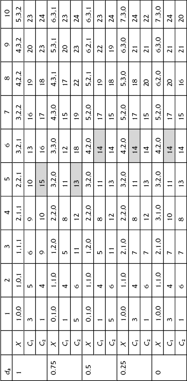
TABLE 10.2 Solution Process for Various d_j

The remaining formal procedures totally coincide with the one-dimensional case with one very important exception: instead of a scaler ordering, one must use the special ordering of the cohorts of the final legion.

It is difficult to demonstrate the procedure on a numerical example, so we give only a detailed verbal explanation.

Suppose we have the file of current cohorts ordered according to increasing R. If we have a specified set of restrictions: C_j(X) ≤ C_0j for all j: 1 ≤ j ≤ M, then there is no cohort in this file that violates at least one of these restrictions. When a new cohort, say, C_k, appears during the interaction procedure, it is put in the appropriate place in accordance with the value of its R-maniple. The computational problem is as follows.

After a multi-dimensional undominated sequence is constructed, one easily finds the solution for the multiple restrictions: it is the cohort with the largest R-maniple value (in other words, a cohort on the right if the set is ordered by the values of R).

The stopping rule for this procedure is to find the size of each cohort that will produce a large enough number of cohorts in the resulting legion so as to contain the optimal solution. At the same time, if the numbers of cohorts in the initial legions are too large, the computational procedure will take too much time and will demand too large a memory space.

Of course the simplicity of this description should not be deceptive. The problem is very bulky in the sense that the multi-dimensional restrictions and the large numbers of units in typical practical problems could require a huge memory and computational time. (But who can find a non-trivial multi-dimensional problem that has a simple solution?)

Chronological Bibliography

Proschan, F., and Bray, T. A. 1970. “Optimum redundancy under multiple constraints.” Operations Research, no. 13.

Ushakov, I. A. 1971. “Approximate solution of optimal redundancy problem for multipurpose system.” Soviet Journal of Computer and System Science, no. 2.

Ushakov, I. A. 1972. “A heuristic method of optimization of the redundancy of multipurpose system.” Soviet Journal of Computer and System Sciences, no. 4.

Nakagawa, Y., and. Miyazaki, S. 1981. “Surrogate constraints algorithm for reliability optimization problem with two constraints.” IEEE Transaction on Reliability, no. 30.

Genis, Y. G., and Ushakov, I. A. 1984. “Optimization of multi-purpose systems.” Soviet Journal of Computer and System Sciences, no. 3.