9.1 Comparison of Methods

Optimal redundancy is a very important practical problem. The solution of the problem allows one to improve reliability at a minimal expense. But here, as in many other practical problems, questions arise: What is the accuracy of the obtained results? What is the real effect of the use of sophisticated mathematics?

These are not unreasonable questions.

We have already discussed what it means to design an “accurate” mathematical model. It is always better to speak about a mathematical model which more or less correctly reflects a real object. But let us suppose that we are “almost sure” that the model is perfect. What price are we willing to pay for obtaining numerical results? What method is best, and best in what sense?

The use of excessively accurate methods is, for practical purposes, usually not necessary because of the uncertainty of the statistical data. On the other hand, it is inexcusable to use approximate methods without reason.

We compare the different methods in the sense of their accuracy and computation complication.

The Lagrange multiplier method (LMM) demands the availability of continuous, differentiable functions. This requirement is met very rarely: one usually deals with the essentially discrete nature of the resources. But LMM sometimes can be used for a rough estimation of the desired solution.

The steepest descent method (SDM) is very convenient from a computational viewpoint. It is reasonable to use this method if the resources that one might spend on redundancy are large. Of course, this generally coincides with the requirement of high system reliability because this usually involves large expenditures of resources. But unfortunately, it happens very rarely in practice. At any rate, one can use this approach for solution of most practical problems without hesitation.

The absolute difference between costs of the two neighboring SDM solutions cannot exceed the cost of the most expensive unit value. Thus, it is clear that the larger the total cost of the system, the smaller the relative error of the solution.

The dynamic programming method (DPM) and its modifications (Kettelle's Algorithm and the method of universal generating function) are exact, but they demand more calculation time and a larger computer memory. As with most discrete problems requiring an enumerating algorithm, these optimal redundancy problems are np-hard.

As we mentioned above, the SDM may even provide an absolutely exact solution, since a dominating sequence for SDM is a subset of dominating sequence of DPM. In Figure 9.1, one finds two solutions obtained by SDM and DPM. The black dots correspond to the sequence obtained by SDM, and the white dots correspond to DPM.

FIGURE 9.1 Comparison of DPM and SDM solutions.

Of course, one of the questions of interest is the stability of the solutions. How does the solution depend on the accuracy of the input data? How are the solutions obtained by the different methods distinguished? How much do the numerical results of the solutions differ from one method to another?

An illustration of the problem is given by numerical experiments.

Example 9.1

Consider a series system consisting of three units. The input data are assumed to be uncertain: units' probability of failure-free operation (PFFO) and cost are known with an accuracy of 10%. To demonstrate possible difference in solutions, let us take the five systems presented in Table 9.1.

TABLE 9.1 Five Different Systems Consisting of Similar Units with Slightly Different Values of Parameters

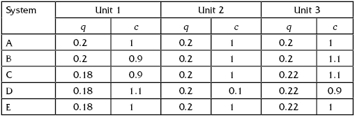
The problem is to check the stability of the optimal solutions over the range of variability of the parameters.

---

Solution to Example 9.1

At first, we compare the solutions for all five cases where the specified total system cost is to be at most 30 units. For each case, we give two results: one obtained by the SDM and the second (marked with *) obtained by the DPM. The results are presented in Table 9.2.

The table shows that the only differences between the approximate and exact solutions are observed for the cases C and C*. However, all solutions are very close.

With an increase in spent resources, the relative difference between the solutions obtained by the SDM and the DPM will be increasingly smaller.

We now analyze the solutions corresponding to a specified level of reliability. In Table 9.3, for the same systems, respective results for Q₀ = 1·10⁻⁶ are collected.

Numerical computer experiments and practical experience in solution of the optimal redundancy problem could aid in the development of a keen engineering intuition in the approximate solving of such problems and their sensitivity analysis.

TABLE 9.2 Optimal Numbers of Redundant Units for Five Systems Presented in Table 9.1 (the Level of Spent Resources Is under 30 Units)

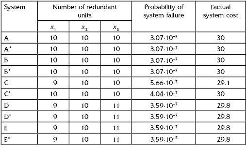
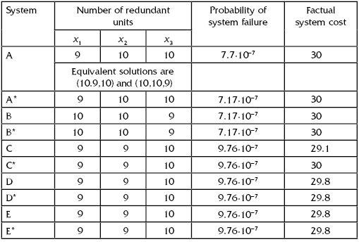
TABLE 9.3 Optimal Numbers of Redundant Units for Five Systems Presented in Table 9.1 (the Level of Required Reliability Is under 1·10 in Power)

---

9.2 Sensitivity Analysis of Optimal Redundancy Solutions

Solving practical optimal redundancy problems, one can ponder: what is the sense of optimizing if input data are plucked from the air? Indeed, statistical data are so unreliable (especially in reliability problems) that such doubts have a very good ground.

Not finding any sources after searching for the answer to this question, the author decided to make some investigation of optimal solution sensitivity under influence of data scattering.

A simple series system of six units has been considered (see Fig. 9.2). For reliability increase, one uses a loaded redundancy, that is, if a redundant group k has x_k redundant units, its reliability is

FIGURE 9.2 Series system that underwent analysis.

where p_k is the PFFO of a single unit k. The total cost of x_k redundant units is equal to c_k·x_k, where c_k is the cost of a single unit of type k.

Units' parameters are presented in Table 9.4.

TABLE 9.4 Input Data

Assume that units are mutually independent, that is, the system's reliability is defined as:

and the total system cost is:

Solutions of both problems of optimal redundancy are presented here:

direct:

and

inverse:

For finding the optimal solutions, the steepest descent method was applied. For this “base” system, the solutions for several sets of parameters are presented for the direct problem in Table 9.5 and for the inverse problem in Table 9.6. (Numbers are given with high accuracy only for demonstration purposes; in practice, one has to use only significant positions after a row of nines.)

TABLE 9.5 Solution for the Direct Problem

TABLE 9.6 Solution for the Inverse Problem

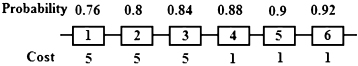
The question of interest is: How will the optimal solution change if input data are changed? Two types of experiments have been performed: in the first series of experiments, different units' costs with fixed probabilities were considered (see Fig. 9.3), and, in another one, different units' probabilities with fixed costs were considered (see Fig. 9.4).

FIGURE 9.3 Input data for the first series of experiments.

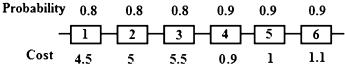
FIGURE 9.4 Input data for the second series of experiments.

The results of calculations are as shown in Table 9.7. In addition, a Monte Carlo simulation was performed where parameters of the PFFO and cost were changed simultaneously. In this case, parameters of each unit were calculated (in Excel) as:

TABLE 9.7 Values of Probabilities of Failure-Free Operations

and

that is, considered a random variation of the values within ±20% limits.

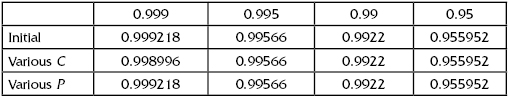
The final results for this case are presented in Table 9.8, Table 9.9, Table 9.10, and Table 9.11. Analysis of data presented in these tables shows relatively significant difference in numerical results (see Fig. 9.5). However, the problem is not in coincidence of final values of PFFO or cost. The problem is how the change of parameters influences the optimal values of x₁, x₂, ….

FIGURE 9.5 Deviation of maximum and minimum values of probability of failure-free operation obtained by Monte Carlo simulation.

TABLE 9.8 Results of Monte Carlo Simulations for P* = 0.999

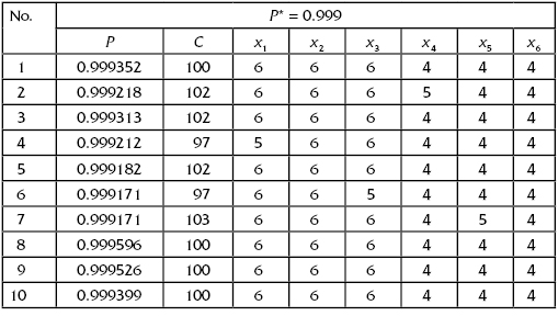
TABLE 9.9 Results of Monte Carlo Simulations for P* = 0.995

TABLE 9.10 Results of Monte Carlo Simulations for P* = 0.99

TABLE 9.11 Results of Monte Carlo Simulations for P* = 0.95

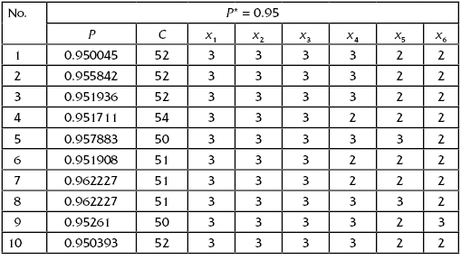
One can observe that even with a system of six units (redundant groups), a visual analysis of sets (x₁, x₂, … , x₆) is extremely difficult, and, at the same time, deductions based on some averages or deviations of various x_k are almost useless.

The author was forced to invent some kind of a special presentation of sets of x_ks. Since there is no official name for this kind of graphical presentation, it will be called a “multiple polygon.” On this type of multiple polygon, there are numbers of “rays” corresponding to the number of redundant of units (groups). Each ray has several levels corresponding to the number of calculated redundant units for the considered case (see Fig. 9.6).

FIGURE 9.6 Multiple polygon axes with numbered levels.

The multiple polygons give a perfect visualization of “close-to-optimal” solutions and characterize observed deviation of particular solutions. Such multiple polygons for considered example are given in Figure 9.7. (Here, bold lines are used for connecting the values of x_k obtained as optimal solution for units with parameters given in Table 9.4.)

FIGURE 9.7 Deviations of optimal solutions for randomly varied parameters from the optimal solution obtained for parameters given in Table 9.1.

Thus, one may notice that input parameter variation may influence significantly enough the probability of failure-free operation and the total system cost from run to run of Monte Carlo simulation, though the optimal solution remains more or less stable.