As mentioned earlier, the problem has an essentially discrete nature, so the SDM cannot guarantee the accuracy of the solution. Thus, if an exact solution of the optimal redundancy problem is needed, one generally needs to use the Dynamic Programming Method (DPM).

5.1 Bellman's Algorithm

The main ideas of the DPM were formulated by an American mathematician Richard Bellman (Bellman, 1957; see Box), who has formulated the so-called optimality principle.

Richard Ernest Bellman (1920–1984)

American applied mathematician, who is famous for his invention of dynamic programming in 1953. He also made many important contributions in other fields of mathematics. Over the course of his career Bellman published 619 papers and 39 books. During the last 11 years of his life he published over 100 papers, despite suffering from the crippling complications of brain surgery. Bellman's fundamental contributions to science and engineering won him many honors, including the First Norbert Wiener Prize in Applied Mathematics (1970).

---

The DPM provides an exact solution of discrete optimization problems. In fact, it is a well-organized method of direct enumeration. For the accuracy of the solutions, one has to pay with a high calculation time and a huge computer memory if the problem is highly dimensional.

To solve the direct optimal redundancy problem, let us construct a sequence of Bellman's function, B_k(r). This function reflects the optimal value of the goal function for a system of k redundant groups and a specified restriction r. As usual, we start at the beginning:

(5.1)

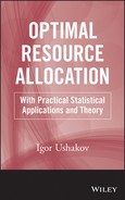
It is clear that in such a way we determine the number of units that are necessary for the redundant group to have a reliability index equal to r⁽¹⁾ that is within the interval [0, R⁰]. (See Fig. 5.1.)

FIGURE 5.1 Illustration of the solution for Equation (5.1).

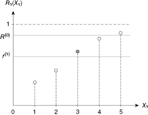
Now we compose the next function (see Fig. 5.2):

(5.2)

FIGURE 5.2 Illustration of the solution for Equation (5.2).

In a sense, we have a “convolution” of the first and second redundant groups, and for each level of current redundancy, the best variant of such convolution is kept for the next stage of the procedure. In an analogous way, the recurrent procedure continues until the last Bellman's equation is compiled:

(5.3)

Actually, Equation (5.3) gives us only a solution for x_n: other x_is are “hidden” in previous stages of compiling Bellman's equation. Indeed, Equation (5.3) contains B_n−1(r⁽ⁿ⁻¹⁾), which allows us to determine x_n−1, and so on. The last found will be x₁. In a sense, the process of finding optimal x_is is going backward relating to the process of Bellman's function compiling.

Solution of the inverse problem of optimal redundancy is similar. The only difference is that the system reliability becomes an objective function and the total system cost becomes the constraint. The procedure does not need additional explanations.

At the first stage of the recurrent procedure, one compiles the Bellman's equation of the form:

(5.4)

Then consequently other equations:

(5.5)

(5.6)

The optimal solution is found by the same return to the beginning of the recurrent procedure.

For illustration of the calculated procedure of dynamic programming, let us consider a simple illustrative example.

Example 5.1

Let us consider a very simple series system consisting of three units with the characteristics: p₁ = 0.7, p₂ = 0.8, p₃ = 0.9, and c₁ = c₂ = c₃ = 1. For reliability increase, a “hot” redundancy is used.

The problem is to find the optimal vector of redundant units for the system under constraint C(X) ≤ 6 cost units.

All possible convolutions of redundant groups 1 and 2 are presented in Table 5.1. Dominating vectors within each are marked with the symbol y.

TABLE 5.1 Convolution of Redundant Groups 1 and 2

Now we compile a table (Table 5.2) with only a dominating sequence for convolution of redundant groups 1 and 2, denoting each pair as y₁, y₂, and so on.

TABLE 5.2

Thus, the solution is (x₃, y₅). Now return to Table 5.1 and find there that y₅ corresponds to x₁ = 3 and x₂ = 2. This is the final step of the solving procedure.

The solution of the direct problem of optimal redundancy is more complicated for manual calculations, although it can be easily programmed for a computer.

---

5.2 Kettelle's Algorithm

DPM is a well-organized enumeration using convolutions of a set of possible solutions. It has some “psychological” deficiency: a researcher gets the final results without “submerging” into the solving process. If a researcher is not satisfied by a particular solution for some specified restrictions and decides to change them, it may lead to a complete resolving of the problem.

John D. Kettelle, Jr. (1925–2012)

John Kettelle was an American mathematician who fought for 3 years in WWII in the US Navy and then served 2 years on a submarine during the Korean War. In the next 5 years he worked in an operations research group at Arthur D. Little Co. with the founder of operations research, George Kimbell. Later, he started a series of consulting corporations. He was the author of a well-known paper on a modified dynamic programming method and edited 11 books published by ORSA. Before his death, he developed a method of negotiations using a computer as the third party.

---

For most practical engineering problems, using Kettelle's Algorithm (Kettelle, 1962; see Box) is actually a modification of the DPM. It differs from DPM by a simple and intuitively clear organization of calculating process. This algorithm is very effective for the exact solution of engineering problems due to its clarity and flexibility of calculations.

Of course, Kettelle's Algorithm, as well as DPM, requires more computer time and memory than SDM, but it gives strict solutions. At the same time, this algorithm allows one to construct an entire dominating sequence (as SDM) that allows one to switch from solving the direct optimal redundancy problem to the inverse one using the previously calculated sequence.

5.2.1 General Description of the Method

We shall describe Kettelle's Algorithm step by step.

(1) For each ith redundant group, one constructs a table of values of R_i(x_i), accompanied by corresponding cost C_i(x_i) (as in Table 5.3).
The sequence of these pairs for each group forms a dominating sequence, that is, for any j and k: R(k) < R(k + 1) and C(k) < C(k + 1).

(2) Take any two redundant groups from Table 5.3, say, 1 and 2, and construct compositions of pairs located in the corresponding cells by the rule: R₁₂(x₁, x₂) = R₁(x₁) × R₂(x₂) and C₁₂(x₁, x₂) = C₁(x₁) + C₂(x₂) (Table 5.4).

TABLE 5.3 Initial Dominating Sequences for Redundant Groups

TABLE 5.4 Dominating Sequence for the Composition of Groups 1 and 2

The size of the table (i.e., values m and n) is not fixed a priori. It could be increased if a sequence of dominating pairs {R₁₂(x₁, x₂), C₁₂(x₁, x₂)} does not include a desired solution.

As the result, now we have a system with n − 1 redundant groups: groups from 3 to N and one new group formed by the described composing of groups 1 and 2.

The procedure continues until one obtains a single composed group that is used in both cases: for solving direct as well as inverse problems of optimal redundancy.

5.2.2 Numerical Example

For demonstration of the Kettelle's Algorithm, let us consider a simple numerical example with a system of three redundant groups of active units (see Fig. 5.3).

FIGURE 5.3 Block diagram of the system for the numerical example.

Let and C_j(x_j) = c_jx_j where 1 ≤ j ≤ 3. Assume that q₁ = 0.3, q₂ = 0.5, q₃ = 0.5, and c₁ = 1, c₂ = 3, c₃ = 1.

For the sake of calculating convenience, let us prepare in advance dominated sequences for each redundant group, presented in Table 5.5. (Notice that for a single group, sequence of a pair's “reliability-cost” is always dominating, since each added unit increases simultaneously both the cost and reliability index.)

TABLE 5.5 Initial Dominating Sequences for Redundant Groups 1, 2, and 3

Looking at Figure 5.4, it is easy to see that each function R(C) is concave.

FIGURE 5.4 Concave shapes of R(C) functions for initial redundant groups.

The next step is construction of a table (Table 5.6) with various combinations of possible configurations of groups 1 and 2 by the rules and C(x₁, x₂) = c₁x₁ + c₂x₂. (Numbers in bold italic denote the members of dominating pairs by ascending ordering by weights.)

TABLE 5.6 Dominating Sequence for the Composition of Groups 1 and 2

From Figure 5.5, one can see that the dominating sequence is not strictly concave, though there is some kind of concave envelope that, by the way, very often coincides with solutions obtained by the SDM.

FIGURE 5.5 Graphical presentation of the data in the upper left corner of Table 5.6.

On the basis of Table 5.6, one can construct Table 5.7, containing only dominating reliability-cost pairs.

TABLE 5.7 Beginning of the Dominating Sequence in Table 5.6

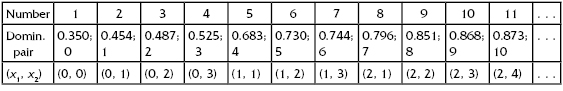
Let us enumerate corresponding pairs of this dominating sequence with the number x⁽¹⁾. Now we have a system consisting of two redundant groups: group 3 (data are on the lower lines of Table 5.5) and the newly composed group (data are in Table 5.7). On the basis of these data let us combine the final group for the considering system (Table 5.8 and Table 5.9).

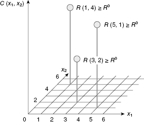
TABLE 5.8 Final Data for Solving the Optimal Redundancy Problems for the Illustrative Example

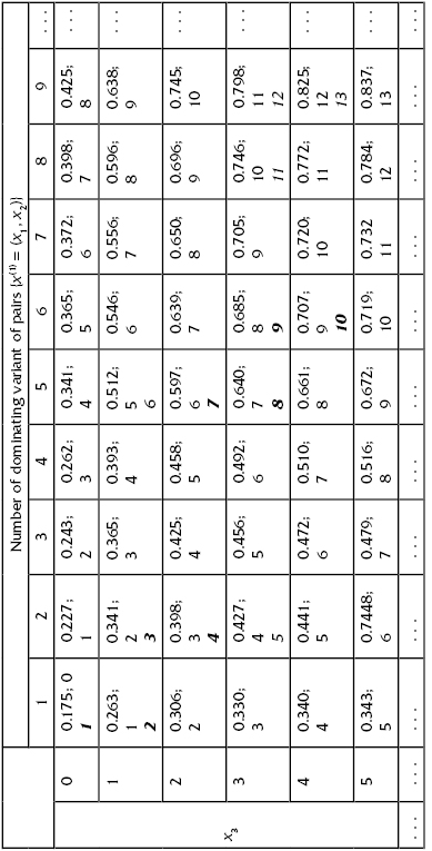
TABLE 5.9 Final Dominating Sequence for the System

5.2.3 Solving the Direct and Inverse Problems of Optimal Redundancy

Using Table 5.7, it is easy to get solutions for both direct and inverse problems of optimal redundancy (see Fig. 5.6). For instance, if one needs to find the best redundant unit allocation to satisfy the requirement R ≥ 0.8, then from Table 5.7 we find that the solution for corresponding value (R = 0.825) is in cell (x⁽¹⁾ = 9, x₃ = 4). The cost of redundant units in this case is 12. In turn, for x⁽¹⁾ = 9 one finds that this corresponds to x₂ = 1 and x₂ = 2.

FIGURE 5.6 Final dominating sequence for the system.

Thus, the solution of the inverse problem is (x₁ = 2, x₂ = 2, x₃ = 3).

If there is a limitation on the redundant units total cost equal to 10, then from Table 5.7 one finds that corresponding maximum value of probability of failure-free operation (PFFO) is 0.746. This solution corresponds to a cell (x⁽¹⁾ = 8, x₃ = 3). In turn, for x⁽¹⁾ = 8 one finds that this corresponds to x₁ = 1 and x₂ = 2.

Thus, the solution of the inverse problem is (x₁ = 1, x₂ = 2, x₃ = 3).

There are two ways of choosing redundant groups for composing a dominating sequence (see Fig. 5.7).

FIGURE 5.7 Two methods of choosing redundant groups for composing a dominating sequence.

For computer solution, both types are equivalent. However if one needs to make calculations by hand, then the dichotomous way gives a substantial decrease in calculations.

Chronological Bibliography

Bellman, R. 1957. Dynamic Programming. Princeton University Press.

Bellman, R., and Dreyfus, S. E. 1962. Applied Dynamic Programming. Princeton University Press.

Kettelle, J. D., Jr.Jr. 1962. “Least-coast allocation of reliability investment.” Operations Research, no. 2.

Li, J. 1966. “A bound dynamic programming for solving reliability redundancy optimization.” Microelectronics Reliability, no. 10.

Ushakov, I. A. 1969. Method of Solving Optimal Redundancy Problems under Constraints (in Russian). Sovetskoe Radio.

Misra, K. B. 1971. “Dynamic programming formulation of the redundancy allocation problem.” International Journal of Mathematical Education in Science and Technology, no. 3.

Yalaoui, A., Chatelet, E., and Chu, C. 2005. “A new dynamic programming method for reliability and redundancy allocation in a parallel-series system.” IEEE Transactions on Reliability, no. 2.