CHAPTER 3
Method of Lagrange Multipliers
One of the first attempts to solve the optimal redundancy problem was based on the classical Lagrange Multiplier Method. This method was invented and developed by great French mathematician Lagrange (see Box). This method allows one to get the extreme value of the function under some specified constraint on another involved function in the form of equality. The Lagrange Multiplier Method is applicable if both functions (optimizing and constraining) are monotone and differentiable.

Strictly speaking, this method is not appropriate for optimal redundancy problem solving because the system reliability and cost are described by functions of discrete arguments xi (numbers of redundant units) and the restrictions on accessible resources (or on required values of reliability) are fixed in the form of inequalities.
Nevertheless, this method is interesting in general and also gives us some useful hints for the appropriate solution of some practical problems of a discrete nature.
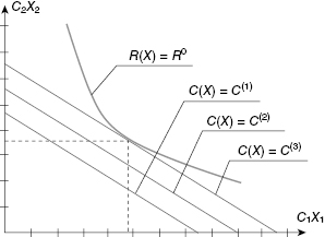
Let us begin with the direct optimal redundancy problem (Fig. 3.1 below). To solve this problem, we construct the Lagrange function, ![]() :
:
(3.1) ![]()
where C(X) and R(X) are the cost of the system redundant units and the system reliability, respectively, if there are X redundant units of all types, ![]()
Figure 3.1 Procedure of solving the direct problem of optimal redundancy.
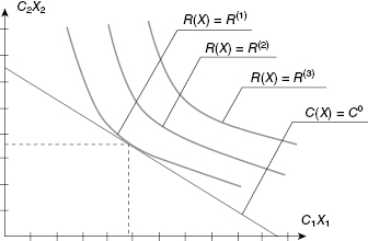
The goal is to minimize C(X) taking into account constraints in the form of R(Xopt) = R0. Thus, the system of equations to be solved is
(3.2) 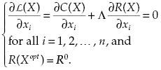
The values to be found are: ![]() , i = 1, 2, …, n, and Λ.
, i = 1, 2, …, n, and Λ.
If both function C(X) and R(X) are separable1 and differentiable, the first n equations of (3.2) can be rewritten as

On a physical level, Equation (3.3) means that for separable functions ![]() and C(X), the optimal solution corresponds to equality of relative increments of reliability of each redundant group for an equal and infinitesimally small resources investment.
and C(X), the optimal solution corresponds to equality of relative increments of reliability of each redundant group for an equal and infinitesimally small resources investment.
(3.4) 
In the general case, Equation (3.3) yields no closed form solution but it is possible to suggest an algorithm for numerical calculation:
(3.5) 
Of course, one would like to choose a value of
(3.6) 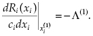
(3.7) ![]()
The stopping rule: X(N) is accepted as the solution if the following condition holds:
(3.8) ![]()
where ε is some specified admissible discrepancy in the final value of the objective function R(X).
Solution of the inverse optimal redundancy problem (Fig. 3.2) is analogous. The Lagrange function is:
(3.9) ![]()
and the equations are:

Figure 3.2 Procedure of solving the inverse problem of optimal redundancy.
The optimal solution has to be found with respect to goal function C(X). The stopping rule in this case is
(3.11) ![]()
where ε* is some specified admissible discrepancy in the final value of the goal function C(X).
Unfortunately, there is only one case where the direct optimal redundancy problem can be solved in a closed form. This is the case of a highly reliable system with active redundancy where:
(3.12) ![]()
or
(3.13) ![]()
that is, instead of maximizing R(X), one can minimize Q(X) and find the needed optimal solution.
Taking into account that both objective functions are separable, Equation (3.10) can be written as:
(3.14) 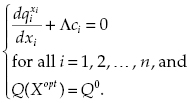
From equation
(3.15) 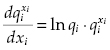
we can finally write

Now returning to the last equation in Equation (3.10), we have
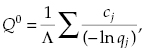
and, consequently, the Lagrange multiplier has the form
(3.18) 
From Equation (3.16), one has
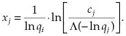
Finally, after substitution of Equation (3.17) into Equation (3.19), one gets
(3.20) 
Hardly anybody would be happy to deal with such a clumsy formula!
The solutions obtained by the Lagrange Multiplier Method are usually continued due to requirements to the objective functions. Immediate questions arise: Is it possible to use an integer extrapolation for each non-integer xi? If this extrapolation is possible, is the obtained solution optimal?
Unfortunately, even if one tries to “correct” non-integer solutions by substituting lower and upper integer limits ![]() , this very rarely leads to an optimal solution! Moreover, enumerating all 2n possible “corrections” can itself be a problem. We demonstrate this statement on a simple example.
, this very rarely leads to an optimal solution! Moreover, enumerating all 2n possible “corrections” can itself be a problem. We demonstrate this statement on a simple example.
Note
1 Taking the logarithm of multiplicative function R(X), one gets an additive function of logarithms of multipliers.
Chronological Bibliography
Everett, H. 1963. “Generalized Lagrange multiplier method for solving problems of optimum allocation of resources.” Operations Research, no. 3.
Greenberg, H. J. 1970. “An application of a Lagrangian penalty function to obtain optimal redundancy.” Technometrics, no. 3.
Hwang, C. L., Tillman, F. A., and Kuo, W. 1979. “Reliability optimization by generalized Lagrangian-function and reduced-gradient methods.” IEEE Transactions on Reliability, no. 28.
Kuo, W., Lin, H. H., Xu, Z., and Zhang, W. 1987. “Reliability optimization with the Lagrange-multiplier and branch-and-bound technique.” IEEE Transactions on Reliability, no. 5.