CHAPTER 11
Optimal Redundancy in Multistate Systems
Solving the problems of optimal redundancy allocation for multistate systems (MSS) consisting of multistate units is more laborious than solving analogous problems for systems that have only two states: normal operation and failure.
Today, this problem is investigated in detail. To begin with, the works of Gregory Levitin and Anatoly Lisnjanskij have to be mentioned (a complete list of their papers is presented in the Bibliography to the chapter).
To gain a clearer perspective of this type of problem, we begin with a simple numerical example. Consider a series system of two different multistate units, each of which is characterized by several levels of performance. Performance may be measured by various physical values. Effectiveness of such system operation depends on the levels of performance of Unit 1 and Unit 2. These units are characterized by the parameters presented in Table 11.1 and Table 11.2.
TABLE 11.1 Characterization of Unit 1
| Level of performance (W1) | Probability p1 | Cost of a single unit |
|---|---|---|
| 100% | p11 = Pr{W1 = 100%} = 0.9 | c1 = 1 |
| 70% | p12 = Pr{W1 = 100%} = 0.05 | |
| 40% | p13 = Pr{W1 = 100%} = 0.04 | |
| 0% | p14 = Pr{W1 = 100%} = 0.01 |
TABLE 11.2 Characterization of Unit 2
| Level of performance (W1) | Probability p2 | Cost of a single unit |
|---|---|---|
| 100% | p21 = Pr{W2 = 100%} = 0.8 | c2 = 2 |
| 80% | p22 = Pr{W2 = 80%} = 0.18 | |
| 20% | p23 = Pr{W2 = 20%} = 0.01 | |
| 0% | p24 = Pr{W2 = 0%} = 0.01 |
Assume that the performance effectiveness of each unit can be improved by using loaded redundancy. Let us suppose that at each moment of time, the performance effectiveness of a redundant group is equal to the level of performance of the best component of the redundant group. Thus, the behavior of Unit 1, consisting of the main component and single redundant element, can be depicted as shown in Figure 11.1. For Unit 2, the analogous process is presented in Figure 11.2.
FIGURE 11.1 A realization of stochastic behavior of Unit 1, consisting of two elements, main and redundant. The shadowed area denotes the behavior of Unit 1.

FIGURE 11.2 A realization of stochastic behavior of Unit 2, consisting of two elements, main and redundant. The shadowed area denotes the behavior of Unit 2.

Further, assume that the entire system (series connection of Unit 1 and Unit 2) is characterized by the worst level of effectiveness of its units at each moment of time. In Figure 11.3, one can see the system behavior for the case when both units consist of a single main element.
FIGURE 11.3 A realization of stochastic behavior of the entire system when both its units consist of a single main element. The shadowed area denotes the behavior of the system.

The problem is to find the optimal number of redundant elements in the series system described above:
Now consider the construction of a dominating sequence during the optimization process. In principle, one has to construct a table like Table 11.3 and choose members of the dominating sequence.
TABLE 11.3 Construction of Dominating Sequence
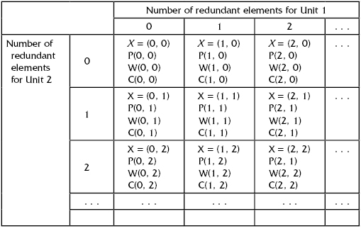
As one can see, in this case we deal with quadruplets of type:
{[Vector of numbers of redundant units];
[Discrete distribution of performance levels];
[Performance levels];
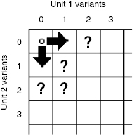
[System cost]}.The problem complicates due to necessity of calculations because “probabilities of performance levels” and “performance levels” are not numbers but vectors that need a special type of calculation. This aspect will be demonstrated shortly. Here we would like to note that there is no necessity to calculate quadruplets for all cells of Table 11.1. Fortunately, we can use Kettelle's Algorithm: members of dominating sequences are located around the table's diagonal and the corresponding cells form a simple connected area. It allows the use of the “dichotomy tree” procedure, that is, avoiding unnecessary calculations by cutting non-perspective branches (see Fig. 11.4). Indeed, consider bordering cells around the simple connected area (they are marked as “x”). There are no dominating cells in the area located in the upper right, and there are no dominating cells in the area located in the lower left.
FIGURE 11.4 Example of excluding non-perspective branches. Black arrows are members of dominating sequence; gray ones are trial tests that led to non-perspective variants marked by “x.” All cells marked with dark gray cannot contain dominating quadruplets.

Thus, in this case, the calculations occur to be sufficiently compact. However, as we mentioned above, some special calculations for each redundant group have to be done.
In accordance with the calculating procedure described above, one has to consider the first variant (0, 0), that is, just Unit 1 and Unit 2 with no redundancy at all, and find the quadruple. In this case, the resulting solution will be:
(11.1) 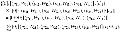
Here we use the following operators:
 , where, in turn,
 Of course, the same procedure can be presented in terms of U functions. One can write two “polynomials” of type
(11.2) 
Of course, the power of argument x has a very conditional sense: any value in “power” of vector has no common sense. To avoid such confusion, we will operate with sequences of triplets, quadruplets, and other “multiplets.”
Let us continue the numerical example because it helps us to not explain relatively simple procedures on an unnecessarily formal level. We now return to the series system, consisting of two units without redundancy. Numerical results are presented in Table 11.4.
TABLE 11.4 Initial State of the Process of Optimization

TABLE 11.5 Forehand Calculation of Performance Levels Distribution for Unit 1, Consisting of Two Elements, Main and Redundant

This leads to the following final result (see cells with the same background colors):
![]()
![]()
![]()
![]()
![]()
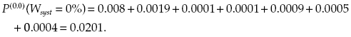
Cost of additional units in this case equals 0. As one can easily calculate, the average level of the system performance is equal to

Now let's make trial steps to the neighbor cells: check cells (1, 0) and (0, 1). Let us start with cell (1, 0) as it shown in Figure 11.4. First, find the distribution of performance levels for Unit 1 consisting of two elements, main and redundant.
On the basis of this table, one gets for Unit 1 the following distribution


![]()
Let us assume that the first step is made from (0, 0) to (1, 0) as is presented in Figure 11.5.
FIGURE 11.5 Direction of step 1 of the optimization process.

Using the results, presented above, one can compile Table 11.6, which gives performance levels distribution for the system characterized by vector of redundant elements X = (1, 0).
TABLE 11.6 Step 1 of the Optimization Process

This leads to the following final result:
![]()
![]()
![]()
![]()
![]()

Cost of additional units in this case equals 1. Average system's performance level equals

Then try another neighbor cell, namely (0, 1). Beforehand, one has to perform an additional calculation of performance levels distribution for Unit 2 consisting of two elements, main and redundant.
It is necessary to note that for parallel connection of multistate elements (that compiles a unit), one should realistically assume that the level of performance of the unit is equal to maximum among all currently operating elements. So, Table 11.7 represents results of calculation for Unit 2 that consists of two identical elements.
TABLE 11.7 Forehand Calculation of Performance Level Distribution for Unit 2, Consisting of Two Elements, Main and Redundant

On the basis of this table, one gets for Unit 2, consisting of two elements, the following distribution:


![]()
After such preparations, one can go to step 2 (see Fig. 11.6).
FIGURE 11.6 Direction of step 2 of the optimization process.
This step consists of construction of Table 11.8 and presents the system's performance levels distribution for the system configuration characterized by a vector of redundant elements X = (0, 1).
TABLE 11.8 Step 2 of the Process of Optimization

This leads to the following final result:
![]()
![]()
![]()
![]()
![]()
![]()
Cost of additional units in this case equals 2 units of cost. The average system's performance level equals

Thus, for vector (1, 0), one has additional cost equal to 1 and ![]() and for vector (0, 1) corresponding values equal to 2 and 0.671, so system configuration (1, 0) is dominating over configuration (0, 1), since a higher average performance level delivers with fewer expenses. It means that all vectors of type (0, k) are excluded from further analysis.
and for vector (0, 1) corresponding values equal to 2 and 0.671, so system configuration (1, 0) is dominating over configuration (0, 1), since a higher average performance level delivers with fewer expenses. It means that all vectors of type (0, k) are excluded from further analysis.
The next cells for which current trials have to be done are (1, 1) and (2, 0).
Avoiding simple but cumbersome calculations, let us present only the final results (see Table 11.9).
TABLE 11.9 Costs and Levels of Performance for Different Vectors of Redundant Elements
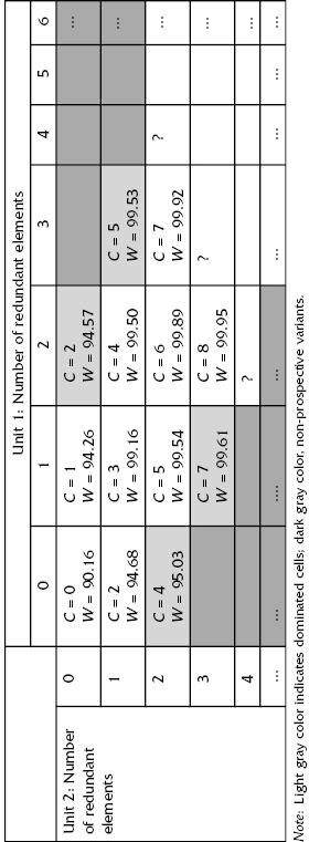
Table 11.9 is constructed as is shown in Figure 11.7. Table 11.9 probably needs some explanation. Vector (2, 0) is dominated by vector (0, 1), since vector (0, 1) is characterized by higher performance level for the same total cost of redundant units. So, all vectors of type (3, 0), (4, 0), …, (k, 0), … are excluded from further consideration. One observes the same type of domination for the following pairs: (3, 1) is dominated by (1, 2), vector (0, 2) is dominated by (1, 1), vector (1, 3) is dominated by (2, 2), and so on.
FIGURE 11.7 The process of step-by-step development of the optimization process.

Such trials and the selection of dominating vectors continued until the appearance of the first vector with the average level of performance higher than the required value of W0 for the direct problem of optimal redundancy, or until the total expense of all redundant elements does not exceed the given value C0 for the inverse problem. These comments become absolutely transparent if one takes a look at Figure 11.8.
FIGURE 11.8 Depiction of the process of compiling the dominating sequence.

From Table 11.9, one can see that the optimal solution for the requirement that the average level of system performance is not less than W0 = 0.999 is delivered by vector (3, 2), and the total expenses of redundant elements are 7 cost units. For the total expenses of redundant elements limited by C0 ≤ 5 cost units, one gets the maximum possible solution as vector (1, 2) that is characterized by W = 99.54%.
It is interesting to see what happens with the optimal solution if one changes the costs of elements. Let us assume that for the same system, cost of a single redundant element of the first type is c1 = 2 and the cost of an element of the second type c2 = 1.
In this case, optimal solutions found in Table 11.10 are: For the direct problem vector (2, 3), for which W = 99.95% and total expenses on redundant elements are equal to 7 cost units, and for the inverse problem the solution is (1, 3), for which W = 99.54% and total expenses are C = 5.
TABLE 11.10 Costs and Levels of Performance for Different Vectors of Redundant Elements for New Element's Costs

Solution of optimal redundancy problems for a system consisting of several multilevel units seems a bit cumbersome. However, let us note that all enumerative methods, like dynamic programming, are practically unsolvable without computerizing calculations. The numerical example above was solved with the help of simple programs using Microsoft Excel.
For complex systems consisting of n multiple multistate units, one can compile a simple program for a mainframe computer. The algorithm should include the following steps.
Such a solution appears a bit clumsy and laborious. However, the computer calculating program is relatively simple and the solution can be obtained easily enough; final results are presented in the form of a dominating sequence (in Kettelle's terminology), so the solutions for direct and/or inverse optimal redundancy problems can be easily found.
We restrict ourselves by consideration of this simple and more or less transparent illustrative example. In the last few years this problem has generated a number of interesting and theoretically deep publications, as the reader can see from the Bibliography. However, we think that more detailed consideration of this problem could lead us too far from the “highway” of main practical optimal redundancy tasks.
Chronological Bibliography
Reinschke, K. 1985. “Systems consisting of units with multiple states.” In Handbook: Reliability of Technical Systems, I. Ushakov, ed. Sovetskoe Radio.
El-Neweihi, E., Proschan, F., and Sethuraman, J. 1988. “Optimal allocation of multistate components.” In Handbook of Statistics, vol. 7: Quality Control and Reliability, P. R. Krishnaiah and C. R. Rao, eds. North-Holland.
Ushakov, I. 1988. “Reliability analysis of multi-state systems by means of modified generating function.” Elektronische Informationsverarbeitung und Kybernetik, no. 3.
Levitin, G., and Lisnianski, A. 1998. “Joint redundancy and maintenance optimization for multistate series-parallel systems.” Reliability Engineering and System Safety, no. 64,.
Levitin, G., Lisnianski, A., Ben Haim, H., and Elmakis, D. 1998. “Redundancy optimization for series-parallel multi-state systems.” IEEE Transactions on Reliability, no. 2.
Levitin, G., and Lisnianski, A. 1999. “Importance and sensitivity analysis of multi-state systems using universal generating functions method.” Reliability Engineering and System Safety, no. 65.
Levitin, G., and Lisnianski, A. 2000. “Optimal replacement scheduling in multi-state series-parallel systems.” Quality and Reliability Engineering International, no. 16.
Levitin, G., Lisnianski, A., and Ben Haim, H. 2000. “Structure optimization of multi-state system with time redundancy.” Reliability Engineering and System Safety, no. 67.
Levitin, G. 2001. “Redundancy optimization for multi-state system with fixed resource-requirements and unreliable sources.” IEEE Transactions on Reliability, no. 50.
Levitin, G., and Lisnianski, A. 2001. “A new approach to solving problems of multi-state system reliability optimization.” Quality and Reliability Engineering International, no. 47.
Levitin, G., and Lisnianski, A. 2001. “Structure optimization of multi-state system with two failure modes.” Reliability Engineering and System Safety, no. 72.
Levitin, G. 2002. “Optimal allocation of multi-state elements in linear consecutively-connected systems with delays.” International Journal of Reliability Quality and Safety Engineering, no. 9.
Levitin, G., Lisnianski, A., and Ushakov, I. 2002. “Multi-state system reliability: from theory to practice.” Proceedings of the 3rd Internationall Conference on Mathematical Models in Reliability, Trondheim, Norway.
Levitin, G. 2003. “Optimal allocation of multi-state elements in linear consecutively-connected systems.” IEEE Transactions on Reliability, no. 2.
Levitin, G. 2003. “Optimal multilevel protection in series-parallel systems.” Reliability Engineering and System Safety, no. 81.
Levitin, G., Dai, Y., Xie, M., and Poh, K. L. 2003. “Optimizing survivability of multi-state systems with multi-level protection by multi-processor genetic algorithm.” Reliability Engineering and System Safety, no. 82.
Levitin, G., Lisnianski, A., and Ushakov, I. 2003. “Reliability of multi-state systems: a historical overview.” Mathematical and Statistical Methods in Reliability, no. 7.
Lisnianski, A., and Levitin, G. 2003. Multi-State System Reliability: Assessment, Optimization and Applications. World Scientific.
Levitin, G. 2004. “A universal generating function approach for analysis of multi-state systems with dependent elements.” Reliability Engineering and System Safety, no. 3.
Nourelfath, M., and Dutuit, Y. 2004. “A combined approach to solve the redundancy optimization problem for multi-state systems under repair policies.” Reliability Engineering and System Safety, no. 3.
Ramirez-Marquez, J. E., and Coit, D. W. 2004. “A heuristic for solving the redundancy allocation problem for multi-state series-parallel systems.” Reliability Engineering and System Safety, no. 83.
Ding, Y., and Lisnianski, A. 2008. “Fuzzy universal generating functions for multi-state system reliability assessment.” Fuzzy Sets and Systems, no. 3.
Tian, Z, Zuo, M. J., and Huang, H. 2008. “Reliability-redundancy allocation for multi-state series-parallel systems.” IEEE Transactions on Reliability, no. 2.